The ribbon contains a Context tab for most objects. The Context tabs provides relevant options based on the selected object. Primary Context tabs include:
Model Context Tab

The Model Context tab becomes active when the Model object is selected in the Outline. The Model Context tab contains options for creating objects related to the model, as described below.
| Option | Description |
|---|---|
| Import Geometry/Reload | The import option for geometry is labeled Import Geometry if no primary geometry has been imported and Reload if a geometry has been imported. Therefore, the Reload option imports secondary geometries into your analysis. See the Geometry Imports description below. |
| Part Transform | Inserts a Geometry Transforms folder object that houses all of the part transformations (via Part Transform objects) that you create. |
| Create Table | Inserts a Table object plus a Tables folder that
houses all of the tables you create. This icon has two menu options:
See Using Tables for details. |
| Body Merge | Inserts a body merge object that combines multiple solid bodies into a single body. The selected bodies must share at least one face. See Body Merge for details. |
| Connections |
Becomes available only if a Connections object is not already included in the Outline (such as a model that is not an assembly), and you wish to create a connections object. See the Connections Context Tab topic below. Connection objects include contact regions, joints, and springs. You can transfer structural loads and heat flows across the contact boundaries and "connect" the various parts. See the Contact section for details. A joint typically serves as a junction where bodies are joined together. Joint types are characterized by their rotational and translational degrees of freedom as being fixed or free. See the Joints section for details. You can define a spring (longitudinal or torsional) to connect two bodies together or to connect a body to ground. See the Springs section for details. |
| Cross Sections | Inserts a desired cross section type. |
| Virtual Topology | You can use the Virtual Topology option to reduce the number of elements in a model by merging faces and lines. This is particularly helpful when small faces and lines are involved. The merging will affect meshing and selection for loads and supports. See Virtual Topology Context Tab below as well as the Virtual Topology Overview section for additional details. |
| Construction Geometry | See the Specifying Construction Geometry section for additional details. |
| Boundary Conditions | Define boundary conditions to be used across multiple analysis systems included in your simulation. See the Specifying Model-Level Boundary Conditions section for more information. |
| Condensed Geometry | Inserts a Condensed Geometry object. See the Condensed Geometry Context Tab topic below as well as the Substructure Analysis section for additional information. |
| Fracture | Inserts a Fracture object. See the Fracture Context Tab topic below as well as the Performing a Fracture Analysis section for additional information. |
| AM Process | Inserts an AM Process object. By default, it is inserted along with the child object Build Settings. You use this object when you are performing an additive manufacturing simulation. Also see the AM Process Context Tab topic below. |
| Measures | Inserts a Measures object. See the Measures Context Tab topic below. |
| Mesh Workflows | Inserts a Mesh Workflows object. Also, see the Mesh Workflows Context topic below. |
| Mesh Edit | Inserts a Mesh Edit object. Also see the Mesh Edit Context topic below. |
| Mesh Numbering | Enables you to renumber the node and element numbers of a generated meshed model consisting of flexible parts. See the Specifying Mesh Numbering section for details. |
| Solution Combination | Combines multiple environments and solutions to form a new solution. A solution combination folder can be used to linearly combine the results from an arbitrary number of load cases (environments). Note that the analysis environments must be static structural with no solution convergence. Results such as stress, elastic strain, displacement, contact, and fatigue may be requested. To add a load case to the solution combination folder, right-click the worksheet view of the solution combination folder, choose add, and then select the scale factor and the environment name. An environment may be added more than once and its effects will be cumulative. You may suppress the effect of a load case by using the check box in the worksheet view or by deleting it through a right-click. For more information, see Solution Combination. |
| Fatigue Combination | Inserts a Fatigue Combination object. When you are running an analysis that includes multiple systems that each include a Fatigue Tool object, the Fatigue Combination feature enables you to sum (generate a sum total of) the Damage results for all of the linked systems. This option only supports all analysis types that support the use of the Fatigue Tool. |
| Ply | When you select a ply object, the Ply group displays and
contains the Direction drop-down menu. The options of the menu
enable you to graphically display ply and element directions for imported ply structures.
|
Symmetry Context Tab
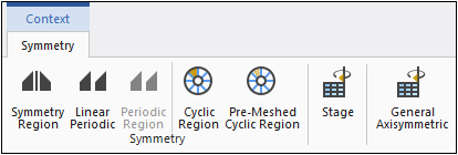
Based on your analysis type, the Symmetry Context tab includes options to insert Symmetry Region (including Linear Periodic), Periodic Region, Cyclic Region, Pre-Meshed Cyclic Region, Stage, and General Axisymmetric objects.
Connections Context Tab
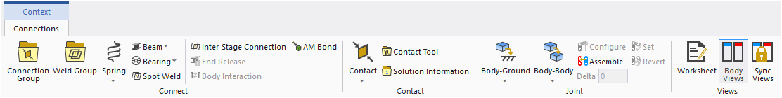
The Connections Context tab includes the following options and functions:
| Option | Description |
|---|---|
| Inserts a Connection Group object. | |
| Inserts a Spring object, either or | |
| Inserts a Beam object, either or . | |
| Inserts a Bearing object, either or . | |
| Inserts a Spot Weld object. | |
| Interstage | Inserts an Interstage object.. |
| Inserts an End Release object. | |
| See the Body Interactions in Explicit Dynamics Analyses section for additional information. | |
| AM Bond | Inserts an AM Bond object. |
| Inserts a specific type of Contact Region. | |
| Contact Tool | Inserts a Contact Tool object. |
| Solution Information | Insert a Solution Information object. |
| Enables you to insert and specify a certain type of Body-to-Ground Joint object. | |
| Enables you to insert and specify a certain type of Body-to-Body Joint object. | |
| , , and options and Delta field | Graphically configure the initial positioning of a joint. See the Example: Configuring Joints example. The
option performs the assembly of the model, finding the closest part configuration
that satisfies all the joints. Important: When a model contains a Point On Curve joint, the Configure and Assemble options are disabled for all the joints. This is also the case for a redundancy analysis that includes a Point On Curve joint. |
| Toggles the display of parts and connections in separate auxiliary windows for contact regions, beams, bearings, joints, and spring connections. | |
| When the option is selected, you can select this option synchronize the movements of your model in the Geometry window with the views of the auxiliary windows. and vice versa. |
Virtual Topology Context Tab
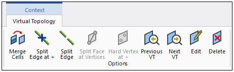
The Virtual Topology Context tab includes the following options:
| Option | Description |
|---|---|
| Creates Virtual Cell objects you can use to group faces or edges. | |
| and | Create Virtual Split Edge objects that enable you to split an edge to create two virtual edges. |
| Creates Virtual Split Face objects to split a face along two vertices to create 1 to N virtual faces. The selected vertices must be located on the face that you want to split. | |
| Creates Virtual Hard Vertex objects to define a hard point according to your cursor location on a face, and then use that hard point in a split face operation. | |
|
Previous VT/Next VT | Enable you to cycle through virtual topology entities in the sequence in which they were created. If any virtual topologies are deleted or merged, the sequence is adjusted automatically. See Cycling Through Virtual Entities in the Geometry Window. |
| Edits virtual topology entities. | |
| Deletes selected virtual topology entities, along with any dependents if applicable. |
Condensed Geometry Context Tab
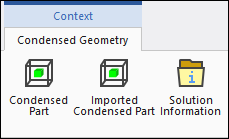
The Condensed Geometry Context tab enables you to apply the objects associated with substructuring, including the Condensed Part object, Imported Condensed Part, as well as a Solution Information object.
Fracture Context Tab
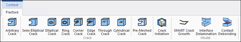
The Fracture Context tab enables you to insert the objects associated with a Fracture Analysis, including different Crack types, Crack Initiation, SMART Crack Growth, as well as progressive failure features in the form of Interface Delamination and Contact Debonding objects.
AM Process Context Tab
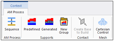
This tab displays when you insert an AM Process object into the Outline.
Measures Context Tab
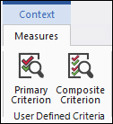
This tab displays when you insert a Measures object into the Outline. You use the this object to insert User Defined Criteria.
Mesh Workflows Context Tab
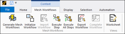
The Mesh Workflows Context tab helps you to:
Generate workflows from predefined steps that can be customized
Initialize, import, execute, and export the workflows
Visualize the workflow properties using the worksheet
The Mesh Workflows Context tab includes the following options:
| Option | Description |
|---|---|
| Generate Mesh Workflows | Generate mesh workflows. |
| Initialize Workflow | Initialize mesh workflow, transferring selected input geometry to the mesh workflow operations. Named Selections scoped to the input geometry translate into corresponding Labels after initializing the workflow. |
| Import Workflow | Import workflow steps from a .emx file. Import workflow is available after deleting steps and clearing data from the current workflow. |
| Execute Step | Initialize the workflow and execute the next step of the specified mesh workflow. |
| Execute All Steps | Initialize the workflow and execute all steps of the specified mesh workflow. |
| Export Workflows | Export the workflow steps as a template to a .emx file. |
| Complete Workflow | Complete the workflow by transferring generated data back to new mechanical geometry parts along with the corresponding part meshes. You cannot edit the specified mesh workflow type after completing the workflow. |
| Worksheet | Provides a view of the published mesh workflow operations, controls, and its properties. |
Mesh Edit Context Tab
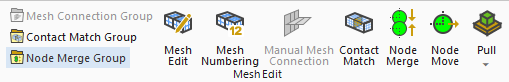
The Mesh Edit Context tab enables you to modify and create Mesh Connection objects that enable you to join the meshes of topologically disconnected surface bodies and also move individual nodes on the mesh. The Mesh edit Context tab includes the following options:
| Option | Description |
|---|---|
| Mesh Connection Group | Inserts a Mesh Connection Group folder object. |
| Manual Mesh Connection | Inserts a Mesh Connection Group folder that includes a Mesh Connection object. |
| Contact Match Group | Inserts a Contact Match Group folder object. |
| Contact Match | Inserts a Contact Match folder object. |
| Node Merge Group | Inserts a Node Merge Group folder object. |
| Node Merge | Selects geometries and merge coincident mesh nodes. |
| Node Move | Selects and move individual nodes on the mesh. Requires mesh generation. |
| Pull | Creates a mesh volume extrusion. |
| Body Views | Only visible when Mesh Connection object selected. Toggle button to display parts in separate auxiliary windows. |
| Sync Views | Only visible when Mesh Connection object selected. Toggle button that you can use when the Body Views button is engaged. Any change to the model in the Geometry window is reflected in both auxiliary windows. |
Geometry Imports
The options of the Geometry Imports Context tab will be determined by how you open Mechanical and whether you have imported geometry.
- Mechanical Opened Independently
The following Context tab displays when you open Mechanical independently, enabling you to open geometry or an external model file.
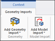
Both options include drop-down menus that provide a From File option to import files from a file location as well as a list of recently imported files that you can choose from.
- Mechanical Opened from Workbench
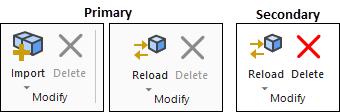
As illustrated, if you have not imported a geometry, the option Import Geometry enables you to do so. The Add Geometry Import option imports secondary geometries into your analysis. All options include drop-down menus that provide a From File option to import models from a file location as well as a list of recently imported geometries that you can choose from.
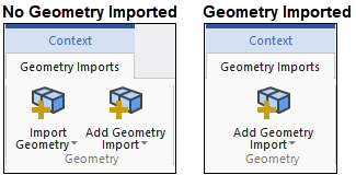
Similarly, when you select a child object (Geometry Import primary/secondary), the options of the primary object depend upon whether you have imported a geometry. For the secondary object, you use the Reload option to change your geometry. Or you can use the Delete option to remove the geometry from your analysis.
Geometry Context Tab
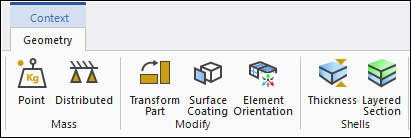
The Geometry context tab is active when you select the Geometry object in the Outline or any child objects (part/body) of the Geometry object. The tab includes the following options:
| Option | Description |
|---|---|
| Modify Geometry (not illustrated) | For electronic computer-aided design (ECAD) models, displays the ECAD Import pane. |
| Point | Specifies a . |
| Distributed | Specifies a Distributed Mass. |
| Transform Part | Becomes visible when you have a Part or Body selected. For the selected Part or Body, this option automatically scopes the geometry to a Part Transformation object. |
| Body Merge (not illustrated) | Becomes visible when you have a Part or Body selected. Combines the selected solid bodies into a single body. The bodies must share at least one face. See Body Merge for details. |
| Delete Part(s) (not illustrated) | Becomes visible when you have a Part or Body selected, enabling you to delete the selected part or body. Multiple part or body selection is supported. |
| Surface Coating | Specifies a . |
| Element Orientation | Specifies . |
| Imported Element Orientation | Available when you open Mechanical independently. Inserts an Imported Element Orientation folder object, an associated Element Orientation object, and displays the External Data dialog. Use this dialog to specify the desired external file(s) to import. |
| Thickness | For surface bodies, enables you to add a Thickness object. |
| Imported Thickness | Available when you open Mechanical independently. Inserts an Imported Thickness folder object, an associated Imported Thickness object, and displays the External Data dialog. Use this dialog to specify the desired external file(s) to import. |
| Layered Section | For surface bodies, enables you to add a object to define layers applied to surfaces. |
Imported Fields Context Tab
If the Geometry object includes an imported object, such as Imported Thickness or Imported Element Orientation, an Imported Fields Context menu displays when you select the imported object.
Materials Context Tab
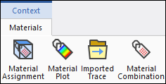
The Materials context tab is active when you select the Materials, Material Assignment, Material Plot, or Material Combination objects. Use this tab to employ the features related to the Materials object. Options include:
Imported Fields Context Tab
If you import Trace Mapping from an ECAD file, an Imported Trace group folder is placed under the Materials folder. This group folder displays the Imported Fields Context tab that includes the option Trace.
Imported Material Fields
If you import initial user-defined Field Variable values using the External Data system, an Imported Material Fields group folder is placed under the Materials folder.
As a result of your data import, the folder contains an Imported Material Field object. You can specify additional Imported Material Field objects using the option of this tab. In addition, the Variable Data tab displays when Imported Material Field objects are selected.
Tables Context Tab
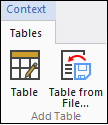
The Tables context tab is active when you select the Tables object. Use this tab to add tables for defining pressure, temperature, thermal condition, and convection loads. Options include:
Body Merge Context Tab
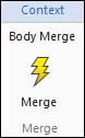
The Body Merge context tab is active when you select the Body Merge object. Click the Merge icon to execute a body merge.
Cross Section Context Tab
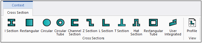
The Cross Section Context tab provides cross section type options that enable you to manually define a cross section for your line body model. There is also a Profile option that displays a window that enables you to view the cross section dimensions, during construction as well as when you are complete.
Coordinate Systems Context Tab
The Coordinate Systems Context tab is available when you have a user-defined Coordinate System object selected. It includes the following transformation options:
| Option | Description |
|---|---|
| Offset X/Y/Z | Create an Offset in the Transformations category of the Details view. These options require to enter a value. |
| Rotate X/Y/Z | Create a Rotate transformation in the Transformations category of the Details view. These options require to enter a value. |
| Flip X/Y/Z | Create a Flip transformation in the Transformations category of the Details view. These options flip the coordinate system about a desired axis. |
| Move Up/Move Down | Scroll up or down through the Transformations category properties/transformations that you have created. |
| Delete | Deletes a property/transformation from the Transformations category. |
Mesh Context Tab
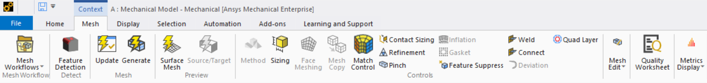
The Mesh Context Tab includes the following options:
In the Mesh Workflow group, the following option is available:
| Option | Description |
|---|---|
| Mesh Workflows | Generate Mesh Workflows based on predefined workflows that can be customized. |
In the Detect group, the following option is available:
| Option | Description |
|---|---|
| Feature Detection | Detects feature based on Feature Detection. |
In the Mesh group, the following options are available:
| Option | Description |
|---|---|
| Update | Updates a cell that references the current mesh. This includes mesh generation as well as generating any required outputs. |
| Generate | Generates a mesh. |
In the Preview group, the following options are available:
| Option | Description |
|---|---|
| Surface Mesh | Enables you to preview the Surface Mesh. |
| Source/Target | Enables you to preview the source and target meshes for scoped bodies. |
In the Controls group, the following options are available:
| Option | Description |
|---|---|
| Method | Selects Method Control. |
| Sizing | Selects Sizing Control. |
| Face Meshing | Selects Face Meshing Control. |
| Mapped Meshing | Selects Mapped Meshing Control. |
| Mesh Copy | Selects Mesh Copy Control. |
| Match Control | Selects Match Control. |
| Contact Sizing | Selects Contact Sizing Control. |
| Refinement | Selects Refinement Control. |
| Pinch | Selects Pinch Control. |
| Inflation | Selects Inflation Group. |
| Gasket | Selects Gasket Mesh Control. |
| Feature Suppress | Selects Feature Suppress Control. |
| Weld | Selects Weld Control. |
| Connect | Selects Connect Control. |
| Deviation | Selects Deviation Control. |
| Quad Layer | Selects Quad Layer Control. |
In the Mesh Edit group, the following options are available:
| Option | Description |
|---|---|
| Mesh Connection Group | Selects Mesh Connection Group. |
| Contact Match Group | Selects Contact Match Group. |
| Node Merge Group | Selects Node Merge Group. |
| Mesh Edit | Selects Mesh Edit. |
| Mesh Numbering | Selects Mesh Numbering. |
| Manual Mesh Connection | Creates manual Mesh Connections. |
| Contact Match | Selects Contact Match. |
| Node Merge | Selects geometries and merges coincident mesh nodes. |
| Node Move | Selects Node Move. |
| Pull | Creates a mesh volume extrusion. |
In the Quality Worksheet group, the following option is available:
| Option | Description |
|---|---|
| Quality Worksheet | Displays the Mesh Quality Worksheet. |
In the Metrics Display group, the following options are available:
| Option | Description |
|---|---|
|
Metric Graph |
Shows and/or hides the Mesh Metrics bar graph. |
|
Edges |
A drop-down menu options to change the display of your model, including:
These options are the same options that are available on the Meshing Edit Context Toolbar. |
|
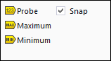
Probe, Max, and Min (Snap and Advanced) |
These are annotation display options. These options are not visible if the Mesh object Display Style property is set to the default setting, . Selecting the Max and/or Min buttons displays the maximum and minimum values for mesh criteria (Element Quality, Jacobian Ratio, etc.) that you have selected. The Probe feature is also criteria-based. You place a Probe on a point on the model to display an annotation on that point. Probe annotations show the mesh criterion-based value at the location of the cursor. See the Probe, Maximum, and Minimum topic below for more information. |
Environment Context Tab
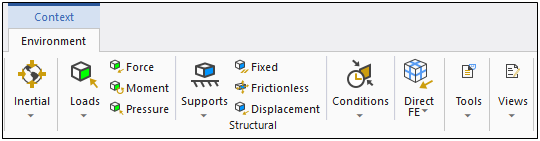
The Environment Context tab enables you to apply loads to your model. Tab groups and options vary depending on the type of analysis you are performing. For example, the groups and options for a Static Structural analysis is shown above.
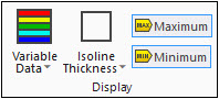
Environment Context Tab Display Group for Variable Data
When your analysis includes imported boundary conditions or imported thicknesses or you have specified spatial varying loads and displacements, the application displays contours or isoline representations of the associated variable data once you have generated the mesh on the model.
The Display group (shown below) becomes visible on the Environment Context Tab when variable data is available. The Variable Data drop-down menu provides the display options: , , and . When you select the display option, the Isoline Thickness drop-down menu enables you to change the thickness of the displayed lines. Options include (default), , or . The toolbar also contains options to display the Maximum and Minimum values of the imported data or spatial varying loading. You can toggle these min/max options on (default) and off.
Note:
The option is drawn based on nodal values. When drawing isolines for imported loads that store element values (Imported Body Force Density, Imported Convection, Imported Heat Generation, Imported Heat Flux, Imported Pressure, and Imported Surface Force Density), the program automatically calculates nodal values by averaging values of the elements to which a node is attached.
This feature is not available for Imported Loads that are scoped to nodal-based Named Selections.
If you select multiple Convection load objects that include variable data, the application displays only one solid color for the scoped entities.
Solution Context Tab
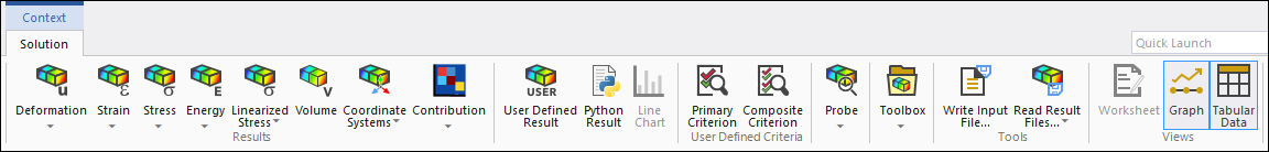
The Solution tab applies to Solution-level objects that either:
Never display contoured results (such as the Solution object), or
Have not yet been solved (no contours to display).
The options displayed on this tab are based on the type of analysis that is selected. The example shown above displays the solution options for a Static Structural analysis. Objects inserted using the Solution tab are automatically selected in the Outline.
The Applying Results Based on Geometry section outlines which bodies can be represented by the various choices available in the drop-down menus of the Solution tab.
Solution Information Tab
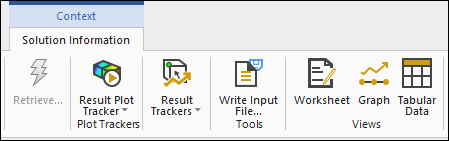
Selecting the Solution Information object displays a corresponding tab. The tab includes the option that you use to track background solution processes as well as the Result Tracker and Result Plot Tracker options. The Write Input File option as well as some additional display options, Worksheet, Graph, Tabular Data, are also included on the tab.
Result Context Tab
The Result tab provides display options for your solved result objects.
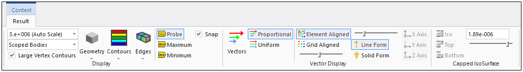
The following subsections describe the options available on this tab.
Scaling Menus for Deformed Shapes
The Display group contains the following scaling options for deformations.
Review the following topics for additional information:
Deformation Scale Menu
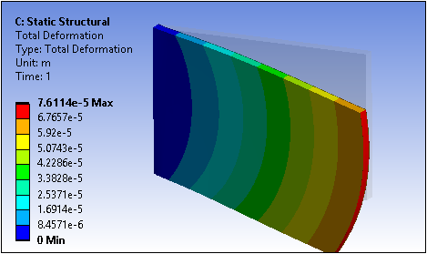
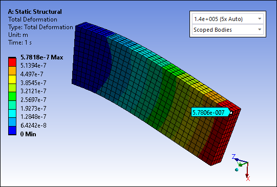
For results with an associated deformed shape, the scaling menu provides display selections.
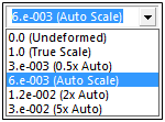
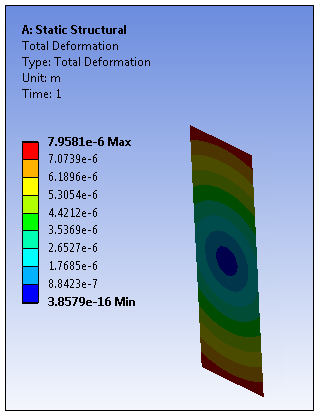
Scale factors precede the descriptions in parentheses in the list. The scale factors shown above apply to a particular model's deformation and are intended only as an example. Scale factors vary depending on the amount of deformation in the model. You can choose a preset option from the list, or you can enter a customized scale factor relative to the scale factors in the list.
For customized entries, the application follows a scheme where positive numbers affect the corresponding scaling differently than negative numbers. Positive numbers affect the factor (actual deformation) and negative numbers the factor (deformation is visible but not distorted). For example:
A scale factor of +2.0 equates to 2 times the True Scale factor
A scale factor of -2.0 equates to 2 times the Auto Scale factor
Available scale factors include:
Undeformeddoes not change the shape of the part or assembly.True Scaleis the actual scale.Auto Scalescales the deformation so that it's visible but not distorting.The remaining options provide a wide range of scaling.
The system maintains the selected option as a global setting like other options in the Result tab. As with other presentation settings, figures override the selection. For results that are not scaled, the menu selection has no effect.
Note: Most of the time, a scale factor selected by the application to create a deformed
shape that will show a visible deflection to allow you to better observe the nature of the
results. However, under certain conditions, the True Scale displaced
shape (scale factor = 1) is more appropriate and is therefore the default if any of the
following conditions are true:
Rigid bodies exist.
A user-defined spring exists in the model.
Large deflection is on.
This applies to all analyses except for Modal and Eigenvalue Buckling analyses (in
which case True Scale has no meaning).
Important:
- Scaling of Rigid Body Part Displacements in Modal or Eigenvalue Buckling Analyses
Note the following restrictions that apply when scaling rigid part displacements during Modal or Eigenvalue Buckling analyses.
(Currently) If you are performing a Modal or Eigenvalue Buckling analysis that includes rigid body parts, the application experiences a limitation while scaling and/or animating results.
The motion of rigid parts in Mechanical is characterized by the changes in the:
Position of the center of mass, referred to as linear displacement.
Euler angles of the element coordinate system, referred to as angular displacement.
Because of the difference in the nature of these concepts, a unified scaling algorithm that satisfies both scenarios has not yet been implemented for auto scaling. With the
Auto Scaleoption, Mechanical displays rigid parts as white asterisks at the centroid of the part. The application maintains the correct position of the rigid parts with respect to the flexible parts, however, the displayed asterisks do not indicate angular displacement or rotation.True Scalewill not properly display the shapes in Modal or Buckling analysis and should not be used.For the best scaling results when working on a Modal analysis (where displacements are not true), use the
Auto Scaleoption. If a given body's optimal scaling isTrueand another body's optimal scaling isAuto Scale, the graphical display of the motion of the bodies may not be optimal.
Important: For the following analyses and/or configuration conditions, Mechanical sets the scale factor to zero so that the image of the finite element model does not deform.
Random Vibration (PSD).
Response Spectrum.
Amplitude results for Harmonic Response analyses.
When the By property of a result is set to:
or
or
Relative Scaling
The menu provides the following "relative" scaling options. These options automatically scale deformations relative to preset criteria.
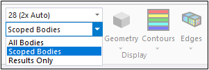
Display Menu
The Display drop-down menu enables you to view:
| Option | Description | Example |
|---|---|---|
| Regions of the model not being drawn as a contour are plotted as translucent even for unscoped bodies as long as the bodies are visible (not hidden) |
 | |
| Default setting. Regions of the model not being drawn as a contour are plotted as translucent for scoped bodies only. Unscoped bodies are not drawn. |
 | |
| Only the resultant contour or vector is displayed. |
 |
Limitations
Note the following limitations for the display selections:
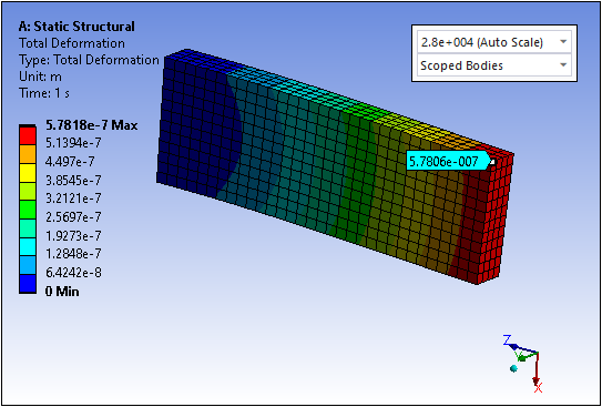
The and options support geometry-based scoping (Geometry Selection property = ) and Named Selections that are based on geometry selections or worksheet criteria.
The and options do not support Construction Geometry features Path and Surface.
The option does not support the Explicit Dynamics Solver.
For the Scoped Bodies option for results that are scoped across multiple entities (vertices, edges, faces, or volumes), all of these entities may not display because there are times when only the nodes of one of the shared entities are used in the calculation.
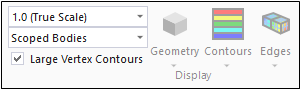
Large Vertex Contours
The Large Vertex Contours check box option is used for node-based result scoping. It toggles the size of the displayed dots that represent the results at the underlying mesh nodes on and off.
Geometry
You can observe different views from the Geometry drop-down menu, including:
| Option | Description |
|---|---|
| Displays the exterior results of the selected geometry. | |
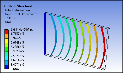
| For contour results, displays a collection of surfaces of equal value of the chosen result, between its minimum and a maximum as defined by the legend settings. The application displays the interior of the model only. | |
| Represents mainly a set of all points that equal a specified result value within the range of values for the result with additional features. This option provides three display selections. A display based on all points of a specified result, all points equal to and less than the specified result, and all points equal to and greater than the specified result value. Refer to Capped Isosurfaces section for a description of the controls with this option. This view displays contours on the interior and exterior. | |
| Displays planes cutting through the result geometry; only previously drawn Section Planes are visible. |
Contours
The Contours drop-down menu enables you to change the way you view your results. Options include:
| Option | Description |
|---|---|
| Displays gradual distinction of colors. | |
| Displays the distinct differentiation of colors. | |
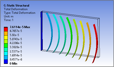
| Displays a line at the transition between values. | |
| Displays the model only with no contour markings. |
Edges
What is displayed by the options of the Edges drop-down menu, depends upon the selections you make in the other result display menus.
| Option | Description | ||||
|---|---|---|---|---|---|
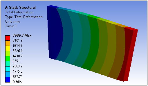
| Displays the result in its deformed state. The result's display is based on
your selections in the Geometry and
Contours menus (see above). Example
| |||||
|
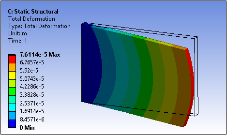
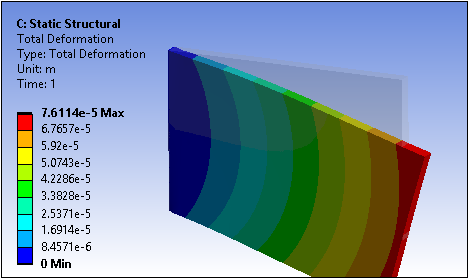
Displays the result with an undeformed wireframe overlay, as illustrated by the first image below. By default, this undeformed display is only supported for the option of the Geometry menu. The , , and options of the Geometry menu display the result with the wireframe overlay in a deformed state, as illustrated. Option: Wireframe Not Deformed with Result
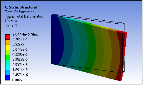
Option: Wireframe Deformed with Result
You can change this default setting for the deformation display using the preferences of the Options dialog. Under the Graphics category, set the Use Deformed Edge for Slice ISO Option to . For the , , and options, you can display the result in a deformed state and the wireframe overlay in an undeformed state, as illustrated below. Option: Wireframe Not Deformed with Result
Option: Wireframe Not Deformed with Result
| |||||
|
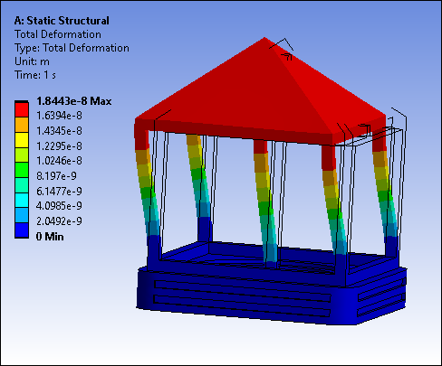
Displays the result with a translucent overlay of the undeformed model, as illustrated below. By default, this undeformed display is only supported for the Exterior option in the Geometry menu. The , , and options display the result with the translucent overlay of the model in a deformed state, as illustrated. Option - Translucent Overlay Not Deformed
Option - Translucent Overlay Deformed with Result
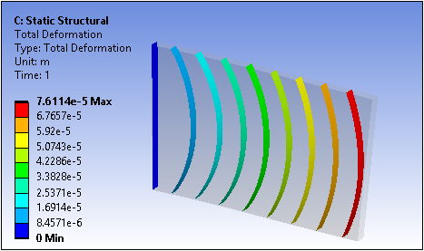
As stated above, you can change this default setting for the deformation display using the preferences of the Options dialog. Under the Graphics category, set the Use Deformed Edge for Slice ISO Option to . For the IsoSurface, Capped IsoSurface, and Section Planes options, you can display the result in a deformed state and the translucent overlay of the model in an undeformed state, as illustrated. Option: Translucent Overlay Not Deformed with Result
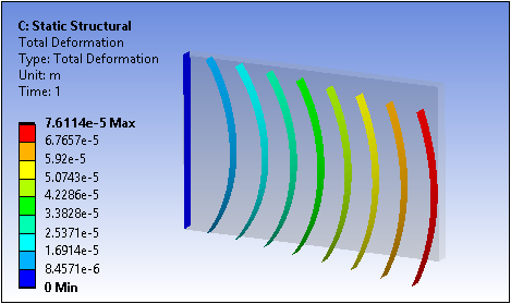
Option: Translucent Overlay Not Deformed with Result
| |||||
| Displays the result in its deformed state and includes mesh elements. The
result's display is based on your selections in the Geometry
and Contours menus. Example 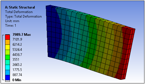 |

Probe, Maximum, and Minimum
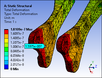
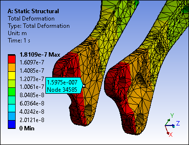
You use the Probe option to interactively place probe annotations on your model. If you display the Graphics Annotations window, you can view the result value at the location of your probe annotation, the unit of the result, as well as the coordinate values for the probe. You use the and options to display (or hide) annotations of the maximum and/or minimum values for the selected result.
Limitation: The and options consider only visible bodies. If you hide a body that includes one of these annotations, you could see a discrepancy between the minimum and maximum values displayed in the Details properties for the result versus the (new) location of the annotations.
The Snap option (active by default) automatically places probes on the nearest mesh node (the probe “snaps” to the node). For high order elements, this includes midside nodes as well as the centroids of element faces. Additionally, using the Show Mesh Entity ID in Snap-Probe Labels preference (also active by default) of the Graphics category in the Options dialog, the application automatically includes either the Node ID or the Element ID in the probe annotation label (see example below). Furthermore, the Graphics category (under the Interactive and Min/Max Probes category) includes a property, Show Detailed Information in Min/Max Probe Labels, that enables you to display additional information on the Min/Max probe, such as Node/Element ID and actual Min/Max values.
Tip: The application does not automatically save newly created probe annotations. You need to save the project manually.
Limitation: The Snap feature does not support the Geometry menu display options , , or .
| Probe Labelling | |
|
Probe Label
|
Probe Label with Node ID
|
Probe Display Font
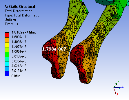
When the Probe option is selected and you move the cursor over your model, result values display. You can change the default display settings for the font using the Probe Tool and Hit Point Coordinate preference of the Graphics category in the Options dialog. This preference enables you to change the attributes (font, size, style, color) of the font displayed (illustrated below is Bold Calibri Size 18).
Probe Label and Scaling
Another Graphics category preference is the setting. This preference is the default setting. It enables the probe to be “flexible” and move with the deformed mesh whenever you make a change to the Deformation Scale Factor, as illustrated below. If turned off, the application deletes probe labels whenever you make a change to the scale factor.
Limitation: The application does not support the ability to flex a probe’s location using the Geometry menu display options , , or . If you place a probe when any of these options are active and then change the scaling, the application automatically removes/deletes the probe labels.
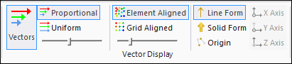
Vector Display
Using the Vector Display group, you can display results as vectors. This group includes various options for controlling the display of the vectors.
Note: These vector display options are also available for Element Orientations and certain vector based-loads.
When you select the Vectors option, the following associated options may be used.
| Option | Description |
|---|---|
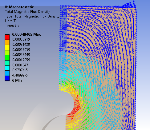
| Proportional | Displays vector length proportional to the magnitude of the result. |
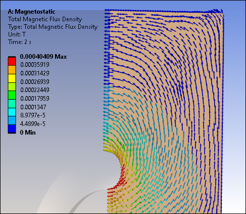
| Uniform | Displays a uniform vector length, useful for identifying vector paths. |
| Element Aligned | Displays all vectors, aligned with each element. |
| Grid Aligned | Displays vectors, aligned on an approximate grid. |
| Length Slider | Controls the relative length of the vectors in incremental steps from 1 to 10 (default = 5), as displayed in the tool tip when you drag the mouse cursor on the slider handle. |
| Grid Slider | Controls the relative size of the grid, which determines the quantity (density)
of the vectors. The control is in uniform steps from 0 [coarse] to 100 [fine]
(default = 20), as displayed in the tool tip when you drag the mouse cursor on the
slider handle. Note: This slider control is active only when the adjacent button is chosen for displaying vectors that are aligned with a grid. |
| Line Form | Displays vector arrows in line form. |
| Solid Form | Displays vector arrows in solid form. |
| Origin | Displays origin of the nodes included in the load and/or result. |
| X Axis/Y Axis/Z Axis | When solving principle stresses or principle strain, these buttons enable you to display (or hide) the vectors for Maximum Principal, Middle Principal, and Minimum Principal at each node. When solving Nodal Triads or Elemental Triads, these buttons enable you to display (or hide) the vectors for X Axis, Y Axis, and Z Axis at each node or element. |
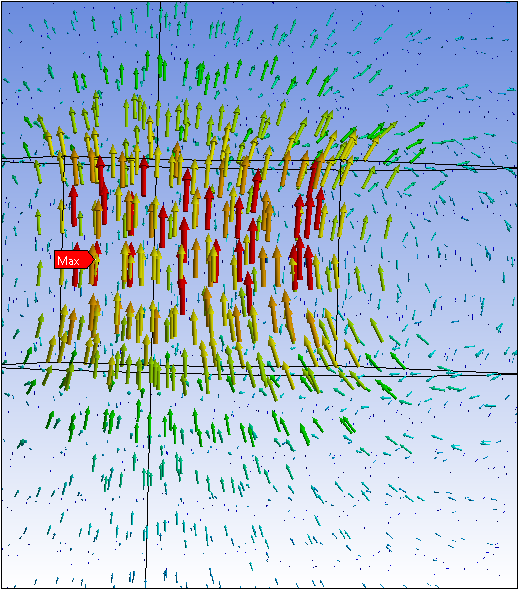
Vector Display Examples
Here are examples of uniform vectors identifying paths in line, solid, and origin form.
|
Line Form
|
Solid Form
|
Origin Form
|
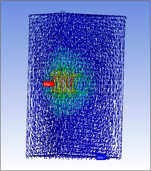
Here are vector arrows in solid form using the wireframe option.
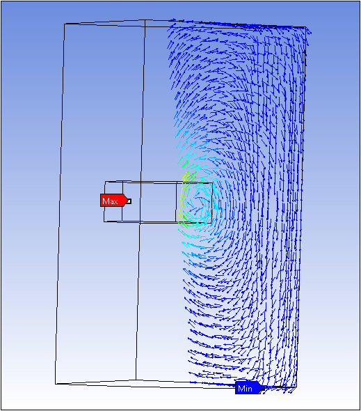
This is an example of uniform vector in solid form that have a Section Plane inserted.
Here is a zoomed-in example of uniform vectors with arrow scaling in solid form.