


The differences in the contact settings determine how the contacting bodies can move relative to one another. This category provides the following properties.
Type
Choosing the appropriate contact type depends on the type of problem you are trying to solve. If modeling the ability of bodies to separate or open slightly is important and/or obtaining the stresses very near a contact interface is important, consider using one of the nonlinear contact types (, , ), which can model gaps and more accurately model the true area of contact. However, using these contact types usually results in longer solution times and can have possible convergence problems due to the contact nonlinearity. If convergence problems arise or if determining the exact area of contact is critical, consider using a finer mesh (using the Sizing control) on the contact faces or edges.
The available contact types are listed below. Most of the types apply to Contact Regions made up of faces only.
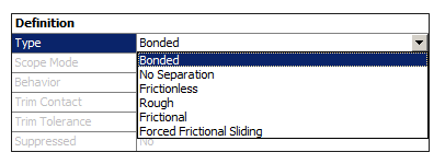
Bonded: This is the default configuration and applies to all contact regions (surfaces, solids, lines, faces, edges). If contact regions are bonded, then no sliding or separation between faces or edges is allowed. Think of the region as glued. This type of contact allows for a linear solution since the contact length/area will not change during the application of the load. If contact is determined on the mathematical model, any gaps will be closed and any initial penetration will be ignored. [Not supported for Rigid Dynamics. Fixed joint can be used instead.]
No Separation: This contact setting is similar to the Bonded case. It only applies to regions of faces (for 3D solids) or edges (for 2D plates). Separation of the geometries in contact is not allowed.
Frictionless: This setting models standard unilateral contact; that is, normal pressure equals zero if separation occurs. Therefore, gaps can form in the model between bodies depending on the loading. This solution is nonlinear because the area of contact may change as the load is applied. A zero coefficient of friction is assumed and allows free sliding. The model should be well constrained when using this contact setting. Weak springs are added to the assembly to help stabilize the model in order to achieve a reasonable solution.
Rough: Similar to the frictionless setting, this setting models perfectly rough frictional contact where there is no sliding. It only applies to regions of faces (for 3D solids) or edges (for 2D plates). By default, no automatic closing of gaps is performed. This case corresponds to an infinite friction coefficient between the contacting bodies. [Not supported for Explicit Dynamics analyses.]
Frictional: In this setting, the two contacting geometries can carry shear stresses up to a certain magnitude across their interface before they start sliding relative to each other. This state is known as "sticking." The model defines an equivalent shear stress at which sliding on the geometry begins as a fraction of the contact pressure. Once the shear stress is exceeded, the two geometries will slide relative to each other. The coefficient of friction can be any non-negative value. [Not supported for Rigid Dynamics. should be used instead.]
Forced Frictional Sliding: In this setting, a tangent resisting force is applied at each contact point. The tangent force is proportional to the normal contact force. This setting is similar to except that there is no "sticking" state. [Supported only for Rigid Dynamics]
By default the friction is not applied during collision. Collisions are treated as if the contact is frictionless regardless the friction coefficient. The following commands override this behavior and include friction in shock resolution (see Rigid Dynamics Command Objects Library in the Mechanical User's Guide for more information).
options=CS_SolverOptions()options.FrictionForShock=1Note that shock resolution assumes permanent sliding during shock, which may lead to unrealistic results when the friction coefficient is greater than 0.5.
Friction Coefficient: Enables you to enter a friction coefficient. Displayed only for frictional contact applications.
Note:
For the Bonded and contact Type, you can simulate the separation of a Contact Region as it reaches some predefined opening criteria using the Contact Debonding feature.
Refer to KEYOPT(12) in the Mechanical APDL Contact Technology Guide for more information about modelling different contact surface behaviors.
Scope Mode
This is a read-only property that displays how the selected Contact Region was generated. Either automatically generated by the application (Automatic) or constructed or modified by the user (Manual). Note that this property is not supported for Rigid Body Dynamics analyses.
Behavior
This property will appear only for 3D Face/Face or 2D Edge/Edge contacts. For 3D Edge/Edge or Face/Edge contacts, internally the program will set the contact behavior to Asymmetric (see below). Note that this property is not supported for Rigid Body Dynamics analyses.
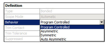
Sets contact pair to one of the following:
Program Controlled (Default for the Mechanical APDL solver): internally the contact behavior is set to the following options based on the stated condition:
Auto Asymmetric (see below): for Flexible-Flexible bodies.
Asymmetric (see below): for Flexible-Rigid bodies.
Symmetric (see below): for Flexible-Flexible bodies that are scoped to a Nonlinear Adaptive Region.
For Rigid-Rigid contacts, the Behavior property is under-defined for the Program Controlled setting. The validation check is performed at the Contact object level when all environment branches are using the Mechanical APDL solver. If the solver target for one of the environments is other than Mechanical APDL, then this validation check will be carried out at the environment level; the environment branch will become under-defined.
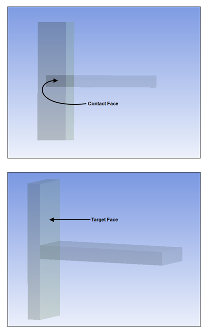
Asymmetric: Contact will be asymmetric for the solve. All face/edge and edge/edge contacts will be asymmetric. [In Explicit Dynamics analyses this is supported for Bonded connections.]
Asymmetric contact has one face as Contact and one face as Target (as defined under Scope settings), creating a single contact pair. This is sometimes called "one-pass contact," and is usually the most efficient way to model face-to-face contact for solid bodies.
The Behavior property setting must be if the scoping includes a body specified with rigid Stiffness Behavior.
Symmetric: Contact will be symmetric for the solve. The symmetric pairs will have the same contact characteristics (using KEYOPT(8)=1) except when the Nonlinear Adaptive Region object is present.
Auto Asymmetric: Automatically creates an asymmetric contact pair, if possible. This can significantly improve performance in some instances. When you choose this setting, during the solution phase the solver will automatically choose the more appropriate contact face designation. You can also designate the roles of each face in the contact pair manually. [In Explicit Dynamics analyses this option is available for Bonded connections; see Bonded Type.]
Note: Refer to KEYOPT(8) in the Mechanical APDL Contact Technology Guide for more information about asymmetric and symmetric contact selection.
Trim Contact
The Trim Contact feature can speed up the solution time by reducing the number of contact elements sent to the solver for consideration. For a Contact Region interface of a Condensed Part, this property enables you to reduce the number of master DOFs the application sends to the solver. Note that this feature is not supported for Rigid Body Dynamics analyses.
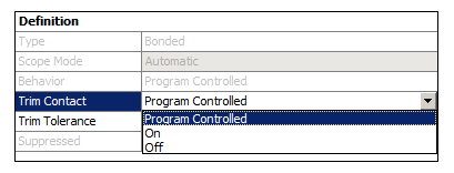
Trim Contact options include:
Program Controlled: This is the default setting. The application chooses the appropriate setting. Typically, the application sets Trim Contact to . However, if there are manually created contact conditions, no trimming is performed. By default, for Condensed Part generation, no trimming of the master DOFs is performed.
: During the process of creating the solver input file, checking is performed to determine the proximity between source and target elements. Elements from the source and target sides which are not in close proximity (determined by a tolerance) are not written to the file and therefore ignored in the analysis.
: No contact trimming is performed.
The checking process is performed to identify if there is overlap between the bounding boxes of the elements involved. If the bounding box of an element does not overlap the bounding box of an opposing face or element set, that element is excluded from the solution. Before the elements are checked, the bounding boxes are expanded using the Trim Tolerance property (explained below) so that overlapping can be detected.
Trim Tolerance
This property provides the ability to define the tolerance value that is used to expand the bounding boxes of the elements before the trimming process is performed.
This property is available for both automatic and manual contacts when the Trim Contact is set to . It is only available for automatic contacts when the Trim Contact is set to since no trimming is performed for manual contacts. For automatic contacts, this property displays the value that was used for contact detection and it is a read-only field. For manual contacts, enter a value greater than zero.
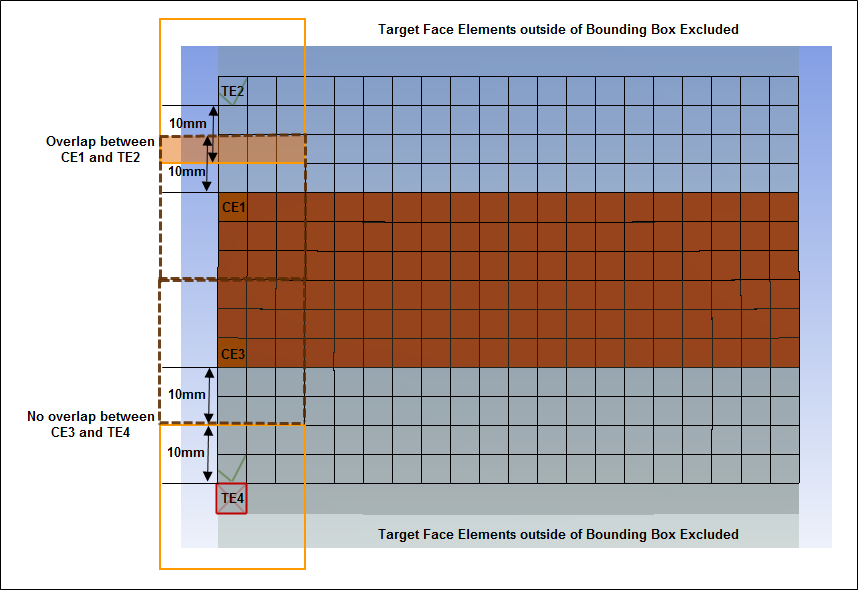
Note that a doubling expansion effect can result from the bounding box expansion since the bounding box of both the source and target elements are expanded. An example of the double expansion effect is illustrated below where the Trim Tolerance is defined as 10 mm. For simplicity sake, the size of the elements is specified as 5mm. Therefore, the bounding boxes for the contact/target elements will extend 10mm (two elements) in each direction as represented by the orange boxes, solid and dashed. For each face, Contact and Target, the number of elements that will be used are illustrated.
The brown area illustrated below represents the elements from the contact face. On the corresponding target side exist potential elements from the entire target face. The elements of the target face that will be kept are drawn in black. On the target Face, each element bounding box is expanded by 10mm and an overlap is sought against each element from the contact side. Referring to the image below, the bounding boxes between Contact Element 1 (CE1) and Target Element 2 (TE2) overlap and therefore TE2 is included in the analysis. Meanwhile, CE3 and TE4 do not overlap and as a result, TE4 is not included in the analysis. This results in a reduced number of elements in the analysis and, typically, a faster solution.
Contact/Target APDL Name
These properties are optional and only available for the Mechanical APDL solver. They enable you to specify an APDL parameter name for the contact and the target element types. Using these names, you can easily identify the contact and target element type and their corresponding real constant set that you can reference and use in a Commands (APDL) object.
Recommendation: Because element key options for all contact and target element types can be modified or set using the KEYOPT command with the ITYPE argument set CONT or TARG, Ansys recommends that you do not specify the Contact/Target APDL Name property using a variable that begins with "Cont" or "Targ," such as "Contact_1" or "Target _1."
If the Contact/Target APDL Name entry modifies an element key option (KEYOPT), the application will automatically modify all contact and target element types.
Suppressed
Specifies whether or not the Contact Region is included in the solution.