


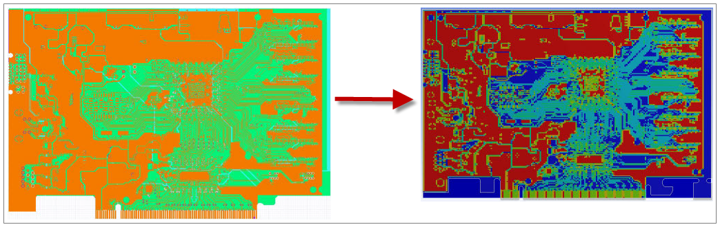
Mechanical's trace mapping feature provides a fast and efficient method to model Printed Circuit Boards (PCBs) and packages that would otherwise require an inordinate amount of time to process a geometry and mesh. Typically, the geometry that you produce in your electronic computer-aided design (ECAD) system contains a large number of bodies and therefore large amounts of data. Given the complexity of the system, producing a mesh can be very difficult. The trace mapping feature simplifies your model by modeling the geometry as dielectric layers and includes the effect of traces by mapping the metal fraction onto the dielectric layers.
Mapping takes place in two stages. As illustrated below, during the first stage, a representation of the layout is built upon a rectangular grid using the data from a specified ECAD layout. The cell size of the grid is governed by the smallest features in the layout that have to be resolved. This size can be controlled by the user and should be specified based on the resolution required. A metal fraction value is assigned to each cell depending on the contribution of metal to that cell. The metal fraction value ranges from 0 to 1, where the 0 value represents a pure dielectric material and 1 a pure metal material.
The conduction paths that connect the metal traces between the different layers, that is, the vias, can be specified as either hollow or solid (default).
|
Building a Representation Upon a Rectangular Grid | |
|
|
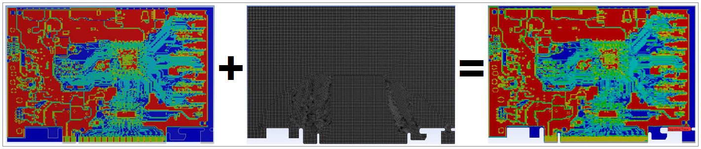
During the second stage, the metal fraction values are mapped from the source grid to the target mesh. Once the mesh is created, Mechanical then generates the mapped metal fractions. The sequence of this construction is illustrated below.
|
Mapping Metal Fractions | ||
|
|
General Workflow from Workbench
The following workflow describes the general steps to perform an analysis of a Printed Circuit Board that includes trace mapping.
Import supported ECAD files into External Data and update your project.
Add the supported Mechanical system to the project.
Add appropriate materials using Engineering Data.
You can open an ECAD layout geometry in an analysis system in Workbench once you have the proper file format. You can use SpaceClaim or SCDM.
Note: You can open Ansys EDB, ODB++, and IPC2581 files in Mechanical using the Geometry cell of the analysis system. An External Data system is not required until you import the trace mapping. See the ECAD Import section for more information.
Connect the Setup cell of the External Data system to the analysis system's Model cell.
Launch Mechanical. See the next section Trace Mapping for the specifics of setting up the Imported Trace object.
Specify vias as required.
Assign Dielectric material to the bodies. As needed, modify additional Geometry object properties.
Note: Reference temperatures specified on bodies are included in the solution calculation for any trace material contained in an element on the associated body.
Assign appropriate ECAD File to Imported Trace object.
Verify that the trace layout source is properly aligned with geometry.
Assign Metal material to imported trace layers.
Define and generate mesh.
Set discretization.
Generate the trace mapping.
Define boundary conditions.
Solve the analysis.
General Workflow from Mechanical
The following workflow describes the general steps to perform an analysis of a Printed Circuit Board that includes trace mapping.
Open the application from the Start Menu option Ansys 2024 R1 and select .
Insert an analysis system.
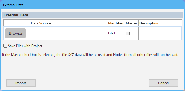
From the Materials object, select the Imported Trace option. The application automatically inserts the Imported Trace object into the tree and the External Data dialog displays. You use this dialog to specify the desired external file(s) you wish to import.
Note: If you have already selected a file and displayed the dialog, there are two additional context (right-click) menu options: and . The option re-opens the External Data dialog enabling you to modify the imported object's details and the option reloads data from the source file(s).
Select the Browse button. The following dialog displays.
Select a desired file using the File Name option.
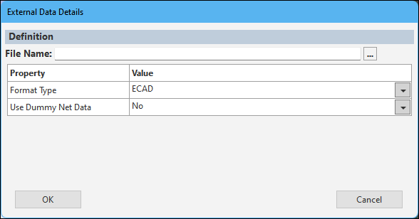
Specify a desired File Format and associated properties. Options include:
ECAD: Supported data files include ANSOFT ANF, ODB++ TGZ, IPC-2581 XML, or EDB DEF. The Use Dummy Net Data property specifies whether to import trace data belonging to the dummy net of the file.
ICEPAK: This format type supports ICEPAK BOOL or ICEPAK COND data.
Select the OK button and then the Import button. The data file is now associated with the object.
See the next section Trace Mapping for the specifics of setting up the Imported Trace object.
Specify vias as required.
Assign Dielectric material to the bodies. As needed, modify additional Geometry object properties.
Note: Reference temperatures specified on bodies are included in the solution calculation for any trace material contained in an element on the associated body.
Assign appropriate ECAD File to Imported Trace object.
Verify that the trace layout source is properly aligned with geometry.
Assign Metal material to imported trace layers.
Define and generate mesh.
Set discretization.
Generate the trace mapping.
Define boundary conditions.
Solve the analysis.
Requirements
This workflow requires the following components or systems:
Engineering Data: This component enables you to define materials required for the analysis. The materials defined the in the Engineering Data component will be available in the corresponding Mechanical model. For your convenience two materials (FR-4 and Copper Alloy) which commonly represent dielectric and metal in a PCB are available in the General Materials sample library.
Geometry: This component enables you to create or import the geometry representing the board or the package layout. The SpaceClaim geometry editor enables you to directly import the supported ECAD formats (see below) and automatically create a (trace layout) Geometry. See the ECAD section in Importing and exporting in the SpaceClaim documentation for details.
External Data: This component enables you to specify the ECAD file for import in Mechanical. The following ECAD File formats are supported for Trace Analysis:
- In Mechanical
Ansys EDB
ODB++
IPC2581
- In External Data
Ansoft ANF (External Data)
ODB++ TGZ
Icepak BOOL+INFO
Limitation: For this file type, when you are using the Linux platform, the metal fraction calculation is not supported when you start Workbench using remote access software.
Icepak COND+INFO
Once an ECAD file is specified in External Data, additional Rigid Transformation controls are available in the component to align the trace data with the geometry.
Important: If you are using release in 2024 R1 AFNIC Special Version, or a more current release, and you are opening a database/project created prior to release 2022 R1, the application may not successfully import trace data from ODB++, ANF, or BOOL+INFO files, if you 1) clear the data of the existing Imported Trace object and 2) attempt to reimport the upstream data.
To resolve the issue, right-click the Setup cell of the upstream External Data system that includes the trace files and select . Right-click again and select . Then select the context (right-click) menu option on the downstream system(s).
Mechanical Systems: The supported Mechanical systems enable you to import Trace Data, setup the analysis and solve. The following analysis are supported:
- Supported Structural Analysis Systems
Harmonic Response
LS-DYNA
LS-DYNA Restart
Modal
Static Structural
Transient Structural
- Supported Thermal Analysis Systems (Solid Bodies Only)
Steady-State Thermal
Transient Thermal
See Trace Mapping for the specifics of setting up an analysis.