


You can track, monitor, or diagnose problems that arise during any solution as well as view certain finite element aspects of the engineering model, using a Solution Information object, which is inserted automatically under a Solution object of a new environment or an environment included in a database from a previous release. You can also manually insert a Solution Information object under a Connections object for solver feedback.
This section examines the following uses of the feature:
Specifying Solution Information Properties
When you select a Solution Information object in the Outline, the following properties are available in the Details pane under the Solution Information category:
- Solution Output
The Solution Output property defines how you want solution response results to display. All of the options, described below, display results in real time as the solution progresses.
Important: The Solution Output property is not applicable to the Connections object.
(default): Displays the solution output file (in text format) from the appropriate solver (Mechanical APDL, Explicit Dynamics, etc.). This option is valuable to users who are accustomed to reviewing this type of output for diagnostics on the execution of their solver of choice. During the solution process, the default behavior of the solver output display is to scroll to the bottom of the log. However, if you scroll the log to another position, then the application maintains that view position. You resume automatic scrolling by pressing the End key.
Note: The text contents may be incomplete for a distributed solution involving Harmonic analyses or analyses featuring Cyclic Symmetry. See the DDOPTION command for additional information.
Solution Statistics: This option is supported for all Mechanical analysis systems using Mechanical APDL solver and for LS-DYNA analysis systems. It becomes available in the property drop-down list once you have completed your solution. Selecting this option displays the Worksheet. The Worksheet displays statistical information about your completed solution process as well as recommendations about how to improve the process. Using this information, you can make decisions to improve your solution time and performance. For example, you may decide to use a different solver or to change the number of cores being employed.
: This option is supported for all Mechanical analysis systems using Mechanical APDL solver. When selected, the option displays the Worksheet that contains two tabs to review information the solutions performed and about the evaluated results: Solution Tracking and Result Tracking. The Solution Tracking tab tracks information such as time to solve as well as the number of nodes and elements for each solution. The Result Tracking tab tracks a result's minimum and maximum values for each solution. Most common result types are supported for this feature, such as Total Deformation, stress, strain, etc.
Each tab presents a chart that graphs the data based on the data columns you select in the table. Each table heading provides a filter as well as a checkbox. Only two check boxes can be selected at one time. You can change chart display settings (lines or columns) as well as the labeling by right-clicking in the chart. In addition, you can right-click on a row and select the Delete option.
Note: You can change the default settings for the number of the solutions to be tracked using the Maximum Solutions to Store property and turn result tracking off using the Track Results property in the Analysis Settings and Solution of the Options dialog.
Resource Prediction: This option is available for Static Structural and stand-alone Modal analyses and displays resource prediction information in the Worksheet. Information includes time and memory predictions for the requested number of cores, charts of time and memory allocations for different core settings (maximum of 32), and suggestions, if applicable, such as whether an alternative solver type setting (structural only) improves resource allocations or whether there is insufficient memory.
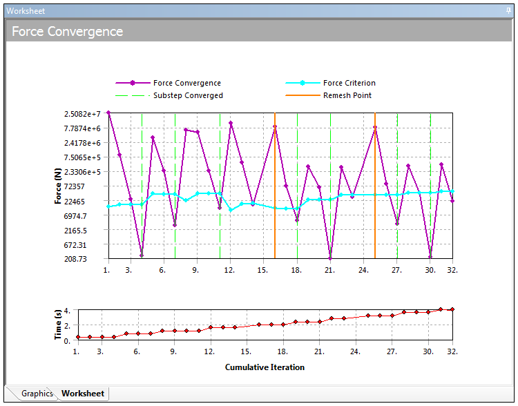
Choosing any of the following options for the Solution Output property displays a graph of that option as a function of Cumulative Iteration/Cycle (availability depends on the solver).
(Modal analysis only): This option displays the Worksheet with the label Participation Factor Summary.
Complex eigenvalues are available when the Damping property is set to Yes (except when the Solver Type is selected and the Store Complex Solution property is set to ). When the Damping property is set to No, only the Solver Type provides complex Eigenvalues.
When you have a complex eigenvalue solution, the Participation Factor Summary Worksheet displays Mode, Frequency, X Direction (Real), Y Direction (Real), Z Direction (Real), X Direction (Imaginary), Y Direction (Imaginary) and Z Direction (Imaginary). Otherwise the worksheet tables display Mode, Frequency, X Direction, Y Direction, Z Direction, Rotation X, Rotation Y and Rotation Z.
When you select option, the property Summary Type also displays and its options include:
(default): All tables are displayed in the Worksheet, including Participation Factor, Effective Mass, Cumulative Effective Mass Fraction, and Ratio of Effective Mass to Total Mass.
: Only the Participation Factor table is displayed in the worksheet.
: Only the Effective Mass table is displayed in the worksheet.
: Only the Cumulative Effective Mass Fraction table is displayed in the worksheet.
Ratio of Effective Mass to Total Mass: Only the Ratio of Effective Mass to Total Mass table is displayed in the worksheet.
Important: The unit system for all of the data displayed in the Participation Factor Summary Worksheet is the unit system for the Solver Unit System property in the Analysis Data Management category of the Analysis Settings object.
Note:The output option is not available when Cyclic Symmetry is active.
If the Campbell Diagram property is set to in the Modal system's Analysis Settings (multi-step Modal analysis), the Participation Factor Summary reported in the Worksheet is for the last rotational velocity/load step.
(Quasi-Static Solution only)
(Quasi-Static Solution only)
1 (magnetic current segments)
: Shows plots of total energy, reference energy, work done, and energy error.
: Shows plots of X, Y and Z momentum and X, Y and Z impulse for the model.
: Shows plots of internal energy, kinetic energy, hourglass energy and contact energy.
: displays the output of a Post Command snippet.
: This option displays the solution output (in text format) from the Topology Optimizer solver.
Mechanical also provides the following convergence charts for the Structural Optimization analysis. These options provide plots (in the Worksheet) for convergence values determined during the solution. This is useful for determining if the simulation is nearing convergence. All of these options have a plot for the combined objective value versus the Convergence Accuracy as defined in the Definition Analysis Settings for the Topology Optimization environment. Note that individual objective values can occur separately in a multi-step analysis. These options also include a plot for the convergence of the Response Constraint that you wish to observe (Mass, Volume, etc.).
: This option is the default option for a Structural Optimization analysis. This property plots the Mass Response Convergence against the criterion you specify in the Percent to Retain property of the Mass Constraint object (Response Constraint). The convergence chart will plot convergence against Percent To Retain (Min) and Percent To Retain (Max) criterion, if the constraint is defined by Range.
: This property plots the Volume Response Convergence against the criterion you specify in the Percent to Retain property of the Volume Constraint object (Response Constraint). The convergence chart will plot convergence against Percent To Retain (Min) and Percent To Retain (Max) criterion, if the constraint is defined by Range.
(Static Structural analyses only): Plots the stress response convergence against the criterion specified in the Maximum property of the Global Von-Mises Stress Constraint object. For multi-step analyses, the application provides fields to enable you to choose which Step Number corresponds to the stress constraint you wish to observe.
(Static Structural analyses only): Plots the local stress response convergence against the criterion specified in the Maximum property of the Local Von-Mises Stress Constraint object. For multi-step analyses, the application provides fields to enable you to choose which Step Number corresponds to the stress constraint you wish to observe.
(Static Structural analyses only): Plots the displacement response convergence against the criterion specified in X Component (Max)/Y Component (Max)/Z Component (Max) of the Displacement Constraint object. For multi-step analyses, the application provides fields to enable you to choose which Step Number corresponds to the displacement constraint you wish to observe.
(Static Structural analyses only): Plots the reaction force response convergence against the criterion specified in X Component (Max)/Y Component (Max)/Z Component (Max) of the Reaction Force Constraint object. For multi-step analyses, the application provides fields to enable you to choose which Step Number corresponds to the reaction force constraint you wish to observe.
(applicable for Modal analyses): Plots the Natural Frequency Response convergence against the criterion specified in the Minimum Frequency and Maximum Frequency properties of the Natural Frequency Constraint object (Response Constraint). The application provides a field to enable you to specify a Mode Number corresponding to a natural frequency range you wish to observe.
(applicable when criterion is entered for the Maximum property of the Manufacturing Constraint object): Plots the manufacturing response convergence against the criterion specified in the Maximum property of the Member Size category of the Manufacturing Constraint object when the Maximum property is set to .
Note:The frequency at which data is written can be specified as a time step frequency or a physical time frequency. By default information is displayed for every 100 time steps.
For ease of viewing solutions with many substeps/iterations, the Substep Converged and Load Step Converged lines are not displayed when the number of lines exceeds 1000. Also, graphs are shown as lines only, rather than lines and points, when the number of points exceeds 1000.
1: All convergence plots include designations where any bisections, converged substeps, converged steps, or remesh points occur. These designations are the red, green, blue, or orange lines (solid or dotted) shown in the example below of a plot.
- Newton-Raphson Residuals
This property is applicable only to Structural environments solved with the Mechanical APDL application. It specifies the maximum number of Newton-Raphson residual forces to return. The default is 0 (no residuals returned). You can request that the Newton-Raphson residual restoring forces be brought back for nonlinear solutions that either do not converge or that you aborted during the solution. The Newton-Raphson force is calculated at each Newton-Raphson iteration and can give you an idea where the model is not satisfying equilibrium. If you select 10 residual forces and the solution doesn't converge, those last 10 residual forces will be brought back. The following information is available in the Details view of a returned Newton-Raphson Residual Force object:
Results: Minimum and Maximum residual forces across the model.
Convergence: Global convergence Criterion and convergence Value.
Information: Time and load step information.
These results cannot be scoped and will automatically be deleted if another solution is run that either succeeds or creates a new set of residual forces.
- Charge Residuals
This property is available for all Coupled Field analyses when 1) the Electric property of the Physics Region is set to and 2) the Newton-Raphson Residual property is set to a non-zero value. Option includes and (default). When set to , the application creates Newton-Raphson residual objects for charge data, during nonlinear solutions, that either did not converge or because of an aborted solution. The number of residual charge objects is the same as the value entered in the Newton-Raphson Residual property.
- Identify Element Violations
This property is a diagnostic tool that enables you to identify and view elements on your model that have failed to meet certain solver criteria during the solution process. The application generates an error message and creates Named Selection objects that contain the elements that violate the following criteria:
Distortion too large (HDST)
Elements that contain nodes that have near zero pivots (PIVT) for nonlinear analyses
Plastic/creep strain increment is too large (EPPL/EPCR)
Elements for which mixed u-P constraints are not satisfied (MXUP) - mixed U-P option of 18x solid elements only
Radial displacement (RDSP) is not converged
For the system generated Named Selections that are scoped to the failed elements, the application generated "name" includes a reference to the specific failed criterion, such as "HDST" for a distortion that is too large. These Named Selections are placed under the Solution Information object.
The default setting for this property is (no violations are returned). This value can be set to an , where is an integer value greater than . This value defines the last n solver iterations for which the failed elements are stored.
The system generated Named Selections behave as user-defined element-based named selections and as desired, you can scope results to these named selections. In addition, unlike other diagnostic features, these Named Selections are not automatically deleted or overwritten upon subsequent solutions. As needed, you need to delete then manually.
You can find additional details in the Element Components That Violate Criteria topic of the NLDIAG command section of the Mechanical APDL Command Reference. Also see the Performing Nonlinear Diagnostics topic in the Nonlinear Structural Analysis section of the Mechanical APDL Structural Analysis Guide.
- Update Interval
This property appears only for synchronous solutions. It specifies how often any of the result tracking items under a Solution Information object get updated while a solution is in progress. The default is 2.5 seconds.
- Display Points
This property is not applicable to Connections object. It specifies the number of points to plot for a graphical display determined by the Solution Output setting (described above).
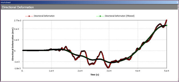
- Display Filter During Solve
This property is applicable only when using Result Tracker filtering in Explicit Dynamics analyses. When set to Yes, it displays filtered data from Result Trackers in the Worksheet at each refresh interval of the Result Tracker. As shown below, a legend is included in the Worksheet to help distinguish the filtered data from the non-filtered data. Typically there are two curves, non-filtered data is displayed in red, and filtered data is displayed in green.
Note: If an error occurs during a solve when using the Mechanical APDL solver, the Solution Information worksheet may point you to files (for example, file.err) in temporary scratch folders whose purpose is for solving only (this is the folder where Ansys actually ran). After the solution, these files are moved back to the project structure, so you may not find them in the scratch folders (or sub-folders).
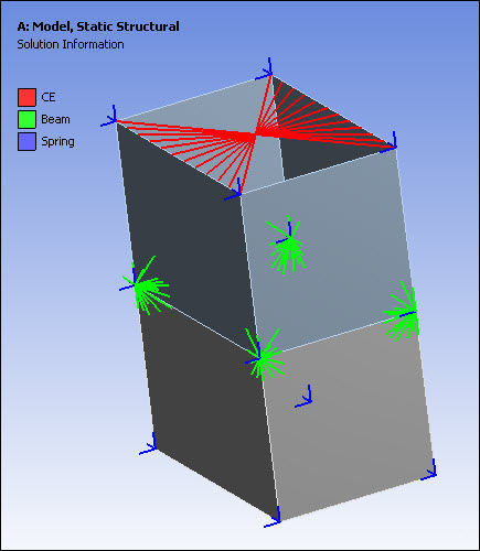
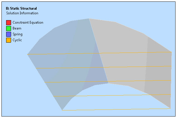
Viewing Finite Element Connections
During the solution, the Mechanical application will sometimes create additional elements or Constrain Equations (CE) for certain objects, such as a remote boundary condition, spot weld, joint, MPC-based contact, or weak springs. So that you might better understand how the boundary conditions are applied, the Mechanical application enables you to "view" these connections after a solution is completed using the properties of the FE Connection Visibility category. Note that this display feature requires a complete solution. For example, connections are not displayed when reading a result file.
The following properties are available in the Details view under the FE Connection Visibility category:
Activate Visibility: Enables control on whether or not the finite element connection data is stored during the solution. If visualization of the finite element connections will never be desired or to maximize performance on extreme models in which many constraint equations exist, this feature can be deactivated by setting the value to No before solving the model. Note that in the case of a multiple step analysis, if constraint equations are present, they will be reported from the first load step. The default value for this property can be changed under Analysis Settings and Solution category of the Options dialog.
Display: Controls which finite element connections to display. The options include:
All FE Connectors (default)
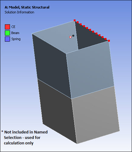
CE Based (As illustrated below, outlined or hollow nodes indicate use for calculation purposes only.)
Beam Based
Weak Springs
None: This option is especially useful to separate the constraint equation connections from the beam connections. The option None is available to assist in avoiding potential performance issues from this feature.
: For a solution containing a Pre-Meshed Cyclic Region, this option displays matching (cyclic) node pairs if they are detected by the solver.
Important: There is a mesh display limitation for this object when your analysis includes a Nonlinear Adaptive Region condition and a remote boundary condition. Currently, this object only shows the base mesh for the geometry, even if it has changed, as it does when a Nonlinear Adaptive Region condition is defined. When you have a Nonlinear Adaptive Region condition combined with a remote boundary condition, the display of the Constrain Equations (CE) is based on the modified mesh, not the displayed mesh (Show Mesh option set to On). That is, the CE display is laid over the base mesh instead of a modified mesh.
Draw Connections Attached To: Based on the availability and visibility of the bodies of your model, this property provides the following options that draw finite element connection annotations for those nodes that are involved in constraint equations.
(default): Nodes attached to available bodies.
: Nodes attached to visible bodies.
Any node-based Named Selections: Nodes in the selected node-based Named Selection.
Line Color: Assigns colors to allow you to differentiate connections. The options include:
Connection Type (default): Displays a color legend that presents one color for constraint equation connections and another color for beam connections.
Manual: Displays a color that you choose.
Color: Appears if Line Color is set to Manual. By clicking in this field, you can choose a color from the color palette.
Visible on Results: When set to Yes (default), the finite element connections are displayed with any result plot (with the exception of a base mesh). When set to No, the connections are displayed only when the Solution Information object is selected.
Line Thickness: Displays the thickness of finite element connection lines in your choice of Single (default), Double, or Triple.
Display Type: enables you to view FE connections as (default) or as . If you wish to view the of a specified Named Selection, the nodes belonging to the Named Selection display as solid colors. Any other associated nodes not belonging to the Named Selection, display with an outline only.
Note: Finite element connection information is not available for Response Spectrum analyses when the Spectrum Type property is set to .