


The Models task page allows you to set various generic model settings.
Important: This feature offers reduced functionality when running Fluent under the Pro capability level.
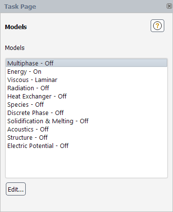
Controls
- Models
contains a listing of the various models available in Ansys Fluent.
You can double-click an item in the Models list to open the corresponding dialog box, or you can select the item in the list and click the Edit... button.
- Multiphase
- selecting this item and clicking the Edit... button opens the Multiphase Model Dialog Box.
- Energy
- selecting this item and clicking the Edit... button opens the Energy Dialog Box.
- Viscous
- selecting this item and clicking the Edit... button opens the Viscous Model Dialog Box.
- Radiation
- selecting this item and clicking the Edit... button opens the Radiation Model Dialog Box.
- Heat Exchanger
- selecting this item and clicking the Edit... button opens the Heat Exchanger Model Dialog Box.
- Species
- selecting this item and clicking the Edit... button opens the Species Model Dialog Box.
The following models are made available, depending on your setup of the Species dialog box.
Spark Ignition - selecting this item and clicking the Edit... button opens the Spark Ignition Dialog Box. Note that spark ignition is only available for transient calculations.
Autoignition - selecting this item and clicking the Edit... button opens the Autoignition Model Dialog Box. Note that autoignition is only available for transient calculations.
Inert - selecting this item and clicking the Edit... button opens the Inert Dialog Box. Note that the inert model is only available when the non-premixed or partially premixed model is selected in the Species Model dialog box, or when a PDF file is read.
NOx - selecting this item and clicking the Edit... button opens the NOx Model Dialog Box. Note that the NOx model is not compatible with premixed combustion.
Soot - selecting this item and clicking the Edit... button opens the Soot Model Dialog Box. Note that none of the soot models are compatible with premixed combustion.
Decoupled Detailed Chemistry - selecting this item and clicking the Edit... button opens the Decoupled Detailed Chemistry Dialog Box.
Reacting Channel Model - selecting this item and clicking the Edit... button opens the Reacting Channel Model Dialog Box.
- Discrete Phase
- selecting this item and clicking the Edit... button opens the Discrete Phase Model Dialog Box.
- Solidification & Melting
- selecting this item and clicking the Edit... button opens the Solidification and Melting Dialog Box.
- Acoustics
- selecting this item and clicking the Edit... button opens the Acoustics Model Dialog Box.
- Structure
- selecting this item and clicking the Edit... button opens the Structural Model Dialog Box.
- Eulerian Wall Film
- selecting this item and clicking the Edit... button opens the Eulerian Wall Film Dialog Box.
- Electric Potential
- selecting this item and clicking the Edit... button opens the Potential/Electrochemistry Dialog Box.
- Edit...
opens the dialog box corresponding to the selected item in the Models list.
For additional information, see the following sections:
- 51.4.1. Multiphase Model Dialog Box
- 51.4.2. Energy Dialog Box
- 51.4.3. Viscous Model Dialog Box
- 51.4.4. Radiation Model Dialog Box
- 51.4.5. View Factors and Clustering Dialog Box
- 51.4.6. Participating Boundary Zones Dialog Box
- 51.4.7. Solar Calculator Dialog Box
- 51.4.8. Heat Exchanger Model Dialog Box
- 51.4.9. Dual Cell Heat Exchanger Dialog Box
- 51.4.10. Set Dual Cell Heat Exchanger Dialog Box
- 51.4.11. Heat Transfer Data Table Dialog Box
- 51.4.12. NTU Table Dialog Box
- 51.4.13. Copy From Dialog Box
- 51.4.14. Ungrouped Macro Heat Exchanger Dialog Box
- 51.4.15. Velocity Effectiveness Curve Dialog Box
- 51.4.16. Core Porosity Model Dialog Box
- 51.4.17. Macro Heat Exchanger Group Dialog Box
- 51.4.18. Species Model Dialog Box
- 51.4.19. Coal Calculator Dialog Box
- 51.4.20. Integration Parameters Dialog Box
- 51.4.21. Flamelet 3D Surfaces Dialog Box
- 51.4.22. Flamelet 2D Curves Dialog Box
- 51.4.23. Unsteady Flamelet Parameters Dialog Box
- 51.4.24. Flamelet Fluid Zones Dialog Box
- 51.4.25. Select Transported Scalars Dialog Box
- 51.4.26. Distribution of Points Dialog Box
- 51.4.27. PDF Table Dialog Box
- 51.4.28. Spark Ignition Dialog Box
- 51.4.29. Set Spark Ignition Dialog Box
- 51.4.30. Autoignition Model Dialog Box
- 51.4.31. Inert Dialog Box
- 51.4.32. NOx Model Dialog Box
- 51.4.33. Soot Model Dialog Box
- 51.4.34. Sticking Coefficients Dialog Box
- 51.4.35. Mechanism Dialog Box
- 51.4.36. Reactor Network Dialog Box
- 51.4.37. Decoupled Detailed Chemistry Dialog Box
- 51.4.38. Reacting Channel Model Dialog Box
- 51.4.39. Reacting Channel 2D Curves Dialog Box
- 51.4.40. Discrete Phase Model Dialog Box
- 51.4.41. DEM Collisions Dialog Box
- 51.4.42. Create Collision Partner Dialog Box
- 51.4.43. Copy Collision Partner Dialog Box
- 51.4.44. Rename Collision Partner Dialog Box
- 51.4.45. DEM Collision Settings Dialog Box
- 51.4.46. Solidification and Melting Dialog Box
- 51.4.47. Acoustics Model Dialog Box
- 51.4.48. Acoustic Sources Dialog Box
- 51.4.49. Acoustic Receivers Dialog Box
- 51.4.50. Basic Shapes Dialog Box
- 51.4.51. Integration Surface Dialog Box
- 51.4.52. Interior Cell Zone Selection Dialog Box
- 51.4.53. Structural Model Dialog Box
- 51.4.54. Eulerian Wall Film Dialog Box
- 51.4.55. Battery Model Dialog Box
- 51.4.56. Standalone Echem Model Dialog Box
- 51.4.57. Potential/Electrochemistry Dialog Box
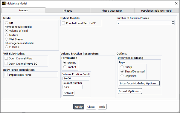
The Multiphase Model dialog box allows you to set parameters for modeling multiphase flow. See Enabling the Multiphase Model – Using the Singhal et al. Expert Cavitation Model for details.
Controls
- Apply
saves the settings specified in the current tab.
Important: When setting up your case, if you have made changes in the current tab, you should click the button to make them effective before moving to the next tab. Otherwise, the relevant models may not be available in the other tabs, and your settings may be lost.
- Models
tab allows you to select a multiphase model and adjust model controls.
- Model
allows you to select one of four multiphase models.
- Off
disables the calculation of multiphase flow.
- Volume of Fluid
enables the VOF model described in Volume of Fluid (VOF) Model Theory in the Theory Guide. See Setting Up the VOF Model for details about using the model. This is available only with the pressure-based solver.
- Mixture
enables the mixture model described in Mixture Model Theory in the Theory Guide. See Setting Up the Mixture Model for details about using the model. This is available only with the pressure-based solver.
- Eulerian
enables the Eulerian model described in Eulerian Model Theory in the Theory Guide. See Setting Up the Eulerian Model for details about using the model. This is available only with the pressure-based solver.
- Wet Steam
enables the wet steam model described in Wet Steam Model Theory in the Theory Guide. See Setting Up the Wet Steam Model for details about using the model.
Important: When General Turbo Interfaces (GTI) are used, available models reduce to Wet Steam only.
For details on the different GTI types, see Blade Row Interaction Modeling.
- Number of Eulerian Phases
allows you to specify the number of phases for the multiphase calculation. You can specify up to 20 phases.
- Coupled Level Set + VOF
allows you to apply an interface tracking method that couples the level set method with the VOF formulation.
- Volume Fraction Parameters
contains parameters related to the VOF and Eulerian model. This section of the dialog box will appear only when Volume of Fluid or Eulerian is the selected Model.
- Formulation
allows you to select the desired volume tracking formulation.
- Explicit
enables the Euler explicit formulation, described in The Explicit Formulation in the Theory Guide. See Choosing Volume Fraction Formulation for more information.
- Implicit
enables the implicit formulation, described in The Implicit Formulation in the Theory Guide. See Choosing Volume Fraction Formulation for more information.
- Volume Fraction Cutoff
specifies a cutoff limit for the volume fraction values. The value that you provide is used as the lower cutoff for the volume fraction. All volume fraction values in the domain below this cutoff value are set to zero. The upper cutoff is calculated as (1.0 - lower cutoff). All volume fraction values above the upper cutoff value are set to 1.0. The default value is 1e-6.
Important: The Volume Fraction Cutoff value can be specified when using the Explicit formulation for volume fraction.
- Courant Number
specifies the maximum Courant number allowed near the free surface. This item will not appear if the Implicit Scheme is selected. See Setting Time-Dependent Parameters for the Explicit Volume Fraction Formulation for details.
- Model Parameters
contains options related to the Mixture model.
- Slip Velocity
enables/disables the calculation of slip velocities for the secondary phases as described in Relative (Slip) Velocity and the Drift Velocity in the Theory Guide. See also Solving a Homogeneous Multiphase Flow.
- Flow Regime Modeling
enables/disables the flow regime modeling as described in Using the Flow Regime Modeling. See also Flow Regime Modeling in the Fluent Theory Guide. This option is available only when Slip Velocity is enabled.
- Regime Transition Modeling
contains options for modeling flow regime transition. This group box is available only with the Eulerian multiphase model.
- Algebraic Interfacial Area Density (AIAD)
allows you to enable the algebraic interfacial area density model and sets its parameters (see Using the Algebraic Interfacial Area Density (AIAD) Model for details).
- Generalized Two Phase Flow (GENTOP)
allows you to enable the GENTOP model and set its parameters (see Steps for Using the GENTOP Model for details).
- Hybrid Models
contains options related to the Eulerian model.
- Dense Discrete Phase Model
allows you to include the Dense Discrete Phase model (see Including the Dense Discrete Phase Model for details). Enabling this model automatically enables the DPM model.
- Multi-Fluid VOF Model
allows you to include the multi-fluid VOF model (see Including the Multi-Fluid VOF Model for details). The multi-fluid VOF model allows the modeling of interface sharpening schemes and free surface flow.
- Sub-Models
is a group box that contains options for the boiling model.
- Boiling Model
when enabled, includes the boiling effects in your simulation (see Including the Boiling Model for details).
- Boiling Options...
opens the Boiling Model dialog box (see Including the Boiling Model for details). This item is available only when the Boiling Model is selected.
- Number of Discrete Phase
allows you to specify the number of discrete phases when the Dense Discrete Phase Model option is enabled.
- Body Force Formulation
contains an additional option for body force calculations.
- Implicit Body Force
enables the implicit body force treatment described in Including Body Forces.
- VOF Sub-Models
contains additional sub-models that can be applied when using the VOF model.
- Open Channel Flow
enables the model to study the effects of open channel flow. See Open Channel Flow in the Theory Guide and Modeling Open Channel Flows for details.
- Open Channel Wave BC
enables the model to set specific parameters for a particular boundary for open channel wave boundaries. This option is not available for axisymmetric cases. See Open Channel Wave Boundary Conditions in the Theory Guide and Modeling Open Channel Wave Boundary Conditions for details.
- Options
contains additional modeling options.
- Interface Modeling
contains settings for how to model interfaces for the VOF model, Mixture multiphase model, and Eulerian with Multi-Fluid VOF enabled. See Interface Modeling Type for details.
- Type
allows you to select the type of interface modeling to be performed. You can choose between Sharp, Dispersed, or a hybrid Sharp/Dispersed when both types of interfaces may be present, or when the interface is mildly sharp. See Interface Modeling Type for more details.
- Interfacial Anti-Diffusion
enables an anti-diffusion treatment at the interface when using the Sharp interface modeling type. This can be used to reduce the effects of numerical diffusion that may occur with coarse meshes, high-aspect ratio cells, or large jumps in cell volume near the interface.
- Interface Modeling Options...
opens the Interface Modeling Options dialog box from which you can enable Zonal Discretization and/or Phase Localized Discretization.
- Expert Options...
opens the Expert Options dialog box which contains settings for VOF time advancement when using the Explicit formulation. Here you can set the Sub-Time Step Calculation Method and enable Solve VOF Every Iteration. See Expert Options for details.
- Phases
tab allows you to define the phases for your simulation. See Steps for Setting Cell Zone Conditions for details.
- Phases
contains a list of all of the phases in the problem from which you can select the phase you want to define or modify. A phase can be a Primary Phase or a Secondary Phase. You cannot change a phase from primary to secondary, or vice versa. Instead, you can redefine the properties of the primary phase to reflect the new phase designated as primary, and redefine the secondary phases accordingly as well.
- Add Phase
adds a new phase in your simulation.
- Delete Phase
deletes the selected phase.
- Phase Setup
is a group box where you can define the properties of the selected primary or secondary phase.
- Name
specifies the name of the phase.
- ID
displays the ID number of the phase. You will need this number only if you are writing a user-defined function. See the separate Fluent Customization Manual for details about writing user-defined functions for multiphase applications.
- Phase Material
contains a drop-down list of available materials, from which you can select the appropriate one for this phase. This control is not available for the DDPM.
- Edit...
opens the Edit Material Dialog Box for the selected Phase Material, where you can modify its properties.
- Granular
(secondary phase) indicates whether or not this is a solid phase. This item appears only for the Eulerian model.
- Packed Bed
(secondary phase only) indicates whether or not the granular phase is a packed bed. This option appears only if Granular is selected.
- Interfacial Area Concentration
(secondary phase only) is used to predict mass, momentum and energy transfers through the interface between the phases. See Interfacial Area Concentration in the Theory Guide for details. This option is not available if Granular is selected.
- Granular Temperature Model
(secondary phase only) lists the granular temperature models.
- Phase Property
enables phase property model for granular temperature.
- Partial Differential Equation
enables partial differential equation model for granular temperature. See Granular Temperature in the Theory Guide for details.
- Volume Fraction Approaching Packing Limit
prevents the unlimited accumulation of particles, which are operating at packing limit conditions. This options is available only for the DDPM.
- Transition Factor
is specified as either a constant or a user-defined function. The default value is assumed to be 0.75, which corresponds to the closest sphere packing for monosized spheres (a factor of 4/3). In other words, the transition criterion is based on the local particle volume fraction of the given discrete phase and is specified as a factor multiplied by the maximum packing limit (also a user specified value). This control appears only when Volume Fraction Approaching Packing Limit is selected.
- Diameter
(secondary phase only) specifies the diameter of the particles. You can select constant in the drop-down list and specify a constant value, or select user-defined to use a user-defined function. See the separate Fluent Customization Manual for details about user-defined functions. The Diameter appears for both the mixture model and the Eulerian model. This control is not available for the DDPM.
- Granular Properties
(secondary phase only) contains a list of granular phase-specific properties. This section of the dialog box will not appear for the VOF model. This list is only if Granular is selected.
- Granular Viscosity
specifies the kinetic part of the granular viscosity of the particles (
 in Equation 14–362 in the Theory Guide). You can select
constant (the default) in the drop-down list and specify a
constant value, select syamlal-obrien to compute the value using
Equation 14–364
in the Theory Guide, select
gidaspow to compute the value using Equation 14–365 in the Theory Guide, or select
user-defined to use a user-defined function. Note the
following:
in Equation 14–362 in the Theory Guide). You can select
constant (the default) in the drop-down list and specify a
constant value, select syamlal-obrien to compute the value using
Equation 14–364
in the Theory Guide, select
gidaspow to compute the value using Equation 14–365 in the Theory Guide, or select
user-defined to use a user-defined function. Note the
following: If you select filtered for Drag Coefficient, then Granular Viscosity is set automatically to filtered. The granular viscosity will be calculated as described in The Filtered Two-Fluid Model in the Fluent Theory Guide.
If you select user-defined, your user-defined function must include both the kinetic portion and the collisional portion of the viscosity in the value it returns.
- Granular Bulk Viscosity
specifies the solids bulk viscosity (
 in Equation 14–195 in the Theory Guide). You can select
constant (the default) in the drop-down list and specify a
constant value, select lun-et-al to compute the value using
Equation 14–366 in the
Theory Guide, or select
user-defined to use a user-defined function. Note that if you
select filtered for Drag Coefficient, then
Granular Bulk Viscosity is set to zero automatically.
in Equation 14–195 in the Theory Guide). You can select
constant (the default) in the drop-down list and specify a
constant value, select lun-et-al to compute the value using
Equation 14–366 in the
Theory Guide, or select
user-defined to use a user-defined function. Note that if you
select filtered for Drag Coefficient, then
Granular Bulk Viscosity is set to zero automatically.- Frictional Viscosity
specifies a shear viscosity based on the viscous-plastic flow (
 in Equation 14–362 in the Theory Guide). By default, the frictional viscosity is
neglected, as indicated by the default selection of none in the
drop-down list. If you want to include the frictional viscosity, you can select
constant and specify a constant value, select
schaeffer to compute the value using Equation 14–367 in the Theory Guide, or select
user-defined to use a user-defined function.
in Equation 14–362 in the Theory Guide). By default, the frictional viscosity is
neglected, as indicated by the default selection of none in the
drop-down list. If you want to include the frictional viscosity, you can select
constant and specify a constant value, select
schaeffer to compute the value using Equation 14–367 in the Theory Guide, or select
user-defined to use a user-defined function.- Angle Of Internal Friction
specifies a constant value for the angle
 used in Schaeffer’s expression for frictional viscosity
(Equation 14–367 in
the Theory Guide). This
parameter is relevant only if you have selected schaeffer or
user-defined for the Frictional
Viscosity.
used in Schaeffer’s expression for frictional viscosity
(Equation 14–367 in
the Theory Guide). This
parameter is relevant only if you have selected schaeffer or
user-defined for the Frictional
Viscosity.- Frictional Pressure
specifies the pressure gradient term,
 , in the granular-phase momentum equation. Choose
none to exclude frictional pressure from your calculation,
johnson-et-al to apply Equation 14–371 in the Theory Guide, syamlal-et-al to apply
Equation 14–268 in the Theory Guide,
based-ktgf, where the frictional pressure is defined by the
kinetic theory [38]. The solids pressure tends to a
large value near the packing limit, depending on the model selected for the radial
distribution function. You must hook a user-defined function when selecting the
user-defined option. See the separate Fluent Customization Manual for information on hooking a UDF.
, in the granular-phase momentum equation. Choose
none to exclude frictional pressure from your calculation,
johnson-et-al to apply Equation 14–371 in the Theory Guide, syamlal-et-al to apply
Equation 14–268 in the Theory Guide,
based-ktgf, where the frictional pressure is defined by the
kinetic theory [38]. The solids pressure tends to a
large value near the packing limit, depending on the model selected for the radial
distribution function. You must hook a user-defined function when selecting the
user-defined option. See the separate Fluent Customization Manual for information on hooking a UDF.- Frictional Modulus
can be set as derived, or as a user-defined function. This is defined as Equation 26–17.
- Friction Packing Limit
specifies a threshold volume fraction at which the frictional regime becomes dominant. The default value is 0.61.
- Granular Conductivity
specifies the solids conductivity. You can select syamlal-obrien, gidaspow, constant or user-defined.
- Granular Temperature
specifies temperature for the solids phase and is proportional to the kinetic energy of the random motion of the particles. You can choose the algebraic, constant, dpm-averaged,or user-defined option. dpm-averaged is available only when using the Dense Discrete Phase Model (DDPM). Note that if you select filtered for Drag Coefficient, then Granular Temperature is set to zero automatically.
- Solids Pressure
specifies the pressure gradient term,
 , in the granular-phase momentum equation. Choose either the
lun-et-al, the syamlal-obrien, the
ma-ahmadi, or the user-defined option.
Note that if you select filtered for Drag
Coefficient, then Solids Pressure is set
automatically to filtered. The solid pressure will be calculated
as described in The Filtered Two-Fluid Model in the Fluent Theory Guide.
, in the granular-phase momentum equation. Choose either the
lun-et-al, the syamlal-obrien, the
ma-ahmadi, or the user-defined option.
Note that if you select filtered for Drag
Coefficient, then Solids Pressure is set
automatically to filtered. The solid pressure will be calculated
as described in The Filtered Two-Fluid Model in the Fluent Theory Guide.- Radial Distribution
specifies a correction factor that modifies the probability of collisions between grains when the solid granular phase becomes dense. Choose either the lun-et-al, the syamlal-obrien, the ma-ahmadi, the arastapour, or a user-defined option. Note that if filtered is selected for Drag Coefficient, then Radial Distribution is set automatically to filtered. In the simulation, the radial distribution will be set to zero since the filtered two-fluid model is not based on kinetic theory.
- Elasticity Modulus
is defined as

(51–1)
with
 .
.Choose either the derived or user-defined options.
- Packing Limit
specifies the maximum volume fraction for the granular phase. For monodispersed spheres the packing limit is about 0.63, which is the default value in Ansys Fluent. In polydispersed cases, however, smaller spheres can fill the small gaps between larger spheres, so you may need to increase the maximum packing limit.
- Phase State
is a group box where you can select either Liquid or Gas phase state. This item is available only when Flow Regime Modeling is selected in the Models tab (Model Parameters group box).
- Phase Morphology
is a group box where you can select from the following phase morphology options:
Continuous
Dispersed (secondary phase only)
Hybrid
This item is available only when Flow Regime Modeling is selected in the Models tab (Model Parameters group box).
- Interfacial Area Concentration Properties
(secondary phase only) contains a list of phase-specific properties. This list is available only if Interfacial Area Concentration is selected. This section of the dialog box will not appear for the VOF, mixture, or DDPM multiphase models.
- Min/Max Diameter
are the limits of the bubble diameters.
- Breakage Kernel
allows you to specify the breakage kernel. You can select none, constant, hibiki-ishii, ishii-kim, yao-morel, or user-defined. The three options, hibiki-ishii, ishii-kim, and yao-morel are described in detail in Interfacial Area Concentration in the Theory Guide.
- Coalescence Kernel
allows you to specify the coalescence kernel. You can select none, constant, hibiki-ishii, ishii-kim, yao-morel, or user-defined. The three options, hibiki-ishii, ishii-kim, and yao-morel are described in detail in Interfacial Area Concentration in the Theory Guide.
- Nucleation Rate
is a source term for the interfacial area concentration that models the rate of formation of the dispersed phase. You can choose from constant or user-defined. If the Boiling Model option is enabled when using the Eulerian multiphase model, you can also select yao-morel. The yao-morel option is described in Yao-Morel Model in the Theory Guide.
- Surface Tension
specifies the attractive forces between the interfaces.
- Critical Weber Number
will need to be specified if you selected yao-morel for the Breakage Kernel.
- Dissipation Function
gives you the option to choose the formula which calculates the dissipation rate used in the hibiki-ishii and ishii-kim models. You can choose constant, wu-ishii-kim, fluent-ke, and user-defined for the dissipation function.
- Hydraulic Diameter
is the value used in Equation 26–19. This is available when the wu-ishii-kim formulation is selected as the Dissipation Function. .
- Phase Interaction
tab allows you to define the interaction between phases.
- Interaction Domain ID
displays the ID number of the interaction domain. You will need this number only if you are writing a user-defined function. See the separate Fluent Customization Manual for details about writing user-defined functions for multiphase applications.
- Forces
tab allows you to specify forces acting between the phases.
- Phase Pairs
is a list of all of the phase pairs in the problem from which you can select the pair and define the forces between the phases.
- Global Options
contains controls that apply along phase interface in each pair of phases.
- Shaver-Podowski Lift Correlation
(Eulerian Multiphase model only) when enabled, improves the accuracy of the prediction of the void peak near the wall and overall robustness for cases where lift force, turbulent dispersion, and wall lubrication are included. See Including the Lift Correlation for more information.
- Virtual Mass Implicit Options
specifies what form of the implicit method to use. Default models the entire virtual mass force while Option 2 and Option 3 model truncated expressions which may further improve convergence. This option appears only when the Virtual Mass Coefficient is set to a nonzero value in the Force Setup group box.
- Surface Tension Force Modeling
includes the effects of surface tension along the fluid-fluid interface.
- Model
contains two surface tension models from which to choose.
- Continuum Surface Force
adds the surface tension to the VOF calculation, which results in a source term in the momentum equation. This method is available only for the VOF and Eulerian models.
- Continuum Surface Stress
is an alternative way to modeling surface tension in a conservative manner compared to the continuum surface force method. This method is available only for the VOF and Eulerian models.
- Adhesion Options
contains options to include wall and jump adhesion.
- Wall Adhesion
enables the specification of a wall adhesion angle. (The angle itself, as defined in Figure 26.21: Measuring the Contact Angle, will be specified in the Wall Dialog Box.)
- Jump Adhesion
enables the treatment of the contact angle specification at the porous jump boundary. (The angle itself will be specified in the Porous Jump Dialog Box.)
- Force Setup
contains a list of forces specified for the selected pair of phases. By default, the forces in the Force Setup group box are set to none. Depending on your case, the following forces can be defined:
Drag Coefficient: You can select the appropriate drag function from the Coefficient drop-down list and drag factor from the Modification drop-down list. See Specifying the Drag Function and Drag Modification for information about the available options. This input is available only for the Eulerian and mixture models only.
Lift Coefficient: Specifies the lift function for each pair of phases. See Defining the Phases for the Eulerian Model for information about the available options. This input is available only for the Eulerian model.
Wall Lubrication: Specifies the wall lubrication model for each primary-secondary phase pair. See Including the Wall Lubrication Force for information about the available options. This input is available only for Eulerian two-phase flows with a non-granular phase.
Turbulent Dispersion: Specifies the turbulent dispersion model for each primary-secondary phase pair. See Including the Turbulent Dispersion Force for information about the available options. This input is available only for the Eulerian model.
Turbulence Interaction: Specifies the turbulence interaction model for each primary-secondary phase pair. See Including Turbulence Interaction Source Terms for information about the available options. This input is available only for the Eulerian model.
Virtual Mass Coefficient: Specifies the virtual mass coefficient for each pair of phases. See Including the Virtual Mass Force for details. This input is available only for the Eulerian model.
Slip Velocity: Specifies the slip velocity function for each secondary phase with respect to the primary phase. See Defining the Phases for the Mixture Model for information about the available options. This input is available only for the mixture multiphase model.
Surface Tension Coefficients: Specify the surface tension coefficient,
 in Equation 14–23 and
Equation 12–58 in the Theory Guide, for each pair of phases.
See Defining the Phases for the VOF Model for details. This input is available
only for the Eulerian model.
in Equation 14–23 and
Equation 12–58 in the Theory Guide, for each pair of phases.
See Defining the Phases for the VOF Model for details. This input is available
only for the Eulerian model.Restitution Coefficient: Specifies the restitution coefficient for collisions between each pair of granular phases, and for collisions between particles of the same granular phase. It is relevant only if two or more granular phases are involved. See Defining the Phases for the Eulerian Model for information about the available options.
- Heat, Mass, Reactions
tab contains the following tabs:
- Heat
tab displays the Heat Transfer Coefficient inputs. See Including Heat Transfer Effects for information about the available options. This tab is active only for the Eulerian model when the energy equation is active.
- Heat Transfer Coefficient
specifies the heat transfer coefficient function between each pair of phases. See Including Heat Transfer Effects for information about the available options.
- Mass
tab displays the Mass Transfer Function inputs.
- Number of Mass Transfer Mechanisms
specifies the number of mass transfer mechanisms in your simulation. See Including Mass Transfer Effects for information about the available options.
- Reactions
tab allows you to define multiple heterogeneous reactions and stoichiometry.
- Total Number of Heterogeneous Reactions
specifies the total number of reactions (volumetric reactions, wall surface reactions, and particle reactions). See Specifying Heterogeneous Reactions for information about the available options.
- Heterogeneous Stiff Chemistry Solver
is used in inter-phase reaction mechanisms containing numerically stiff reactions. This option can improve convergence and is available for transient Eulerian multiphase simulations.
- Reaction Name
allows you to enter a name for the reaction.
- ID
enables you to set the reaction ID for each reaction.
- Number of Reactants
allows you to specify the number of reactants that are involved in the reaction.
- Number of Products
allows you to specify the number of products that are involved in the reaction.
- Phase
drop-down list allows you to select the phase that is involved in the reaction.
- Species
drop-down list allows you to select the species.
- Stoich. Coefficient
allows you to set the stoichiometric coefficient.
- Reaction Rate Function
allows you to choose rate exponents for an Arrhenius-type reaction, a user-defined function, or a population balance mechanism for the reaction rate.
- Interfacial Area
tab displays the Interfacial Area settings to predict interfacial area between the phases. This tab appears only for the Mixture multiphase model with interphase mass transfer and the Eulerian multiphase model. See Defining the Algebraic Interfacial Area Concentration and Using an Algebraic Interfacial Area Model for information about the available options.
- Discretization
tab allows you to use the diffusive and anti-diffusive discretization procedure across the distinct interfaces.
- Phase Localized Compressive Scheme
enables the compressive discretization scheme in Ansys Fluent, where the degree of diffusion/sharpness is controlled through the value of the slope limiters. This item will appear only for the VOF model and for the Eulerian model with Multi-Fluid VOF Model enabled.
- Slope Limiters
are values equating to specific discretization schemes. For each pair of phases, you can enter a value of 0, 1, or 2, or any value between 0 and 2. Depending on the value you use, first order upwind, second order upwind, compressive, or the blended scheme will be applied. Refer to Table 26.11: Slope Limiter Discretization Scheme to equate each value of the slope limiter with a discretization scheme. For more information, refer to Discretizing Using the Phase Localized Compressive Scheme.
- Model Transition
displays the VOF-to-DPM Model Transition inputs. This tab is available only when a DPM injection is set as described in Setting up the VOF-to-DPM Model Transition.
- Number of Model Transition Mechanisms
specifies the number of VOF-to-DPM model transition mechanisms in your simulation. See Setting up the VOF-to-DPM Model Transition for information about the available options.
- Population Balance
tab contains controls for setting population balance simulations. This tab is displayed for the mixture and Eulerian multiphase models. See Population Balance Model for details.
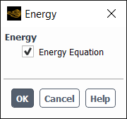
The Energy dialog box allows you to set parameters related to energy or heat transfer in your model.
Controls
- Energy
contains inputs related to the modeling of energy.
- Energy Equation
enables/disables the calculation of energy in the model.
- Energy Modes
contains inputs related to the alternative energy modeling modes.
- Two-Temperature Model
enables/disables the Two-Temperature Model. Only available for the density-based solver.
The Viscous Model dialog box allows you to set parameters for inviscid, laminar, and turbulent flow. See Steps in Using a Turbulence Model for details about using this dialog box.
Important: This feature offers reduced functionality when running Fluent under the Pro capability level.
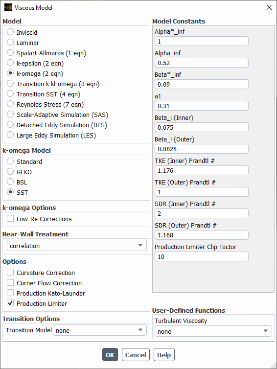
Controls
- Model
contains options for specifying the viscous model.
- Inviscid
specifies inviscid flow.
- Laminar
specifies laminar flow.
- Spalart-Allmaras
specifies turbulent flow to be calculated using the Spalart-Allmaras model. (See Spalart-Allmaras Model in the Theory Guide for background about this model. See Setting Up the Spalart-Allmaras Model for details about using this model.)
- k-epsilon
specifies turbulent flow to be calculated using one of three
 -
- models. (See Standard, RNG, and Realizable k-ε Models in
the Theory Guide for background about this model. See Setting Up the k-ε Model for details about using this model.)
models. (See Standard, RNG, and Realizable k-ε Models in
the Theory Guide for background about this model. See Setting Up the k-ε Model for details about using this model.)- k-omega
specifies turbulent flow to be calculated using one of two
 -
- models. (See Standard, BSL, and SST k-ω Models in
the Theory Guide for background about these models. See Setting Up the k-ω Model for details about using this model.)
models. (See Standard, BSL, and SST k-ω Models in
the Theory Guide for background about these models. See Setting Up the k-ω Model for details about using this model.)- Transition k-kl-omega
specifies turbulent flow to be calculated using the Transition
 -
- -
- model. (See k-kl-ω Transition Model in the Theory Guide for
background about this model. See Setting Up the Transition k-kl-ω Model for details about using this
model.)
model. (See k-kl-ω Transition Model in the Theory Guide for
background about this model. See Setting Up the Transition k-kl-ω Model for details about using this
model.)- Transition SST
specifies turbulent flow to be calculated using the Transition SST model. (See Transition SST Model in the Theory Guide for background about this model. See Setting Up the Transition SST Model for details about using this model.)
- Reynolds Stress
specifies turbulent flow to be calculated using the RSM. (See Reynolds Stress Model (RSM) in the Theory Guide for background about this model. See Setting Up the Reynolds Stress Model for details about using this model.)
- Scale-Adaptive Simulation (SAS)
specifies turbulent flow to be calculated using the SAS model in combination with the SST
 -
- model. (See Scale-Adaptive Simulation (SAS) Model in the Theory Guide for
background about this model. See Setting Up Scale-Adaptive Simulation (SAS) Modeling for details about using this model.)
model. (See Scale-Adaptive Simulation (SAS) Model in the Theory Guide for
background about this model. See Setting Up Scale-Adaptive Simulation (SAS) Modeling for details about using this model.)- Detached Eddy Simulation
specifies turbulent flow to be calculated using the DES model. (See Detached Eddy Simulation (DES) in the Theory Guide for background about this model. See Setting Up the Detached Eddy Simulation Model for details about using this model.)
- Large Eddy Simulation
(3D only) specifies turbulent flow to be calculated using the LES model. (See Large Eddy Simulation (LES) Model in the Theory Guide for background about this model. See Setting Up the Large Eddy Simulation Model for details about using this model.)
- Spalart-Allmaras Production
contains options for the Spalart-Allmaras model. This portion of the dialog box will appear only if Spalart-Allmaras is selected as the Model.
- Vorticity-Based
selects the vorticity-based calculation of the deformation tensor
 (see Equation 4–22 in the Theory Guide).
- Strain/Vorticity-Based
selects the strain/vorticity-based calculation of the deformation tensor
 (see Equation 4–24 in the Theory Guide).
- k-epsilon Model
contains options for specifying which of the
 -
- models is to be used.
This portion of the dialog box will appear only if k-epsilon is selected as the Model.
models is to be used.
This portion of the dialog box will appear only if k-epsilon is selected as the Model.- Standard
selects the standard
 -
- model, described in Standard k-ε Model in the Theory Guide and Setting Up the k-ε Model.
- RNG
selects the RNG
 -
- model, described in RNG k-ε Model. in the Theory Guide and Setting Up the k-ε Model.
- Realizable
selects the realizable
 -
- model, described in Realizable k-ε Model
in the Theory Guide and Setting Up the k-ε Model.
model, described in Realizable k-ε Model
in the Theory Guide and Setting Up the k-ε Model.
- RNG Options
specifies parameters that affect the solution of problems solved with the RNG
 -
- model. This portion of the dialog
box will appear only if RNG is selected as the k-epsilon Model.
model. This portion of the dialog
box will appear only if RNG is selected as the k-epsilon Model.- Differential Viscosity Model
specifies whether or not the low-Reynolds-number RNG modifications to turbulent viscosity should be included. By default, this option is turned off. It is likely to have an effect only when the near-wall regions in the domain are well resolved in terms of mesh density. See Differential Viscosity Modification for details.
- Swirl Dominated Flow
specifies whether or not the RNG modification to turbulent viscosity for swirling flows should be included. This option is available only in 3D and 2D axisymmetric swirl solvers, and it can yield improved predictions when solving flows with significant swirl. See Swirl Modification for details.
- k-omega Model
contains options for specifying which of the
 -
- models is to be used. This
portion of the dialog box will appear only if k-omega is selected as the Model.
models is to be used. This
portion of the dialog box will appear only if k-omega is selected as the Model.- Standard
selects the standard
 -
- model, described in Standard k-ω Model in the Theory Guide and Setting Up the k-ω Model.
- GEKO
selects the generalized
- model, described in Generalized k-ω (GEKO) Model in the Theory Guide and Setting up the Generalized k-ω (GEKO) Model.- BSL
selects the baseline (BSL)
 -
- model, described in Baseline (BSL) k-ω Model in
the Theory Guide and Setting Up the k-ω Model.
model, described in Baseline (BSL) k-ω Model in
the Theory Guide and Setting Up the k-ω Model.- SST
selects the shear-stress transport (SST)
 -
- model, described in Shear-Stress Transport (SST) k-ω Model in
the Theory Guide and Setting Up the k-ω Model.
model, described in Shear-Stress Transport (SST) k-ω Model in
the Theory Guide and Setting Up the k-ω Model.
- k-omega Options
specifies parameters that affect the solution of problems solved with the
 -
- models. This portion of the dialog box
will appear only if k-omega is selected as the Model.
models. This portion of the dialog box
will appear only if k-omega is selected as the Model.- Low-Re Corrections
specifies whether corrections that improve the accuracy in predicting low Reynolds number flows should be included. This option is available only for the
 -
- models and the stress-omega RSM model.
See Low-Re Corrections for details.
models and the stress-omega RSM model.
See Low-Re Corrections for details.- Shear Flow Corrections
specifies whether corrections that improve the accuracy in predicting free shear flows should be included. This option is available only for the standard
 -
- model and the stress-omega RSM model. See Shear Flow Corrections for details.
- Transition SST Options
allows you to include the Roughness Correlation of rough walls as described in Transition SST and Rough Walls in the Theory Guide.
- Roughness Correlation
when enabled allows you to specify the Geometric Roughness Height as a constant value.
- Reynolds-Stress Model
specifies the various Reynolds stress models (RSM).
- Linear Pressure-Strain
enables the linear pressure-strain model. See Linear Pressure-Strain Model in the Theory Guide for details.
- Quadratic Pressure-Strain
enables the quadratic pressure-strain model for superior performance in a range of basic shear flows, including plane strain, rotating plane shear, and axisymmetric expansion/contraction. See Quadratic Pressure-Strain Model in the Theory Guide for details. Note that this option cannot be used with the Wall Reflection Effects option or the Enhanced Wall Treatment.
- Stress-Omega
enables a stress-transport model that is based on the omega equations and LRR model [173]. This model is ideal for modeling flows over curved surfaces and swirling flows. See Stress-Omega Model in the Theory Guide for details.
- Stress-BSL
enables a linear model for the pressure-strain term like the Stress-Omega model, but solves the scale equation from the baseline (BSL)
 -
- model, and thus removes the free-stream
sensitivity observed with the Stress-Omega model.
Like the Stress-Omega model, it is recommended
for modeling flows over curved surfaces and swirling flows. See Stress-BSL Model in the Theory Guide for details.
model, and thus removes the free-stream
sensitivity observed with the Stress-Omega model.
Like the Stress-Omega model, it is recommended
for modeling flows over curved surfaces and swirling flows. See Stress-BSL Model in the Theory Guide for details.
- Reynolds-Stress Options
specifies parameters that affect the solution of problems solved with the Reynolds stress model. This portion of the dialog box will appear only if Reynolds Stress is selected as the Model.
- Wall BC from k Equation
enables the explicit setting of boundary conditions for the Reynolds stresses near the walls, using the values computed with Equation 4–260 in the Theory Guide. See Solving the k Equation to Obtain Wall Boundary Conditions for details. This option is on by default.
- Wall Reflection Effects
enables the calculation of the component of the pressure strain term responsible for the redistribution of normal stresses near the wall. See Including the Wall Reflection Term for details. Note that this option is not available if you have enabled the Quadratic Pressure-Strain Model.
- RANS Model
contains options for the subgrid-scale model used by the Detached Eddy Simulation Model. This portion of the dialog box will appear only if Detached Eddy Simulation Model is selected as the Model.
- Spalart-Allmaras
enables the Spalart-Allmaras RANS model. See Detached Eddy Simulation (DES) in the Theory Guide for details.
- Realizable k-epsilon
enables the Realizable
 -
- RANS model. See Detached Eddy Simulation (DES) in the Theory Guide for
details.
RANS model. See Detached Eddy Simulation (DES) in the Theory Guide for
details.- SST k-omega
enables the SST
 -
- RANS Model. See Detached Eddy Simulation (DES) in the Theory Guide for
details.
RANS Model. See Detached Eddy Simulation (DES) in the Theory Guide for
details.
- DES Options
contain the option to include a delayed Detached Eddy Simulation.
- Delayed DES
is useful for RANS meshes with high aspect ratios in the boundary layer. This option preserves the RANS model throughout the boundary layer. (See Delayed Detached Eddy Simulation (DDES) for details.)
- Subgrid-Scale Model
contains options for the subgrid-scale model used by the LES model. This portion of the dialog box will appear only if Large Eddy Simulation is selected as the Model.
- Smagorinsky-Lilly
selects the Smagorinsky-Lilly subgrid-scale model described in Subgrid-Scale Models in the Theory Guide.
- WALE
selects the Wall-Adapting local Eddy-Viscosity model described in Wall-Adapting Local Eddy-Viscosity (WALE) Model in the Theory Guide.
- WMLES
selects the algebraic Wall-Modeled LES model described in Algebraic Wall-Modeled LES Model (WMLES) in the Theory Guide.
- WMLES S-Omega
selects the algebraic Wall-Modeled LES
 -
- model described in Algebraic WMLES S-Omega Model Formulation in the Theory Guide.
- Kinetic-Energy Transport
selects the dynamic kinetic energy subgrid-scale model described in Dynamic Kinetic Energy Subgrid-Scale Model in the Theory Guide.
- LES Model Options
contains options for the Large Eddy Simulation model. This portion of the dialog box will appear only if Large Eddy Simulation is selected as the Model.
- Dynamic Stress
enables the dynamic stress model. It is available for selection when the Smagorinsky-Lilly is selected, and is enabled (and cannot be disabled) when the Kinetic-Energy Transport is selected.
- Dynamic Energy Flux
enables the dynamic energy flux model. It is available when the LES model option Dynamic Stress is enabled.
- Dynamic Scalar Flux
enables the dynamic computation of turbulent Sc (
 in Equation 8–5
in the Theory Guide). See Definition of the Mixture Fraction in the Theory
Guide for details. It is available when the LES model
option Dynamic Stress is enabled.
in Equation 8–5
in the Theory Guide). See Definition of the Mixture Fraction in the Theory
Guide for details. It is available when the LES model
option Dynamic Stress is enabled.- Dynamic Fvar
enables the dynamic mixture fraction variance model. It is available when Non-Premixed Combustion or Partially Premixed Combustion is selected in the Species Model Dialog Box. See The Non-Premixed Model for LES in the Theory Guide for details.
- Near-Wall Treatment
specifies the near-wall treatment to be used for modeling turbulence. See Near-Wall Treatments for Wall-Bounded Turbulent Flows in the Theory Guide for details about the available methods. This portion of the dialog box will appear if k-epsilon or Reynolds Stress is selected as the Model.
- Standard Wall Functions
enables the use of standard wall functions (described in Standard Wall Functions in the Theory Guide).
- Scalable Wall Functions
enables the use of scalable wall functions (described in Scalable Wall Functions in the Theory Guide).
- Non-Equilibrium Wall Functions
enables the use of non-equilibrium wall functions (described in Non-Equilibrium Wall Functions in the Theory Guide).
- Enhanced Wall Treatment
enables the use of the enhanced wall treatment (described in Enhanced Wall Treatment ε-Equation (EWT-ε) in the Theory Guide). Note that this option will not appear if you have enabled the Quadratic Pressure-Strain Model under Reynolds-Stress Options.
- Menter-Lechner
enables the use of the Menter-Lechner near-wall treatment (described in Menter-Lechner ε-Equation (ML-ε) in the Theory Guide). Note that this option is only available when k-epsilon is selected for the Model.
- User-Defined Wall Functions
enables you to hook a user-defined function, used to define the Law of the Wall. See User-Defined Wall Functions in the Theory Guide for more information.
- Enhanced Wall Treatment Options
allows you to include pressure gradient or thermal effects in the calculation. See Near-Wall Treatments for Wall-Bounded Turbulent Flows in the Theory Guide.
- Pressure Gradient Effects
enables the effect of pressure gradient.
- Thermal Effects
enables thermal effects in the calculation. This option appears only if the energy equation is enabled.
- Options
contains general options for viscous modeling.
- Viscous Heating
(if enabled) includes the viscous dissipation terms in the energy equation. This option is recommended when you are solving a compressible flow. Note that this option is always turned on when one of the density-based solvers is used; you will not be able to turn it off.
- Low-Pressure Boundary Slip
includes slip boundary conditions for velocity and temperature for modeling fluid flow at very low pressures as in semiconductor fabrication devices. See Slip Boundary Formulation for Low-Pressure Gas Systems in the Theory Guide. This option is available only for laminar flows.
- Buoyancy Effects
enables the inclusion of buoyancy effects. See Including Buoyancy Effects on Turbulence for details. Only available for non-isothermal flow and when a nonzero gravitational acceleration has been specified in the Operating Conditions Dialog Box.
- Curvature Correction
when enabled, modifies the turbulence production term to sensitize the standard eddy-viscosity models to the effects of streamline curvature and system rotation. This is available for the Spalart-Allmaras, k-epsilon, k-omega, Transition SST, Scale-Adaptive Simulation, and Detached Eddy Simulation with the SST k-omega model.
- Curvature Correction Options
Includes options related to curvature corrections.
- CCURV
specifies a coefficient used in the curvature correction term to influence the strength of the curvature correction if needed for a specific flow. Can be a constant or specified via UDF.
- Corner Flow Correction
when enabled, accounts for secondary flows found in rectangular channels, pipes of non-circular cross-section, and wing-body-junction type geometries in the plane normal to the main flow direction into the corner along the bisector.
- Corner Flow Correction Options
Includes options related to corner flow corrections.
- CCORNER
Sets the strength of the quadratic term of the corner flow correction. The default value is 1. Can be a constant or specified via UDF.
- Compressibility Effects
when enabled, can improve the prediction of free shear layers at high Mach numbers. This is available when the compressible form of the ideal gas law or the real-gas model is activated for k-epsilon, k-omega, Transition k-kl-omega, Reynolds Stress, Scale-Adaptive Simulation, and Detached Eddy Simulation with the Realizable k-epsilon model. For details, see Model Enhancements.
- Mixture Drift Force
includes the effect of turbulent drift velocity when using the Mixture model. See Modeling Turbulence. Note that this option is only available when using the Mixture model with Slip Velocity enabled in the Multiphase Model dialog box. See Including Mixture Drift Force.
- Production Kato-Launder
when enabled, the Kato-Launder modification for the production term limits the production term in the turbulence equation. For details see, Production Limiters for Two-Equation Models in the Fluent Theory Guide.
- Production Limiter
when enabled, limits the production term in the turbulence equation. For details, see Production Limiters for Two-Equation Models in the Fluent Theory Guide.
- Transition Options
contains options for transition modeling.
- Transition Model
selects the transition model. You can enable the gamma-transport-eqn model (also known as the Intermittency Transition model). For details, see Intermittency Transition Model in the Theory Guide.
- Include Crossflow Transition
includes the effects of crossflow instability. For details, see Transport Equations for the Intermittency Transition Model in the Theory Guide.
- Turbulence Multiphase Model
contains options for multiphase turbulence models. This portion of the dialog box will appear if Eulerian is selected as the Model in the Multiphase Model Dialog Box.
- Mixture
specifies the (default) mixture turbulence model.
- Dispersed
specifies the dispersed turbulence model.
- Per Phase
specifies the calculation of a set of turbulence equations for each phase.
See Turbulence Models in the Theory Guide for details about the available multiphase turbulence models.
- GEKO Options
contains options for the GEKO model.
- Wall Distance Free
Selects the wall distance free version of the GEKO model.
- CSEP
Specifies
 - parameter to optimize flow separation from smooth surfaces.
 - CNW
Specifies
 - parameter to optimize flow in non-equilibrium near wall regions (such
as heat transfer or
- parameter to optimize flow in non-equilibrium near wall regions (such
as heat transfer or  ).
).- CMIX
Specifies
 - parameter to optimize strength of mixing in free shear flows.
- CJET
Specifies
 - parameter to optimize free shear layer mixing (optimize free jets
independent of mixing layer).
- parameter to optimize free shear layer mixing (optimize free jets
independent of mixing layer).- Blending Function
Specifies the blending function,
 , which deactivates these parameters inside boundary layers.
See Generalized k-ω (GEKO) Model in the Fluent Theory Guide for details about the GEKO model options.
- Model Constants
contains constants used in the equations for turbulence. See Spalart-Allmaras Model, Standard k-ε Model, RNG k-ε Model, k-kl-ω Transition Model, Transition SST Model, Realizable k-ε Model, Reynolds Stress Model (RSM), Standard k-ω Model, Shear-Stress Transport (SST) k-ω Model, and Large Eddy Simulation (LES) Model in the Theory Guide for details about these constants.
- Cb1
(only for the Spalart-Allmaras model) is the constant
 in Equation 4–19 in
the Theory Guide.
in Equation 4–19 in
the Theory Guide.- Cb2
(only for the Spalart-Allmaras model) is the constant
 in Equation 4–15 in the Theory Guide.
- Cv1
(only for the Spalart-Allmaras model) is the constant
 in Equation 4–17 in the Theory Guide.
- Cw2
(only for the Spalart-Allmaras model) is the constant
 in Equation 4–28 in the Theory Guide.
- Cw3*
(* only for the Spalart-Allmaras model) is the constant
 in Equation 4–27 in the
Theory Guide.
in Equation 4–27 in the
Theory Guide.- Cprod
(only for the Spalart-Allmaras model when the Strain/Vorticity-Based Production option is used) is the constant
 in Equation 4–24 in the Theory Guide.
- Cmu
(only for the standard or RNG
 -
- model, the RSM, or the
  -
- -
- Transition model)
is the constant
Transition model)
is the constant  that is used to compute
  .
.- C1-Epsilon
(only for the standard or RNG
 -
- model or the RSM) is the constant
  used in the transport equation for
  .
.- C2-Epsilon
(only for the standard, RNG, or realizable
 -
- model or the RSM) is
the constant
model or the RSM) is
the constant  used in the
transport equation for
used in the
transport equation for  .
.- C3-Epsilon
(only for the dispersed or per-phase
 -
- multiphase models) is the constant
  in Equation 14–412 in the Theory Guide.
- C-lambda
(only for the
 -
- -
- Transition model) is
the constant
Transition model) is
the constant  in the definition of
the effective length,
in the definition of
the effective length,- CR
(only for the
 -
- -
- Transition model)
is the constant
Transition model)
is the constant  used in the definition of
  , where
  represents the averaged
effect of the breakdown of streamwise fluctuations into turbulence
during bypass transition
represents the averaged
effect of the breakdown of streamwise fluctuations into turbulence
during bypass transition- ANAT
(only for the
 -
- -
- Transition model)
is the constant
Transition model)
is the constant 
- ATS
(only for the
 -
- -
- Transition model)
is the constant
Transition model)
is the constant 
- CNAT, crit
(only for the
 -
- -
- Transition model) is
the constant
Transition model) is
the constant 
- CTS, crit
(only for the
 -
- -
- Transition model) is
the constant
Transition model) is
the constant 
- CRNAT
(only for the
 -
- -
- Transition model) is
the constant
Transition model) is
the constant 
- Anu
(only for the
 -
- -
- Transition model)
is the constant
Transition model)
is the constant 
- CINT
(only for the
 -
- -
- Transition model)
is the constant
Transition model)
is the constant 
- Cw1
(only for the
 -
- -
- Transition model)
is the constant
Transition model)
is the constant 
- Cw3**
(**only for the
 -
- -
- Transition model) is the constant
- Calpha-teta
(only for the
 -
- -
- Transition model) is
the constant
Transition model) is
the constant 
- Ctaul
(only for the
 -
- -
- Transition model) is
the constant
Transition model) is
the constant 
- SDR Prandtl Number
(only for the standard
 -
- model and the
  -
- -
- Transition model)
is the effective "Prandtl" number for the transport of
the specific dissipation rate,
Transition model)
is the effective "Prandtl" number for the transport of
the specific dissipation rate,  .
.- Ca1
(only for the Transition SST model)
- Ca2
(only for the Transition SST model)
- Ce1
(only for the Transition SST model)
- Ce2
(only for the Transition SST model)
- C_thetat
(only for the Transition SST model)
- C_s1
(only for the Transition SST model)
- Intermit. Prandtl #)
(only for the Transition SST model)
- Re_theta. Prandtl #)
(only for the Transition SST model)
- C Shielded DES
(only for the SDES or SBES model) is a constant that serves the same purpose as
 in the DDES turbulence model (see Equation 4–284 in the Theory Guide).
- Csdes
(only for the SDES or SBES model) is
 , as described in Shielded Detached Eddy Simulation (SDES) in the Theory Guide.
- Cwale
(only for the WALE subgrid-scale model of the LES or SBES model) is
 , as described in Wall-Adapting Local Eddy-Viscosity (WALE) Model in the Theory Guide.
- CREAL (GEKO)
(only for the GEKO model) is
 , as described in Generalized k-ω (GEKO) Model in the Fluent Theory Guide.
- CNW_SUB (GEKO)
(only for the GEKO model) is
 , as described in Generalized k-ω (GEKO) Model in the Fluent Theory Guide.
- CJET_AUX (GEKO)
(only for the GEKO model) is
 , as described in Generalized k-ω (GEKO) Model in the Fluent Theory Guide.
- CBF_TUR (GEKO)
(only for the GEKO model) is
 , as described in Generalized k-ω (GEKO) Model in the Fluent Theory Guide.
- CBF_LAM (GEKO)
(only for the GEKO model) is
 , as described in Generalized k-ω (GEKO) Model in the Fluent Theory Guide.
- Swirl Factor
sets the value of
 in Equation 4–46 in
the Theory Guide. This item appears for the RNG
in Equation 4–46 in
the Theory Guide. This item appears for the RNG  -
- model when the Swirl Dominated Flow option is turned on.
- Alpha*_inf
(only for the standard, BSL, or SST
 -
- model, and the Transition
SST model) is the constant
model, and the Transition
SST model) is the constant  in Equation 4–75 in the Theory Guide.
- Alpha_inf
(only for the standard, BSL, or SST
 -
- model, and the Transition
SST model) is the constant
model, and the Transition
SST model) is the constant  in Equation 4–83 in
the Theory Guide.
in Equation 4–83 in
the Theory Guide.- Alpha_0
(only for the standard, BSL, or SST
 -
- model with the Low-Re Corrections option enabled) is the constant
  in Equation 4–83 in the Theory Guide.
- Beta*_inf
(only for the standard, BSL, or SST
 -
- model, and the Transition
SST model) is the constant
model, and the Transition
SST model) is the constant  in Equation 4–88 in the Theory Guide.
- Beta_i
(only for the standard
 -
- model) is the constant
  in Equation 4–96 in the Theory Guide.
- R_beta
(only for the standard, BSL, or SST
 -
- model) is the constant
  in Equation 4–88 in the Theory Guide.
- R_k
(only for the standard, BSL, or SST
 -
- model with the Low-Re Corrections option enabled) is the constant
  in Equation 4–75 in the Theory Guide.
- R_w
(only for the standard, BSL, or SST
 -
- model with the Low-Re Corrections option enabled) is the constant
  in Equation 4–83 in
the Theory Guide.
in Equation 4–83 in
the Theory Guide.- Zeta*
(only for the standard, BSL, or SST
 -
- model when the Compressibility Effects option is enabled) is the constant
  in Equation 4–87 in the Theory Guide.
- Mt0
(only for the standard, BSL, or SST
 -
- model when the Compressibility
Effects option is enabled) is the constant
model when the Compressibility
Effects option is enabled) is the constant  in Equation 4–97 in the Theory Guide.
- a1
(only for the SST
 -
- model, and the Transition SST model) is
the constant
model, and the Transition SST model) is
the constant  in Equation 4–118 in the Theory Guide.
- Beta_i (Inner)
(only for the BSL or SST
 -
- model, and the Transition
SST model) is the constant
model, and the Transition
SST model) is the constant  in Model Constants in the Theory Guide.
- Beta_i (Outer)
(only for the BSL or SST
 -
- model, and the Transition
SST model) is the constant
model, and the Transition
SST model) is the constant  in Model Constants in the Theory Guide.
- Cs
is a constant that depends on the turbulence model. For LES, it is the Smagorinsky constant
 in Equation 4–307 in the Theory Guide. For SAS,
it is the high wave number damping coefficient
in Equation 4–307 in the Theory Guide. For SAS,
it is the high wave number damping coefficient  in Equation 4–270 in the Theory Guide.
- C1-PS
(only for RSM) is the constant
 in Equation 4–231 in the Theory Guide.
- C2-PS
(only for RSM) is the constant
 in Equation 4–232 in the Theory Guide.
- C1’-PS
(only for RSM) is the constant
 in Equation 4–233
in the Theory Guide.
in Equation 4–233
in the Theory Guide.- C2’-PS
(only for RSM) is the constant
 in Equation 4–233
in the Theory Guide.
in Equation 4–233
in the Theory Guide.- C1-SSG-PS
(only for RSM with the Quadratic Pressure-Strain Model) is the constant
 in Equation 4–242 in the Theory Guide.
- C1’-SSG-PS
(only for RSM with the Quadratic Pressure-Strain Model) is the constant
 in Equation 4–242 in the Theory Guide.
- C2-SSG-PS
(only for RSM with the Quadratic Pressure-Strain Model) is the constant
 in Equation 4–242 in the Theory Guide.
- C3-SSG-PS
(only for RSM with the Quadratic Pressure-Strain Model) is the constant
 in Equation 4–242 in the Theory Guide.
- C3’-SSG-PS
(only for RSM with the Quadratic Pressure-Strain Model) is the constant
 in Equation 4–242 in the Theory Guide.
- C4-SSG-PS
(only for RSM with the Quadratic Pressure-Strain Model) is the constant
 in Equation 4–242 in the Theory Guide.
- C5-SSG-PS
(only for RSM with the Quadratic Pressure-Strain Model) is the constant
 in Equation 4–242 in the Theory Guide.
- Prandtl Number
(only for the Spalart-Allmaras model) is the constant
 in Equation 4–15 in the Theory Guide.
- TKE Prandtl Number
(only for the standard or realizable
 -
- model, the standard
  -
- model, the
  -
- -
- Transition model,
or the RSM) is the effective "Prandtl" number for transport
of turbulence kinetic energy
Transition model,
or the RSM) is the effective "Prandtl" number for transport
of turbulence kinetic energy  . This effective Prandtl
number defines the ratio of the momentum diffusivity to the diffusivity
of turbulence kinetic energy via turbulent transport.
. This effective Prandtl
number defines the ratio of the momentum diffusivity to the diffusivity
of turbulence kinetic energy via turbulent transport.- TKE (Inner) Prandtl #
(only for the BSL or SST
 -
- model, and the Transition
SST model) is the effective "Prandtl" number for the transport
of turbulence kinetic energy,
model, and the Transition
SST model) is the effective "Prandtl" number for the transport
of turbulence kinetic energy,  , inside the near-wall
region. See Modeling the Turbulent Viscosity in
the Theory Guide for details.
, inside the near-wall
region. See Modeling the Turbulent Viscosity in
the Theory Guide for details.- TKE (Outer) Prandtl #
(only for the BSL or SST
 -
- model, and the Transition
SST model) is the effective "Prandtl" number for the transport
of turbulence kinetic energy,
model, and the Transition
SST model) is the effective "Prandtl" number for the transport
of turbulence kinetic energy,  , outside the near-wall
region. See Modeling the Turbulent Viscosity in
the Theory Guide for details.
, outside the near-wall
region. See Modeling the Turbulent Viscosity in
the Theory Guide for details.- TDR Prandtl Number
is the effective "Prandtl" number for transport of the turbulent dissipation rate,
 , for the standard or
realizable
, for the standard or
realizable  -
- model or the RSM. This effective Prandtl
number defines the ratio of the momentum diffusivity to the diffusivity
of turbulence dissipation via turbulent transport.
model or the RSM. This effective Prandtl
number defines the ratio of the momentum diffusivity to the diffusivity
of turbulence dissipation via turbulent transport.- SDR (Inner) Prandtl #
(only for the BSL or SST
 -
- model, and the Transition
SST model) is the effective "Prandtl" number for the transport
of the specific dissipation rate,
model, and the Transition
SST model) is the effective "Prandtl" number for the transport
of the specific dissipation rate,  , inside the near-wall
region. See Modeling the Turbulent Viscosity in
the Theory Guide for details.
, inside the near-wall
region. See Modeling the Turbulent Viscosity in
the Theory Guide for details.- SDR (Outer) Prandtl #
(only for the BSL or SST
 -
- model, and the Transition
SST model) is the effective "Prandtl" number for the transport
of the specific dissipation rate,
model, and the Transition
SST model) is the effective "Prandtl" number for the transport
of the specific dissipation rate,  , outside the near-wall
region. See Modeling the Turbulent Viscosity in
the Theory Guide for details.
, outside the near-wall
region. See Modeling the Turbulent Viscosity in
the Theory Guide for details.- Dispersion Prandtl Number
(only for the
 -
- multiphase models) is the effective "Prandtl"
number for the dispersed phase,
multiphase models) is the effective "Prandtl"
number for the dispersed phase,  . See Turbulence Models in the Theory
Guide for details.
. See Turbulence Models in the Theory
Guide for details.- Energy Prandtl Number
(for any turbulence model except the RNG
 -
- model) is the turbulent Prandtl
number for energy,
model) is the turbulent Prandtl
number for energy,  , in Equation 4–250 in the Theory Guide. (This
item will not appear for the LES model if the Dynamic Energy
Flux option has been enabled, or for premixed or partially
premixed combustion models.) For non-premixed and partially premixed
combustion, the energy Prandtl Number is set equal to the PDF Schmidt
Number.
, in Equation 4–250 in the Theory Guide. (This
item will not appear for the LES model if the Dynamic Energy
Flux option has been enabled, or for premixed or partially
premixed combustion models.) For non-premixed and partially premixed
combustion, the energy Prandtl Number is set equal to the PDF Schmidt
Number.- Wall Prandtl Number
(for all turbulence models) is the turbulent Prandtl number at the wall,
 in Equation 4–343 in the Theory Guide. (This
item will not appear for adiabatic premixed combustion or partially
premixed combustion models.)
in Equation 4–343 in the Theory Guide. (This
item will not appear for adiabatic premixed combustion or partially
premixed combustion models.)- Turbulent Schmidt Number
(for turbulent species transport calculations using any turbulence model except the RNG
 -
- model) is the turbulent
Schmidt number,
model) is the turbulent
Schmidt number,  , in Equation 7–4 in the Theory Guide. (This item will not appear
for the LES model if the Dynamic Scalar Flux option
has been enabled.)
, in Equation 7–4 in the Theory Guide. (This item will not appear
for the LES model if the Dynamic Scalar Flux option
has been enabled.)- PDF Schmidt Number
(for non-premixed or partially premixed combustion calculations using any turbulence model) is the model constant
 in Equation 8–5
in the Theory Guide.
in Equation 8–5
in the Theory Guide.- Production Limiter Clip Factor
This coefficient is used by the Production Limiter. For details, see Equation 4–436 in the Fluent Theory Guide.
- User-Defined Transition Correlations
(only for the Transition SST model) allows you to select the user-defined correlations for F_length, Re_thetac, Re_thetat.
- User-Defined Functions
allows you to select the user-defined functions for various constants.
- Turbulent Viscosity
appears for Spalart Allmaras,
 -
- ,
,  -
- , DES, SDES with BSL / SST
models, and SBES with BSL / SST. You can select the user-defined functions
for turbulent viscosity in the drop-down list.
, DES, SDES with BSL / SST
models, and SBES with BSL / SST. You can select the user-defined functions
for turbulent viscosity in the drop-down list.- Prandtl Numbers, Prandtl and Schmidt Numbers
contains a list of relevant Prandtl and Schmidt numbers for which you can select user-defined functions.
- TKE Prandtl Number
allows you to select a user-defined function to define the TKE Prandtl number for the standard and realizable
 -
- models and the standard
  -
- model.
- TDR Prandtl Number
allows you to select a user-defined function to define the TDR Prandtl number for the standard and realizable
 -
- models.
- Energy Prandtl Number
allows you to select a user-defined function to define the turbulent Prandtl number for energy, when energy is enabled for all turbulence models except the RNG
 -
- model. (This item will not
appear for the LES model if the Dynamic Energy Flux option has been enabled.)
model. (This item will not
appear for the LES model if the Dynamic Energy Flux option has been enabled.)- Wall Prandtl Number
allows you to select a user-defined function to define the turbulent Prandtl number at the wall for all turbulence models when energy is enabled.
- Turbulent Schmidt Number
allows you to select a user-defined function to define the turbulent Schmidt number when species transport is enabled for all turbulence models except the RNG
 -
- model. (This item will not
appear for the LES model if the Dynamic Scalar Flux option has been enabled.)
model. (This item will not
appear for the LES model if the Dynamic Scalar Flux option has been enabled.)- SDR Prandtl Number
allows you to select a user-defined function to define the SDR Prandtl number for the standard
 -
- model.
- Subgrid-Scale Turbulent Viscosity
allows you to select a user-defined function for the subgrid-scale turbulent viscosity for the LES model.
- Scale-Resolving Simulation Options
allows you to combine two turbulence models, which are applied on the appropriate regions of the flow domain. For additional information, see Scale-Resolving Simulation (SRS) Models.
- Scale-Adaptive Simulation (SAS)
allows you to apply SAS in combination with the following
 -based URANS models: the Standard or BSL
  -
- model, the Transition SST
model, and the
model, the Transition SST
model, and the  -based Reynolds stress models. For additional
information, see Setting Up Scale-Adaptive Simulation (SAS) Modeling.
-based Reynolds stress models. For additional
information, see Setting Up Scale-Adaptive Simulation (SAS) Modeling.- Detached Eddy Simulation (DES)
allows you to apply DES in combination with the BSL
 -
- model and Transition SST
model. For additional information, see Detached Eddy Simulation (DES).
model and Transition SST
model. For additional information, see Detached Eddy Simulation (DES).- Stress Blending (SBES) / Shielded DES
allows you to apply SBES or SDES in combination with the BSL
 -
- model, SST
  -
- model, and Transition SST
model. See Stress-Blended Eddy Simulation (SBES) and Shielded Detached Eddy Simulation (SDES) in the Theory Guide for details.
model, and Transition SST
model. See Stress-Blended Eddy Simulation (SBES) and Shielded Detached Eddy Simulation (SDES) in the Theory Guide for details.
- Shielding Functions
allows you to select the shielding functions (SST F1 Function, SST F2 Function, DDES, and IDDES) for the Detached Eddy Simulation model with the BSL
 -
- model, SST
  -
- model, and Transition SST
model. (see Shielding Functions for the BSL / SST / Transition SST Detached Eddy Simulation
Model for details).
model, and Transition SST
model. (see Shielding Functions for the BSL / SST / Transition SST Detached Eddy Simulation
Model for details). - SBES / SDES Options
allows you to define the following settings as part of the SBES or SDES model:
- Hybrid Model
specifies that the hybrid RANS-LES model used is either SDES (Shielded DES model), SBES (Stress-Blended Eddy Simulation model), or SBES with User-Defined Function. See Including the SDES or SBES Model with RANS Models for details.
- Subgrid-Scale Model
contains options for the subgrid-scale model used in the LES region of your Stress-Blended Eddy Simulation. This portion of the dialog box will appear only if SBES or SBES with User-Defined Function is selected as the Hybrid Model.
- Smagorinsky-Lilly
selects the Smagorinsky-Lilly subgrid-scale model described in Subgrid-Scale Models in the Theory Guide.
- Dynamic Smagorinsky
selects the Smagorinsky-Lilly subgrid-scale model (described in Subgrid-Scale Models in the Theory Guide) with the dynamic stress model enabled.
- WALE
selects the Wall-Adapting local Eddy-Viscosity model described in Wall-Adapting Local Eddy-Viscosity (WALE) Model in the Theory Guide.
- WMLES S-Omega
selects the algebraic Wall-Modeled LES
 -
- model described in Algebraic WMLES S-Omega Model Formulation in the Theory
Guide.
model described in Algebraic WMLES S-Omega Model Formulation in the Theory
Guide.
- Update Interval k-omega
Sets the number of time steps between updates of the
 - part of the SBES model.
- Turbulence Damping Options
is a group box where you can enable Turbulence Damping to include the turbulence damping effects in multiphase simulations, which is required for better resolution of velocity gradients in the vicinity of fluid-fluid interface. When this option is enabled, you will need to specify Damping Factor (default = 10). This item is available for the VOF and Mixture models and for the Eulerian multiphase model with the Multi-Fluid VOF model selected. See Turbulence Damping for details.
The Radiation Model dialog box allows you to select a model for radiation heat transfer and set the associated parameters. See Using the Radiation Models – Defining Non-Gray Radiation for the DO Model for details about the items below.
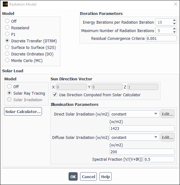
Controls
- Model
indicates which model, if any, is used to calculate radiation heat transfer. See Modeling Radiation for details about modeling radiation heat transfer.
- Off
disables the calculation of radiation heat transfer.
- Rosseland
enables the Rosseland radiation model.
- P1
enables the P-1 radiation model.
- Discrete Transfer (DTRM)
enables the discrete transfer radiation model (DTRM).
- Surface to Surface (S2S)
enables the surface-to-surface (S2S) radiation model.
- Discrete Ordinates (DO)
enables the discrete ordinates (DO) radiation model.
- Monte Carlo (MC)
enables the Monte Carlo (MC) radiation model.
- DO/Energy Coupling
allows you to couple the energy and DO intensity equations at each cell, solving them simultaneously. See Defining Non-Gray Radiation for the DO Model for details.
- Iteration Parameters
contains parameters related to the DTRM, S2S, and the DO models. This portion of the dialog box will appear only if Discrete Transfer (DTRM), Surface to Surface (S2S), or Discrete Ordinates (DO) is selected as the Model.
- Energy Iterations per Radiation Iteration
controls the frequency with which the radiation terms are updated as the continuous phase solution proceeds. The Energy Iterations per Radiation Iteration parameter is set to 10 by default. This implies that the radiation calculation is performed once every 10 iterations of the solution process. Increasing the number can speed the calculation process, but may slow overall convergence.
- Maximum Number of Radiation Iterations
controls the maximum number of iterations of the radiation calculation during each global iteration. The default setting of 5 means that the radiosity will be updated up to 5 times. The actual number of iterations will be less if the residual convergence criterion is exceeded at any point during these iterations.
This item appears only when Discrete Transfer or Surface to Surface is selected as the Model.
- Residual Convergence Criteria
determines when the radiation intensity update is converged. It is defined as the maximum normalized change in the surface intensity from one radiation iteration to the next (see Equation 16–4).
This item appears only when Discrete Transfer or Surface to Surface is selected as the Model.
- Target Number of Histories
determines the number of photon histories to be tracked for the Monte Carlo simulation. Too small of a number will produce "speckled" results. Increasing the target number of histories produces a smoother and more accurate solution, but at the expense of higher computation effort.
This item appears only when Monte Carlo is selected.
- View Factors and Clustering
contains parameters related to the S2S model. This portion of the dialog box will appear only if Surface to Surface is selected as the Model. See Setting Up the S2S Model for more information about the use of these parameters.
- Settings...
opens the View Factors and Clustering Dialog Box, in which you can set parameters related to surface clusters and view factors.
- Compute/Write/Read...
allows you to compute the view factors, write the computed view factors to a file, and read the file into Ansys Fluent. When you click Compute/Write/Read..., The Select File Dialog Box will open so that you can specify a name for the file where Ansys Fluent should save the view factors after computing them, and indicate whether the files should be saved in binary format.
- Read Existing File...
opens The Select File Dialog Box, in which you can specify the file from which Ansys Fluent should read view factors.
- Angular Discretization
contains parameters for angular discretization and pixelation for the DO model. This portion of the dialog box will appear only if Discrete Ordinates is selected as the Model. See Setting Up the DO Model for more information about the use of these parameters.
- Theta Divisions, Phi Divisions
define the number of control angles used to discretize each octant of the angular space (see Figure 5.3: Angular Coordinate System in the Theory Guide).
- Theta Pixels, Phi Pixels
are used to control the pixelation that accounts for any control volume overhang (see Figure 5.7: Pixelation of Control Angle in the Theory Guide and the figures and discussion preceding it).
- Radiation Mesh Options
This portion of the dialog box will appear only if the Monte Carlo model is selected.
- Target Cells Per Volume Cluster
Coarsens the radiation mesh used by the MC model. See Setting Up the MC Model for more information about the use of this parameter.
- Non-Gray Model
contains parameters related to the non-gray P-1, DO, or MC model. This portion of the dialog box will appear only if P1, Discrete Ordinates, or Monte Carlo is selected as the Model. See Setting Up the P-1 Model with Non-Gray Radiation, Defining Non-Gray Radiation for the DO Model, or Setting Up the MC Model for more information about the use of these parameters.
- Number of Bands
specifies the number of bands for the non-gray radiation.
- Wavelength Intervals (n=1)
contains inputs that define each wavelength band. (It appears only when the Number of Bands is nonzero.) For each band, you can specify a Name, as well as the Start and End wavelength of the band in
 m. Note that the wavelength bands are specified
for vacuum (
m. Note that the wavelength bands are specified
for vacuum ( ). Ansys Fluent will automatically
account for the refractive index in setting band limits for media
with
). Ansys Fluent will automatically
account for the refractive index in setting band limits for media
with  different from unity.
- Solar Load
contains parameters related to solar load model that can be used to calculate radiation effects from the sun’s rays that enter a computational domain. It is available only for the 3D version of Ansys Fluent. See Solar Load Model for more information about the use of these parameters.
- Model
indicates which model is used to calculate radiation effects.
- Off
disables the calculation of solar radiations.
- Solar Ray Tracing
enables the solar ray tracing algorithm
- DO Irradiation
enables the DO irradiation option. Select Discrete Ordinates under Model before selecting this option.
- Solar Calculator
opens the Solar Calculator Dialog Box.
- Sun Direction Vector
contains the components of sun direction vector.
- X, Y, Z
are the components of the sun direction vector.
- Use Direction Computed from Solar Calculator
enables the use of direction vector computed from the solar calculator.
- Illumination Parameters
contains illumination options.
- Direct Solar Irradiation
is the amount of energy per unit area due to direct solar irradiation.
- Diffuse Solar Irradiation
is the amount of energy per unit area due to diffuse solar irradiation.
- Spectral Fraction
is the fraction of incident solar radiation in the visible part of the solar radiation spectrum. The spectral fraction is not used for DO irradiation since the DO implementation is intended only for a single band. This parameter is available only for Solar Ray Tracing.
- Update Parameters
contains update parameters for transient simulations.
- Time Steps per Solar Load Update
specifies the number of time steps that will direct the Ansys Fluent solver to update the solar load data for the specified flow-time intervals in the unsteady solution process.
The View Factors and Clustering dialog box allows you to set parameters related to surface clusters and view factors for the surface-to-surface radiation model. See Setting Up the S2S Model for information about using this dialog box.
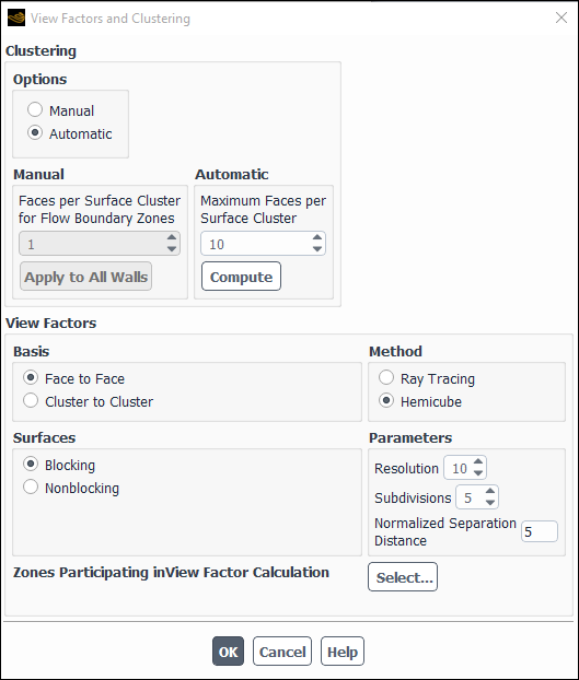
Controls
- Clustering
contains the methods and settings for creating surface clusters. See Forming Surface Clusters for information about surface cluster settings.
- Options
gives you a choice of forming clusters either manually or automatically.
- Manual
allows you to form clusters manually.
- Automatic
allows Ansys Fluent to form the cluster automatically.
- Manual
(available only when the Manual option is enabled) allows you to set the faces per surface cluster (FPSC) value for walls and inlet and outlet boundaries.
- Faces per Surface Cluster for Flow Boundary Zones
specifies the number of faces in each surface cluster for inlet and outlet boundaries (that is, exhaust fan, inlet vent, intake fan, outlet vent, mass-flow inlet, mass-flow outlet, pressure far-field, pressure inlet, pressure outlet, outflow, and velocity inlet boundaries). This FPSC value can also be applied to all walls that are adjacent to fluid zones by clicking the Apply to All Walls button. The default is set to
1. See Clustering in the Theory Guide for details about clustering.- Apply to All Walls
applies the value specified in the Faces per Surface Cluster for Flow Boundary Zones field to all walls that are adjacent to fluid zones.
- Automatic
(available only when the Automatic option is enabled) allows you to assign different faces per surface cluster (FPSC) values to the walls automatically, based on the distance of the walls from and the FPSC values of the walls that are defined as critical.
- Maximum Faces per Surface Cluster
specifies the maximum number of faces per surface cluster automatically assigned to non-critical wall zones adjacent to fluid zones. The default is set to
10.- Compute
results in Ansys Fluent automatically calculating and updating the face per surface cluster values in the boundary conditions dialog box for non-critical wall zones adjacent to fluid zones, without computing the clusters.
- View Factors
contains settings for computing the view factors. See Setting Up the View Factor Calculation for information about view factor calculation settings.
- Basis
specifies how surfaces are defined for the calculation of view factors. See Selecting the Basis for Computing View Factors for more information.
- Face to Face
specifies that the surfaces used to calculate the view factors are the boundary faces.
- Cluster to Cluster
specifies that the surfaces used to calculate the view factors are the clusters defined by the settings in the Clustering group box. The cluster to cluster basis is only available for 3D cases.
- Surfaces
specifies the geometric orientation of surface pairs with respect to each other when using the hemicube method.
- Blocking
specifies that the view factor calculation accounts for surfaces that block the views between the surfaces under consideration.
- Nonblocking
specifies that the view factor calculation does not account for surfaces that block the views between the surfaces under consideration.
- Method
specifies the method for computing the view factors. See Selecting the Method for Computing View Factors for information about choosing a method.
- Hemicube
specifies the use of the hemicube method for computing the view factors. The hemicube method is available only for 3D and axisymmetric cases, and should not be used if any of the zones are defined as periodic or symmetry boundaries.
- Ray Tracing
specifies the use of the ray tracing method for computing the view factors. For 2D cases, the number of rays used with this method is two times the value set for Resolution in the Parameters group box; for 3D cases, the number of rays is three times the square of the Resolution value.
- Parameters
contains settings related to the hemicube and ray tracing methods for computing the view factors. All of these inputs are available when Hemicube is selected under Method, whereas only Resolution is available when Ray Tracing is selected. See Selecting the Method for Computing View Factors for information about setting the method parameters.
- Resolution
specifies the resolution of the hemicube. The default value is set to
10. You can increase the value to reduce aliasing effects that can lead to overestimated or underestimated view factors.- Subdivisions
specifies the number of subfaces into which each face is divided. The default value is set to
5. This parameter is only available when the hemicube method is used in conjunction with the face to face basis.- Normalized Separation Distance
specifies the ratio of the minimum face separation to the effective diameter of the face. The default value is set to
5. This parameter is only available for the hemicube method.
- Zones Participating in View Factor Calculation
allows you to define which boundary zones participate in the view factor calculation. See Specifying Boundary Zone Participation for more information.
- Select...
opens the Participating Boundary Zones Dialog Box, where you can define which boundary zones participate in the view factor calculation.
The Participating Boundary Zones dialog box allows you to define which boundary zones participate in the view factor calculation, to display zones in the graphics window, and set the temperature of zones that do not participate in the view factor calculation. See Specifying Boundary Zone Participation for details. This dialog box opens when you click the Select... button next to the Zones Participating in View Factor Calculation label in the View Factors and Clustering dialog box.
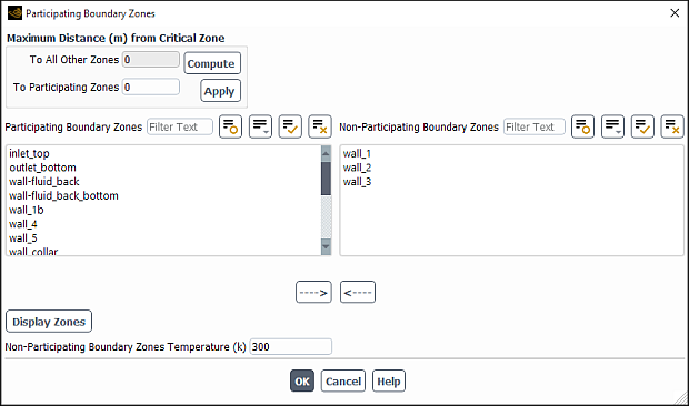
Controls
- Maximum Distance from Critical Zone
allows you to view the maximum distance between critical zones and other zones, and set all boundary zones that are located beyond a certain distance from a critical zone as not participating in the view factor calculation.
- To All Other Zones
displays the maximum of the distances between the centroids of critical and all other wall, inlet, and exit zones when the Compute button is clicked. This field is not editable. This is only available when using the Automatic option for clustering.
- Compute
calculates the distances between the centroids of critical zones and all the other wall, inlet, and exit zones and displays the maximum value in the To All Other Zones field and the To Participating Zones text-entry box. It requires the definition of the critical zone.
- To Participating Zones
displays the maximum of the distances between the centroids of critical and all other wall, inlet, and exit zones when the Compute button is clicked. Unlike the To All Other Zones field, you can edit this text-entry box. You can specify the maximum distance allowed between the centroids of critical zones and all other wall, inlet, or exit zones that participate in the view factor calculation; when you click the Apply button, all of the zones will be marked as either participating or not participating, according to the distance criteria you specified. Note that this field is only available when using the Automatic option for clustering.
- Apply
marks all of the wall, inlet, and exit zones as either participating or not participating in the view factor calculation, depending on whether the distance from their centroid to the centroid of a critical zone is equal to or less than value entered for To Participating Zones. The Participating Boundary Zones and Non-Participating Boundary Zones lists will be updated accordingly.
- Participating Boundary Zones
shows all the zones that are participating in the view factor calculation. You can select a zone and click the arrow button that points to the right to move the zone to the Non-Participating Boundary Zones list.
- Non-Participating Boundary Zones
shows all the zones that are not participating in the view factor calculation. You can select a zone and click the arrow button that points to the left to move the zone to the Participating Boundary Zones list.
- Display Zones
displays any zones selected in the Participating Boundary Zones and Non-Participating Boundary Zones lists in the graphics window.
- Non-Participating Boundary Zones Temperature
allows you to specify the temperature of the zones that do not participate in the view factor calculation.
The Solar Calculator dialog box allows you to set parameters related to the calculation of solar load models. See Solar Load Model for details. This dialog box opens when you click the Solar Calculator... button in the Radiation Model dialog box.
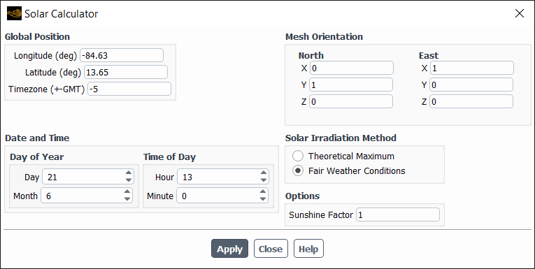
Controls
- Global Position
contains the parameters to define the position of solar radiation.
- Longitude
specifies the longitude of the desired location in degrees. Values may range from
 to
to  , where negative
values indicate the Western hemisphere and positive values indicate
the Eastern hemisphere.
, where negative
values indicate the Western hemisphere and positive values indicate
the Eastern hemisphere.- Latitude
specifies the latitude of the desired location in degrees. Values may range from
 (South pole) to
  (North pole) with
  defined as the equator.
- Timezone
specifies the local time zone of the desired location in hours relative to Greenwich Mean Time (+-GMT). This integer value can range from
 to
to  .
.
- Starting Date and Time
contains parameters to specify date and time.
- Day of Year
contains parameters to specify day and month.
- Time of Day
contains parameters to specify hour and minutes.
- Mesh Orientation
specifies the orientation as the vectors for North and East in the CFD grid system of coordinates.
- Solar Irradiation Method
contains parameters to choose the solar irradiation method.
- Theoretical Maximum
enables theoretically maximum solar irradiation method.
- Fair Weather Conditions
enables fair weather condition solar irradiation method.
- Sunshine Factor
is a linear reduction factor for the computed incident load that allows for cloud cover to be accounted for, if appropriate.
The Heat Exchanger Model dialog box allows you to define a heat exchanger as part of your model. See Modeling Heat Exchangers for details about using the items below.
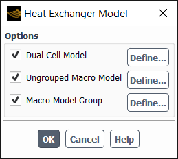
Controls
- Options
contains options related to the heat exchanger model. See Choosing a Heat Exchanger Model for details about the differences between the models associated with these options.
- Dual Cell Model
allows you to enable or disable the Dual Cell heat exchanger model. When this option is enabled, the corresponding Define... button opens the Dual Cell Heat Exchanger Dialog Box.
- Ungrouped Macro Model
allows you to enable or disable the Ungrouped Macro heat exchanger model. When this option is enabled, the corresponding Define... button opens the Ungrouped Macro Heat Exchanger Dialog Box.
- Macro Model Group
allows you to enable or disable the Macro heat exchanger group model. When this option is enabled, the corresponding Define... button opens the Macro Heat Exchanger Group Dialog Box.
The Dual Cell Heat Exchanger dialog box allows you to use the NTU method for heat transfer calculations. This model allows the solution of auxiliary flow on a separate mesh (other than the primary fluid mesh). See Using the Dual Cell Heat Exchanger Model for information about using this dialog box.
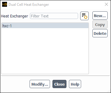
Controls
- Heat Exchanger
contains a list of predefined heat exchangers.
- New...
opens the Set Dual Cell Heat Exchanger Dialog Box.
- Copy
opens the Copy From Dialog Box, which allows you to copy the currently selected heat exchanger.
- Delete
removes the currently selected heat exchanger.
- Modify...
opens the Set Dual Cell Heat Exchanger Dialog Box.
The Set Dual Cell Heat Exchanger dialog box allows you to define the heat exchanger parameters. See Using the Dual Cell Heat Exchanger Model for details about using this dialog box.
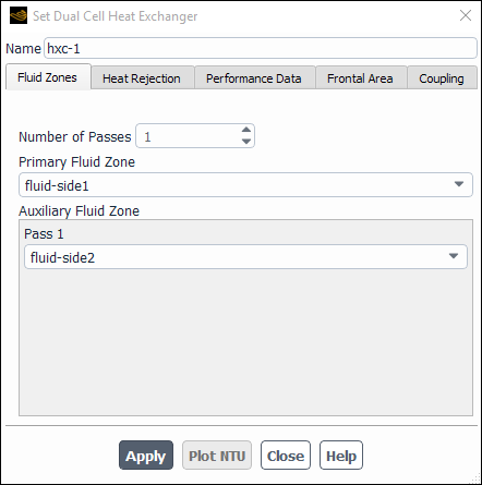
Controls
- Name
allows you to specify a name for the dual cell heat exchanger.
- Fluid Zones
allows you to specify the fluid zone parameters for the heat exchanger.
- Number of Passes
specifies the number of passes for the heat exchanger.
- Primary Fluid Zone
allows you to specify the fluid of the primary fluid zone for the heat exchanger.
- Auxiliary Fluid Zone
allows you to specify the fluid for the auxiliary fluid zone, per pass.
Important: The selected zones must be overlapping in physical space.
- Heat Rejection
contains parameters specific to the rejection of heat in the heat exchanger.
- Options
allows you to specify how the heat rejection in the heat exchanger is computed.
- Fixed Heat Rejection
allows you to specify heat rejection parameters.
- Fixed Inlet Temperature
allows you to use total heat rejection as the desired output.
- Heat Rejection Targeted
allows you to specify the heat rejection desired from the heat exchanger (available only when the Fixed Heat Rejection option is enabled).
- Inlet Zone for Temperature Updates
allows Ansys Fluent to change the temperature of the specified inlet zone in order to match the targeted heat rejection (available only when the Fixed Heat Rejection option is enabled).
- Temperature Update Under-Relaxation
controls convergence (available only when the Fixed Heat Rejection option is enabled).
- Iteration Interval Between Temperature Updates
controls divergence (available only when the Fixed Heat Rejection option is enabled).
- Performance Data
contains parameters for specifying the heat exchanger’s performance data.
- Options
allows you to choose between using raw performance data or NTU performance data.
- Raw Data
allows you to specify raw performance data for the heat exchanger.
- NTU Data
allows you to specify NTU performance data for the heat exchanger.
- Heat Exchanger Performance Data
contains parameters concerning the heat exchanger’s performance data.
- NTU Table
opens the NTU Table Dialog Box (available only when the NTU Data option is enabled).
- Heat Transfer Table
opens the Heat Transfer Data Table Dialog Box (available only when the Raw Data option is enabled).
- Effectiveness-NTU Relation
computes the NTU values from the heat transfer data. Choose cross-flow-unmixed, parallel-flow, or counter-flow, all of which are described in NTU Relations (available only when the Raw Data option is enabled).
- Reference Inlet Temperature
allows you to specify the inlet reference temperature for the primary and the auxiliary fluids. (Available only when the Raw Data option is enabled.)
- Frontal Area
allows you to specify the frontal area for the heat exchanger.
- Primary Fluid
allows you to specify a value for the Core Frontal Area for the primary fluid, or to compute the value from a surface zone using the Compute From drop-down list.
- Auxiliary Fluid
allows you to specify a value for the Core Frontal Area for the auxiliary fluid, or to compute the value from a surface zone using the Compute From drop-down list.
- Coupling
specifies parameters when you want to couple the heat exchanger passes.
- Temperature
specifies, by default, the mass-weighted average for the temperature of the outlet of Pass 1 to the inlet of Pass 2. Similarly, the mass-weighted-average temperature of the outlet of Pass 2 will be applied at the inlet zone of Pass 3, and so on. (Available only when multiple passes are specified in the Fluid Zones tab.)
- Plot NTU
plots the performance data curve for the selected heat exchanger. The performance data is supplied through the Performance Data tab.
The Heat Transfer Data Table dialog box contains information on the number of fluid flow rates and heat transfer data for the primary and auxiliary fluids. See Using the Ungrouped Macro Heat Exchanger Model for details about using this dialog box.
Controls
- Number of Auxiliary Fluid Flow Rates
sets the number of auxiliary fluid flow rates.
- Number of Primary Fluid Flow Rates
sets the number of primary fluid flow rates.
- Auxiliary Fluid Flow Rate
sets fluid flow rates for the auxiliary fluid.
- Primary Fluid Flow Rate
sets fluid flow rates for the primary fluid.
- Heat Transfer
sets the heat transfer for the corresponding primary and auxiliary fluid flow rates.
- Read...
allows you to read in a file containing heat transfer data.
- Write...
allows you to write a file containing heat transfer data.
The NTU Table dialog box contains information on the number of fluid flow rates and NTU data for the primary and auxiliary fluids. See Using the Ungrouped Macro Heat Exchanger Model for details about using this dialog box.
Controls
- Number of Auxiliary Fluid Flow Rates
sets the number of auxiliary fluid flow rates.
- Number of Primary Fluid Flow Rates
sets the number of primary fluid flow rates.
- Auxiliary Fluid Flow Rate
sets fluid flow rates for the auxiliary fluid.
- Primary Fluid Flow Rate
sets fluid flow rates for the primary fluid.
- NTU
sets the NTU values for the corresponding primary and auxiliary fluid flow rates.
- Read...
allows you to read in a file containing NTU data.
- Write...
allows you to write a file containing NTU data.
The Copy From dialog box allows you to copy the setup of one heat exchanger to another.
Controls
- Existing Heat Exchangers
contains a list of heat exchangers, from which you can copy the settings from one heat exchanger to another.
The Ungrouped Macro Heat Exchanger dialog box allows you to set up the ungrouped macro heat exchanger model. See Using the Ungrouped Macro Heat Exchanger Model for details about using this dialog box.
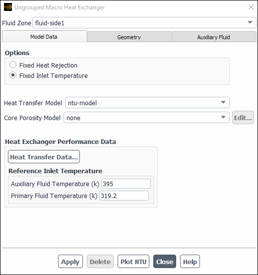
Controls
- Fluid Zone
specifies the zone that represents the heat exchanger.
- Model Data
contains the parameters related to the heat exchanger model.
- Options
allows you to choose one of the following settings:
- Fixed Heat Rejection
specifies that Ansys Fluent should compute the auxiliary fluid inlet temperature for a specified heat rejection.
- Fixed Inlet Temperature
specifies that Ansys Fluent should compute the total heat rejection of the core for a given inlet auxiliary temperature.
- Heat Transfer Model
allows you to specify either the ntu-model or the simple-effectiveness-model for heat transfer. See Choosing a Heat Exchanger Model for information on the differences between these models.
- Core Porosity Model
contains a drop-down list of all available core porosity models.
- Edit...
opens the Core Porosity Model Dialog Box.
- Heat Exchanger Performance Data
contains the parameters for heat transfer.
- Heat Transfer Data...
opens the Heat Transfer Data Table Dialog Box. This item will appear for the NTU model only.
- Auxiliary Fluid Temperature
specifies the auxiliary fluid temperature. This item will appear only for the NTU model.
- Primary Fluid Temperature
specifies the gas stream temperature. This item will appear only for the NTU model.
- Velocity Effectiveness Curve...
opens the Velocity Effectiveness Curve Dialog Box in which you can define the effectiveness of the heat exchanger core (
 in Equation 6–11 in the Theory Guide). This
item will appear for simple effectiveness model only.
in Equation 6–11 in the Theory Guide). This
item will appear for simple effectiveness model only.
- Geometry
contains parameters to define the macro grid.
- Width
sets the width of the heat exchanger core. The Width is measured in the pass-to-pass direction.
- Height
sets the height of the heat exchanger core. The Height is measured in the auxiliary fluid inlet direction.
- Depth
sets the depth of the heat exchanger core.
- Number of Passes
specifies the number of passes for the macro grid. (See Figure 16.76: 1x4x3 Macros.)
- Number of Rows/Pass, Number of Columns/Pass
specify the number of macro rows and columns per pass in the macro grid. (See Figure 16.76: 1x4x3 Macros.)
- View Passes
displays the macro grid. (This button becomes available after you click Apply.) The path of the auxiliary fluid is color-coded in the display: macro
 is red and macro
  is blue.
- Draw Mesh
toggles between displaying and not displaying the mesh when the macro mesh is displayed (using the View Passes button). The Mesh Display Dialog Box opens when Draw Mesh is selected.
- Update from Plane Tool
updates the Auxiliary Fluid Inlet Direction and Pass-to-Pass Direction from the plane tool orientation. The Width, Height, and Depth will also be updated. See Using the Plane Tool for information about using the plane tool.
Open the Plane Surface Dialog Box to make the plane tool appear.
- Auxiliary Fluid Inlet Direction (height)
specifies the direction in which the auxiliary fluid enters the heat exchanger. See Figure 16.76: 1x4x3 Macros.
- Pass-to-Pass Direction (width)
specifies the direction in which the auxiliary fluid moves at the end of each pass through the heat exchanger. See Figure 16.76: 1x4x3 Macros.
- Auxiliary Fluid
contains the option to specify the auxiliary fluid properties.
- Auxiliary Fluid Properties Method
contains options for specifying auxiliary fluid properties.
- constant-specific-heat
allows you to specific a constant value for the auxiliary fluid specific heat.
- user-defined-enthalpy
allows you to specify a user-defined function for the auxiliary fluid enthalpy.
- Auxiliary Fluid Specific Heat
specifies the value of
 in Equation 6–17 in the Theory Guide. This value is specified only
if constant-specific-heat is selected.
in Equation 6–17 in the Theory Guide. This value is specified only
if constant-specific-heat is selected.- Auxiliary Fluid Enthalpy UDF
allows you to specify a user-defined function for the auxiliary fluid enthalpy (see Equation 6–17 in the Theory Guide). This option is available only when user-defined-enthalpy is selected.
- Auxiliary Fluid Flow Rate
sets the flow rate of the auxiliary fluid (
 in Equation 6–16 in the Theory Guide).
- Heat Rejection
sets the total heat rejection (
 in Equation 6–15 in the Theory Guide). This
value is specified only if Fixed Heat Rejection is selected.
in Equation 6–15 in the Theory Guide). This
value is specified only if Fixed Heat Rejection is selected.- Initial Temperature
sets an initial guess for the inlet temperature (
 in Equation 6–11 and Equation 6–16 in the Theory Guide). This value is specified
only if Fixed Heat Rejection is selected.
in Equation 6–11 and Equation 6–16 in the Theory Guide). This value is specified
only if Fixed Heat Rejection is selected.- Inlet Temperature
sets the auxiliary fluid initial temperature (
 in Equation 6–11 and Equation 6–16 in the Theory Guide). This
value is specified only if Fixed Inlet Temperature is selected in the Model Data tab.
in Equation 6–11 and Equation 6–16 in the Theory Guide). This
value is specified only if Fixed Inlet Temperature is selected in the Model Data tab.- Inlet Pressure
sets the auxiliary fluid inlet pressure. This value is specified only if user-defined-enthalpy is selected.
- Inlet Quality
specifies the value of
 in Equation 6–20 in the Theory Guide. This value is specified only
if user-defined-enthalpy is selected.
in Equation 6–20 in the Theory Guide. This value is specified only
if user-defined-enthalpy is selected.- Pressure Drop
specifies the value of
 in Equation 6–21 in the Theory Guide. This value
is specified only if user-defined-enthalpy is
selected.
in Equation 6–21 in the Theory Guide. This value
is specified only if user-defined-enthalpy is
selected.
- Apply
saves all the settings for the heat exchanger specified in the Fluid Zone list.
- Delete
deletes the heat exchanger specified in the Fluid Zone list.
The Velocity Effectiveness Curve dialog box allows you to define effectiveness curve. It is opened by clicking Velocity Effectiveness Curve... in the Ungrouped Macro Heat Exchanger Dialog Box.
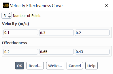
Controls
- Number of Points
specifies the number of data pairs in the effectiveness profile. The default value of 1 indicates a constant effectiveness.
- Velocity, Effectiveness
specify the data pairs for the effectiveness profile. These items are available only if the simple effective model has been selected. Note that the Effectiveness values must be within the range of 0–1.
The Core Porosity Model dialog box allows you to modify or define a heat exchanger core model. This dialog box opens when you click Edit... in the Ungrouped Macro Heat Exchanger Dialog Box.
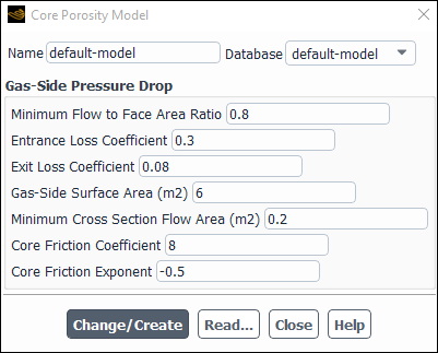
Controls
- Name
specifies the name of a new heat exchanger core model.
- Database
contains a drop-down list of all heat exchanger core models that are currently available.
- Gas-Side Pressure Drop
contains parameters that define the air-side pressure drop.
- Minimum Flow to Face Area Ratio
sets the value of
 in Equation 6–2 in the Theory Guide.
- Entrance Loss Coefficient
sets the value of
 in Equation 6–2 in the Theory Guide.
- Exit Loss Coefficient
sets the value of
 in Equation 6–2 in the Theory Guide.
- Gas Side Surface Area
sets the value of
 in Equation 6–2 in the Theory
Guide.
in Equation 6–2 in the Theory
Guide.- Minimum Cross Section Flow Area
sets the value of
 in Equation 6–2 in the Theory Guide.
- Core Friction Coefficient
sets the value of
 in Equation 6–3 in the Theory Guide.
- Core Friction Exponent
sets the value of
 in Equation 6–3 in the Theory Guide.
- Change/Create
saves the settings in the dialog box and adds the new model to the Database list.
- Read...
opens The Select File Dialog Box, in which you can select an external file containing a predefined heat exchanger core model.
The Macro Heat Exchanger Group dialog box allows you to modify or define a heat exchanger core group.
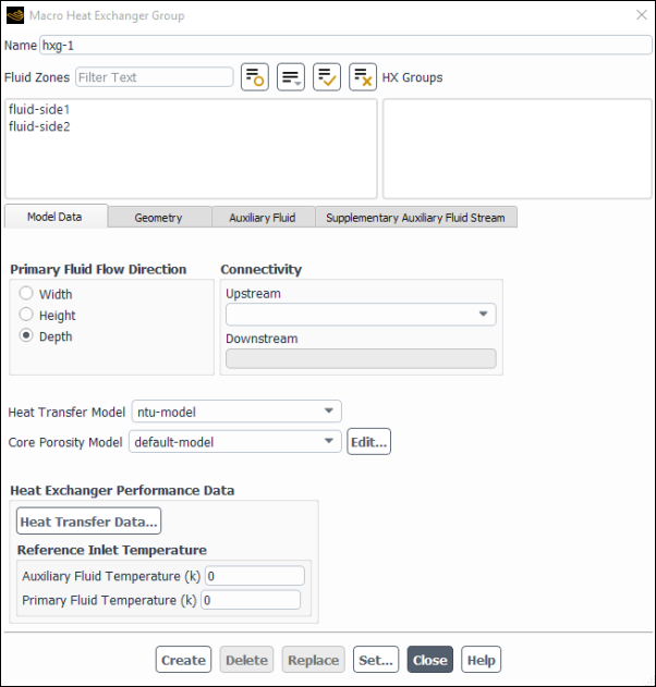
Controls
- Name
specifies the name of a new heat exchanger group.
- Fluid Zones
contains a list of all the fluid zones.
- HX Groups
contains list of the heat exchanger groups.
- Model Data
contains all the parameters to be specified for the model.
- Primary Fluid Flow Direction
gives you a choice of gas flow direction.
- Width, Height, Depth
specifies the width, height and the depth of the gas flow direction.
- Connectivity
allows you to define the upstream and downstream connections.
- Upstream
specifies the upstream heat exchanger group.
- Downstream
specifies the downstream heat exchanger group.
- Heat Transfer Model
allows you to select either the simple-effectiveness-model or the ntu-model. See Choosing a Heat Exchanger Model for information on the differences between these models.
- Core Porosity Model
specifies whether default values are chosen for the core porosity model.
- Edit...
opens the Core Porosity Model Dialog Box for the definition of a new core porosity model.
- Heat Exchanger Performance Data
contains the parameters for heat transfer.
- Heat Transfer Data...
opens the Heat Transfer Data Table Dialog Box. This dialog box allows you to define the heat transfer for different primary and auxiliary fluid flow rates. This item will appear for the NTU model only.
- Velocity Effectiveness Curve...
opens the Velocity Effectiveness Curve Dialog Box in which you can define the effectiveness of the heat exchanger core (
 in Equation 6–11 in the Theory Guide). This
item will appear for simple effectiveness model only.
in Equation 6–11 in the Theory Guide). This
item will appear for simple effectiveness model only.- Auxiliary Fluid Temperature
specifies the auxiliary fluid temperature. This item will appear for the NTU model only.
- Primary Fluid Temperature
specifies the gas stream fluid temperature. This item will appear for the NTU model only.
- Geometry
contains parameters to define the macro grid.
- Width, Height, Depth
specifies the width, height and the depth of the heat exchanger.
- Number of Passes
specifies the number of passes.
- Number of Rows/Pass
specifies the number of rows per pass.
- Number of Columns/Pass
specifies the number of columns per pass.
- View Passes
displays the macro grid. (This button becomes available after you click Set.) The path of the auxiliary fluid is color-coded in the display: macro
 is red and macro
  is blue.
- Draw Mesh
toggles between displaying and not displaying the mesh when the macro mesh is displayed (using the View Passes button). The Mesh Display Dialog Box opens when Draw Mesh is selected.
- Update from Plane Tool
updates the Auxiliary Fluid Inlet Direction and Pass-to-Pass Direction from the plane tool orientation. The Width, Height, and Depth will also be updated. See Using the Plane Tool for information about using the plane tool.
- Auxiliary Fluid Inlet Direction
specifies the direction in which the auxiliary fluid enters the heat exchanger. See Figure 16.76: 1x4x3 Macros.
- Pass-to-Pass Direction
specifies the direction in which the auxiliary fluid moves at the end of each pass through the heat exchanger. See Figure 16.76: 1x4x3 Macros.
- Auxiliary Fluid
contains inputs to specify the properties of the auxiliary fluid.
- Properties Method
specifies the method to specify the auxiliary fluid properties. You can choose from constant-specific-heat and user-defined-enthalpy.
- Specific Heat
sets the specific heat of the auxiliary fluid (
 in Equation 6–16 you choose constant-specific-heat.
- Enthalpy UDF
sets the enthalpy as defined by the user-defined function selected from the drop-down list.
- Auxiliary Fluid Flow Rate
sets the flow rate of the auxiliary fluid (
 in Equation 6–16 in the Theory Guide).
- Initial Temperature
sets an initial guess for the inlet temperature (
 in Equation 6–11 and Equation 6–16 in the Theory Guide). This value is specified
only if Fixed Heat Rejection is selected.
in Equation 6–11 and Equation 6–16 in the Theory Guide). This value is specified
only if Fixed Heat Rejection is selected.- Inlet Pressure
sets the auxiliary fluid inlet pressure. This value is specified only if user-defined-enthalpy is selected.
- Inlet Quality
specifies the value of
 in Equation 6–20 in the Theory Guide.
- Pressure Drop
specifies the value of
 in Equation 6–21 in the Theory Guide. This value
is specified only if user-defined-enthalpy is
selected.
in Equation 6–21 in the Theory Guide. This value
is specified only if user-defined-enthalpy is
selected.
- Supplementary Auxiliary Fluid Stream
specifies properties of the supplementary auxiliary stream.
- Supplementary Mass Flow Rate
specifies the supplementary fluid flow rate as constant, polynomial or piecewise-linear.
- Supplementary Flow Temperature
specifies the supplementary fluid temperature as constant, polynomial or piecewise-linear.
- Supplementary Flow Quality
specifies the supplementary fluid quality.
- Create
saves all the settings in the dialog box.
- Delete
deletes the group that is selected in the HX Groups list.
- Replace
changes the parameters of the already existing group that is selected in the HX Groups list.
- Set...
opens the Ungrouped Macro Heat Exchanger Dialog Box, in which you can define a new heat exchanger core model or read one from an external file.
Important: This feature offers reduced functionality when running Fluent under the Pro capability level.
The Species Model dialog box allows you to set parameters related to the calculation of species transport and combustion. For details about the items below, see the following sections:
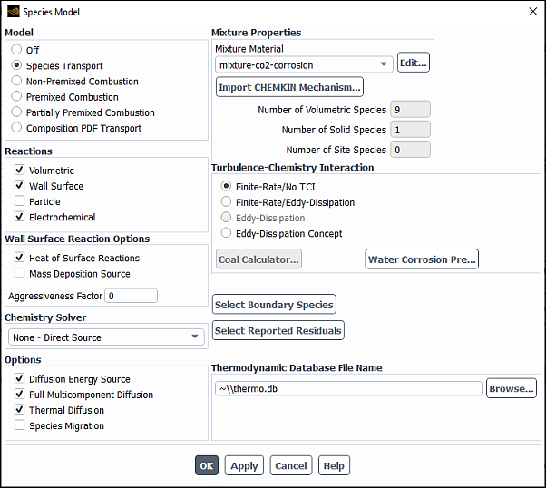
Controls
- Model
indicates which model, if any, is used to calculate species transport/combustion.
- Off
disables species calculations.
- Species Transport
enables the calculation of multi-species transport (either non-reacting or reacting, depending on the selection for Reactions). See Modeling Species Transport and Finite-Rate Chemistry for details.
- Non-Premixed Combustion
enables the calculation of turbulent reacting flow using the non-premixed combustion model. See Modeling Non-Premixed Combustion for details. This option is available only for turbulent flows using the pressure-based solver.
- Premixed Combustion
enables the premixed turbulent combustion model. See Modeling Premixed Combustion for details. This option is available only for turbulent flows using the pressure-based solver.
- Partially Premixed Combustion
enables the partially premixed turbulent combustion model. See Modeling Partially Premixed Combustion for details. This option is available only for turbulent flows using the pressure-based solver.
- Composition PDF Transport
enables the composition PDF transport model. See Modeling a Composition PDF Transport Problem for details. This option is available only for turbulent flows using the pressure-based solver.
- Reactions
contains options related to the modeling of reacting flow. (This section of the dialog box appears only when Species Transport or Composition PDF Transport is the specified Model.)
- Volumetric
enables the calculation of reacting flow using the finite-rate formulation. See Volumetric Reactions for details.
- Wall Surface
enables the calculation of wall surface reactions. See Wall Surface Reactions and Chemical Vapor Deposition for details. This item will appear only if Volumetric is enabled.
- Particle
enables the calculation of particle reactions. See Particle Reactions for details. This item will appear only if Volumetric is enabled.
- Electrochemical
enables the calculation of electrochemical reactions. See Electrochemical Reactions for details. This item will appear only if Volumetric is enabled.
- Integration Parameters...
is a command button that opens the Integration Parameters Dialog Box. This button appears for the species transport model, when Volumetric is enabled under Reactions and Stiff Chemistry Solver is enabled under Options or when Eddy-Dissipation Concept is enabled under Turbulence-Chemistry Interaction.
- Wall Surface Reaction Options
contains additional options for wall surface reactions. This portion of the dialog box appears only if Wall Surface is enabled under Reactions.
- Heat of Surface Reactions
(if enabled) includes the heat release due to surface reactions in the energy equation. You must remember to set appropriate formation enthalpies (standard state enthalpies) if you enable this option.
- Mass Deposition Source
when enabled, includes the effect of surface mass transfer in the continuity equation. This option is always enabled when the density-based solver is used. With the density-based solver, the effect of surface mass transfer in the continuity equation is always included.
- Aggressiveness Factor
is a numerical factor that controls the robustness and the convergence speed. This value ranges between 0 and 1, where 0 is the most robust, but results in the slowest convergence. The default value for the Aggressiveness Factor is 0.5. This parameter appears only when the pressure-based solver is used.
- Chemistry Solver
is a drop-down list in which you can select the solver for the chemically reactive flow simulation. This item appears only for Species Transport and Composition PDF Transport models involving Volumetric reactions.
- Stiff Chemistry Solver
enables efficient integration of stiff chemical kinetics. This item appears only when Finite-Rate/No TCI or Eddy-Dissipation Concept is selected in the Turbulence-Chemistry Interaction group box. See Solution of Stiff Chemistry Systems for details.
- CHEMKIN-CFD Solver
enables the integration of chemical kinetics using the Ansys CHEMKIN-CFD Solver, designed for large, stiff chemistry mechanisms. This item appears only when Finite-Rate/No TCI or Eddy-Dissipation Concept is selected in the Turbulence-Chemistry Interaction group box.
- Relax to Chemical Equilibrium
enables efficient modeling of chemical kinetics effects based only on equilibrium calculation and assumptions about characteristic timescales for approaching equilibrium. This item is not available for the Eddy Dissipation Concept TCI option. (See The Relaxation to Chemical Equilibrium Model for details.
- None - Direct Source
makes explicit use of chemistry source terms in the species transport equations, without a stiff-chemistry solver (not recommended for stiff or complex chemistry).
- Options
contains additional options for the Species Transport and Composition PDF Transport models only. This group box will not appear in the dialog box for the other models.
- Diffusion Energy Source
(if enabled) includes the effect of enthalpy transport due to species diffusion in the energy equation.
- Full Multicomponent Diffusion
enables the full multicomponent diffusion model. See Full Multicomponent Diffusion in the Fluent Theory Guide for details.
- Thermal Diffusion
enables the thermal diffusion model. See Thermal Diffusion Coefficients in the Fluent Theory Guide for details.
- Liquid Micro-Mixing
is used to model liquid reactions. When the Liquid Micro-Mixing model is invoked, Ansys Fluent uses the volume-weighted-mixing-law formula to calculate the density.
- Species Migration
(if enabled) includes the ion species migration term in the species transport equation. This item appears only when Electrochemical reactions are enabled.
- Thickened Flame Model
enables the modeling of laminar flames. This application is typically used as an LES combustion model for turbulent premixed and partially-premixed flames.
- Include Temperature Fluctuations
enables the calculation of the multi-mode energy equation. This option is available when the composition PDF transport model is selected.
- Mixture Properties
contains controls and information about the mixture being modeled. This section of the dialog box will not appear if Premixed Combustion is the selected under Model.
- Mixture Material
contains a drop-down list of available mixture materials. When you first enable the Species Transport model, you can choose from all of the mixture materials defined in the database, or you can choose a "template" and define your own material. (Click View... to open the Fluent Database Materials Dialog Box and check the properties of the mixture material selected in the list.) See Enabling Species Transport and Reactions and Choosing the Mixture Material for details.
When you use the Non-Premixed Combustion or Partially Premixed Combustion model, this list will be inactive. The mixture material for a non-premixed or partially premixed combustion calculation will be determined from the content of the PDF file generated in Ansys Fluent using the PDF Options parameters.
- Number of Volumetric Species
specifies the number of gas-phase species in the selected Mixture Material. This is an informational display only; you cannot edit this value.
- Number of Solid Species
specifies the number of solid species defined in the selected Mixture Material. This is an informational display only; you cannot edit this value. (This list will appear only for Species Transport models involving Wall Surface reactions.)
- Number of Site Species
specifies the number of site species defined in the selected Mixture Material. This is an informational display only; you cannot edit this value. (This list will appear only for Species Transport models involving Wall Surface reactions.)
- Turbulence-Chemistry Interaction
indicates which model is to be used for turbulence-chemistry interaction when the Species Transport model with Volumetric reactions is used.
- Finite-Rate/No TCI
computes only the Arrhenius rate (see Equation 7–21 in the Theory Guide) and neglects turbulence-chemistry interaction.
- Finite-Rate/Eddy-Dissipation
(for turbulent flows) computes both the Arrhenius rate and the mixing rate and uses the smaller of the two.
- Eddy-Dissipation
(for turbulent flows) computes only the mixing rate (see Equation 7–39 and Equation 7–40 in the Theory Guide).
- Eddy-Dissipation Concept
(for turbulent flows) models turbulence-chemistry interaction with detailed chemical mechanisms (see Equation 7–39 and Equation 7–40 in the Theory Guide).
- Coal Calculator...
opens the Coal Calculator Dialog Box.
- Water Corrosion Pre...
opens the dialog box. This item is available only for the Species Transport model with electrochemical reactions. See Procedure for Setting Corrosion Simulations using the Water Corrosion Pre Tool for additional information on using the dialog box.
- Select Boundary Species...
opens the Select Boundary Species dialog box (see Figure 19.3: The Select Boundary Species Dialog Box).
- Select Reported Residuals
opens the Select Residual Monitored Species dialog box (see Figure 19.4: The Select Residual Monitored Species).
- Options
contains parameters related to the laminar finite-rate or the eddy-dissipation concept model. This section of the dialog box will appear when Finite-Rate/No TCI or the Eddy-Dissipation Concept is selected for Turbulence-Chemistry Interaction.
- EDC Model
(Eddy-Dissipation Concept only) contains the following submodels:
Constant Coefficients (default): Standard EDC model (see The Standard EDC Model in the Fluent Theory Guide for details)
Partially Stirred Reactor: Partially stirred reactor EDC model (see The Partially Stirred Reactor EDC Model in the Fluent Theory Guide for details)
- Flow Iterations Per Chemistry Update
(steady-state only) specifies how often Ansys Fluent will update the chemistry during the calculation. Increasing the number can reduce the computational expense of the chemistry calculations. This option is not available when the None - Direct Source option is selected for Chemistry Solver.
- Aggressiveness Factor
(steady-state only) is a numerical factor that controls the robustness and the convergence speed. This value ranges between 0 and 1, where 0 is the most robust, but results in the slowest convergence. The default value for the Aggressiveness Factor is 0.5. This option is available only when Stiff Chemistry Solver or CHEMKIN CFD Solver is selected for Chemistry Solver.
- Temperature Threshold
is the threshold for cell temperature below which the chemistry reaction rate in the cell will be set to zero. This may improve the computational time without sacrificing accuracy. The default value is 200 K. This option is available only when Stiff Chemistry Solver or CHEMKIN CFD Solver is selected for Chemistry Solver.
- Volume Fraction Constant
specifies the value of
 in Equation 7–44 in the
Theory Guide. This item appears only
for the Constant Coefficients EDC model.
in Equation 7–44 in the
Theory Guide. This item appears only
for the Constant Coefficients EDC model.- Time Scale Constant
specifies the value of
 in Equation 7–45 in the
Theory Guide. This item appears only
for the Constant Coefficients EDC model.
in Equation 7–45 in the
Theory Guide. This item appears only
for the Constant Coefficients EDC model.- Mixing Model
(Partially Stirred Reactor EDC model only) is a group box where you can select how
 in Equation 7–50 in the Fluent Theory Guide is
computed:
in Equation 7–50 in the Fluent Theory Guide is
computed:Constant Cmix: Sets
 to a constant value specified in Mixing Constant
Dynamic Cmix (default): Computes
 by Equation 7–51 in the Fluent Theory Guide
with the fractal dimension
by Equation 7–51 in the Fluent Theory Guide
with the fractal dimension  in Equation 7–52 in the Fluent Theory Guide
specified in Fractal Dimension
in Equation 7–52 in the Fluent Theory Guide
specified in Fractal Dimension
- Thickened Flame Model Options
contains parameters related to the thickened flame model. This group box is displayed only if the Thickened Flame Model is enabled in the Options group box.
- Efficiency Function
allows you to select the efficiency function. You can choose between none, Colin (default), or Charlette. See The Thickened Flame Model in the Fluent Theory Guide for more information about these options.
- Number of Grid Points in Flame
by default are 8 grid points.
- Integral Length Scale
is the representative of the largest eddy sizes,
 in Equation 7–57 in the Fluent Theory Guide
(typically, 1/4 to 1/2 of a characteristics dimension, such as a burner diameter, an inlet
diameter, or a size of a bluff body). This item is available only for simulations with the
Large Eddy Simulation (LES) turbulence model when Colin is used as the
efficiency function.
in Equation 7–57 in the Fluent Theory Guide
(typically, 1/4 to 1/2 of a characteristics dimension, such as a burner diameter, an inlet
diameter, or a size of a bluff body). This item is available only for simulations with the
Large Eddy Simulation (LES) turbulence model when Colin is used as the
efficiency function.
- PDF Options
contains options related for the non-premixed combustion model. (This section will appear only if Non-Premixed Combustion or Partially-Premixed Combustion is the selected Model.)
- Inlet Diffusion
includes the diffusion flux of species at inlet.
- Compressibility Effects
can be enabled to account for cases where substantial pressure changes occur in time and/or space when modeling a non-adiabatic system. See Specifying the Operating Pressure for the System for details.
- Liquid Micro-Mixing
is used to model liquid reactions. When the Liquid Micro-Mixing model is invoked, Ansys Fluent uses the volume-weighted-mixing-law formula to calculate the density.
- Probability Density Function
is a drop-down list that allows you to choose between the shape of the assumed probability density function (PDF):
double delta: as given by Equation 8–21 in the Fluent Theory Guide.
beta: as given by Equation 8–22 in the Fluent Theory Guide.
This control appears after you generate or read a PDF table into Ansys Fluent.
- Chemistry
tab contains the parameters to define problems using the chemistry model. See Setting Up the Equilibrium Chemistry Model for details.
- State Relation
- Chemical Equilibrium
enables the equilibrium chemistry model. See Setting Up the Equilibrium Chemistry Model for details.
- Steady Diffusion Flamelet
enables the steady diffusion flamelet model. See The Diffusion Flamelet Models Theory in the Theory Guide for details.
- Unsteady Diffusion Flamelet
enables the Eulerian unsteady diffusion flamelet model.
- Diesel Unsteady Flamelet
enables the diesel unsteady laminar flamelet model. See Using the Diesel Unsteady Laminar Flamelet Model for details.
- Flamelet Generated Manifold
enables the flamelet generated manifold (FGM) model. This is available when the Partially Premixed Combustion model is selected. See Partially Premixed Combustion in the Theory Guide for details.
- Energy Treatment
- Adiabatic
enables adiabatic modeling options for the problem.
- Non-Adiabatic
enables non-adiabatic modeling options for the problem. See Non-Adiabatic Extensions of the Non-Premixed Model in the Theory Guide for details.
- Coal Calculator
opens the Coal Calculator Dialog Box.
- Stream Options
contains the parameters for the equilibrium chemistry model or the steady diffusion flamelet model.
- Secondary Stream
includes the secondary inlet stream in the model.
- Empirical Fuel Stream
enables parameters to define fuel stream empirically. This option is available only with the full equilibrium chemistry model.
- Empirical Secondary Stream
enables parameters to define secondary stream empirically. This option is available only with the full equilibrium chemistry model.
- Model Settings
contains a list of parameter settings.
- Operating Pressure
specifies the system operating pressure used to calculate the density using the ideal gas law. See Specifying the Operating Pressure for the System for details.
- Fuel Stream Rich Flammability Limit
specifies the rich flammability limit for fuel stream when the equilibrium chemistry option is used. You will not set these if you have used the empirical definition option for fuel composition. See Enabling the Rich Flammability Limit (RFL) Option for details.
- Secondary Stream Flammability Limit
specifies the rich flammability limit for secondary stream when the equilibrium chemistry option is used. You will not set these if you have used the empirical definition option for fuel composition. See Enabling the Rich Flammability Limit (RFL) Option for details.
- Empirical Fuel Lower Calorific Value
specifies the lower calorific value of fuel stream.
- Empirical Fuel Specific Heat
specifies the specific heat value of fuel stream.
- Empirical Fuel Molecular Weight
specifies the molecular weight of the fuel stream.
- Empirical Secondary Lower Calorific Value
specifies the lower calorific value of secondary stream.
- Empirical Secondary Specific Heat
specifies the specific heat value of secondary stream.
- Empirical Secondary Molecular Weight
specifies the molecular weight of the secondary stream.
- Options
contains options related to the steady flamelet model.
- Create Flamelet
enables the Import CHEMKIN Mechanism... button that opens the Import CHEMKIN Format Mechanism Dialog Box where you can import the CHEMKIN mechanism and thermodynamic data, to create a flamelet file. This option is available for the steady flamelet model. See Setting Up the Steady and Unsteady Diffusion Flamelet Models for details.
- Import Flamelet
enables the Import Flamelet File... button that opens The Select File Dialog Box where you can select the existing flamelet in Ansys Fluent. You can also set the file type parameters to import the existing flamelet in Ansys Fluent. See Setting Up the Steady and Unsteady Diffusion Flamelet Models for details. This option is available for the steady flamelet model.
- Flamelet Type
gives you the option of creating a Premixed Flamelet or a Diffusion Flamelet. This is available when the Flamelet Generated Manifold model is selected.
- Flamelet Solution Method
allows you to solve the premixed FGM either in the CHEMKIN Physical Space or in the Progress Variable Space. This is available when the Flamelet Generated Manifold state reaction is selected and Premixed Flamelet is selected as the Flamelet Type.
- File Type
contains the toggle buttons for two flamelet file types.
- Standard
enables the import of an ASCII format standard flamelet file.
- CFX-RIF
enables the import of an ASCII format CFX-RIF flamelet file.
- Flamelet Property File Name
opens The Select File Dialog Box in which you can save the existing flamelet in Ansys Fluent to use when running an existing case.
- Thermodynamic Database File Name
specifies a path for the thermodynamic database file to be read.
- Boundary
tab contains the list of boundary species and related parameters. See Defining the Stream Compositions for details.
- Species
contains the list of the species used in the problem.
- Fuel
specifies the fuel species.
- Oxid
specifies the oxidizing species.
- Second
specifies the secondary species.
- Boundary Species
allows you to specify the species you want to add or remove from the model. You can type the species chemical formula in the field below it.
- Add
adds the species in the model.
- Remove
removes the species from the model.
- List Available Species
prints a list of all species in the thermodynamic database file (
thermo.db) in the console window.
- Temperature
specifies the temperature of different streams that you have defined.
- Fuel
is the temperature of the fuel inlet in the model.
- Oxid
is the temperature of the oxidizer inlet in the model.
- Second
is the temperature of the secondary stream inlet in the model.
- Specify Species in
allows you to define the unit of species concentration.
- Mass Fraction
allows you to specify the species in terms of mass fraction.
- Mole Fraction
allows you to specify the species in terms of mole fraction.
- Control
tab contains the parameters for exclusion and inclusion of equilibrium species. This is available only for equilibrium chemistry model. See Forcing the Exclusion and Inclusion of Equilibrium Species for details.
- Species Excluded from Equilibrium
lists the species excluded from equilibrium calculation.
- Species
lists the slow-forming species that are zeroed in the initial flamelet profile.
- Add
allows you to add equilibrium species.
- Remove
allows you to remove equilibrium species.
- List Available Species
prints a list of all species in the thermodynamic database file in the console window.
- Flamelet Controls
allows you to adjust the controls for the flamelet solution. Note that the Create Flamelet option in the Chemistry tab must be selected for the Steady Diffusion Flamelet or Flamelet Generated Manifold models for these controls to be available.
- Initial Fourier Number
sets the size for the first time step for the solution.
- Fourier Number Multiplier
increases the time step size at subsequent times. The size for every time step after the first is multiplied by this value.
- Relative Error Tolerance and Absolute Error Tolerance
specifies the local error controls during numerical integration.
- Flamelet Convergence Tolerance
specifies the maximum absolute change in species fraction or temperature at any discrete mixture-fraction.
- Maximum Integration Time
specifies the maximum total elapsed time for flamelet calculation. Ansys Fluent will stop the flamelet calculation after the total elapsed time has exceeded this value.
- Set Progress Variable...
Opens the Progress Variable Definition dialog box. See Flamelet Generated Manifold for details.
- Flamelet
tab allows you to adjust the controls for the flamelet solution. This tab is available when chemistry model is not equilibrium. See Defining the Flamelet Controls for details.
- Flamelet Parameters
consist of the controls for the flamelet solution.
Note: The parameters may vary slightly if you selected the Flamelet Generated Manifold model (see Flamelet Generated Manifold for those specific parameters).
- Number of Grid Points in Flamelet
specifies the number of mixture fraction grid points distributed between the oxidizer (
 ) and the fuel (
 ).
).- Maximum Number of Flamelets
specifies the maximum number of laminar flamelet profiles to be calculated.
- Number of Grid Points in Enthalpy Space
specifies the number of enthalpy levels for which the flamelets will be generated. Ansys Fluent automatically distributes the enthalpy levels based on the reference fuel and oxidizer temperatures. A higher number of points provides the increased resolution in enthalpy space, but requires more computation time because each additional point in enthalpy space will generate a set of flamelets for entire mixture fraction space. This item is available when Nonadiabatic Flamelets is selected.
- Nonadiabatic Flamelets
enables generation of the nonadiabatic flamelets. For more information, see Using the Heat Loss Modeling Capability for Nonadiabatic FGM.
- Fully Premixed FGM
is an option to generate nonadiabatic flamelets only for one mixture fraction specified in the Mixture Fraction Value for Flamelet Generation entry field. This is useful for fully premixed CFD problems when the mixture fraction is constant, and flamelets are required only for a single mixture fraction. When this option is enabled, the Number of Grid Points in Mixture Fraction Space is automatically set to
1. Since the number of mixture fraction space is only1, this option is not only fast to generate the manifold, but it also produces flamelet and PDF files that are greatly reduced size. This item is available when Nonadiabatic Flamelets is selected.- Initial Scalar Dissipation
is the scalar dissipation of the first flamelet in the library.
- Scalar Dissipation Multiplier
specifies the ratio of the scalar dissipation step in which successive flamelets are generated when the scalar dissipation is less than 1 s-1. This corresponds to
 for < 1 in Equation 8–53 in the Theory Guide. This option is available with the Steady
Diffusion Flamelet model and Diffusion FGM only.
for < 1 in Equation 8–53 in the Theory Guide. This option is available with the Steady
Diffusion Flamelet model and Diffusion FGM only.- Scalar Dissipation Step
specifies the interval between scalar dissipation values (in s-1) for which multiple flamelets will be calculated. This corresponds to
for ≥ 1 in Equation 8–53 in the Theory Guide. This option is available with the Steady
Diffusion Flamelet model and Diffusion FGM only.- User Defined Flamelet Parameters
enables you to hook a user-defined function for scalar dissipation and mean mixture fraction (or progress variable) grid discretization
- Unsteady Flamelet Parameters
consist of the controls for the unsteady flamelet solution.
- Number of Grid Points in Flamelet
specifies the number of mixture fraction grid points distributed between the oxidizer (
 ) and the fuel (
 ).
).- Mixture Fraction Lower Limit for Initial Probability
is the limit at which the unsteady flamelet model temporally convects and diffuses a marker probability equation through a steady-state Ansys Fluent flow-field.
- Maximum Scalar Dissipation
is where flamelets extinguish at large scalar dissipation (mixing) rates.
- Courant Number
is the number at which Ansys Fluent automatically selects the time step for the probability equation based on this convective Courant number.
- Number of Flamelets
specifies the number of unsteady laminar flamelets that Ansys Fluent will automatically generate during the simulation.
- Include Equilibrium Flamelet
determines whether the equilibrium assumption is used to compute the progress variable (Equation 8–107 in the Fluent Theory Guide). If this option is selected, Ansys Fluent will compute the progress variable using equilibrium. Otherwise, the progress variable will be computed using the solution of flamelet generated with initial scalar dissipation as a denominator in Equation 8–107 in the Fluent Theory Guide This option is available only with the diffusion FGM model.
- Automated Grid Refinement
employs an adaptive algorithm, which inserts grid points so that the change of values, as well as the change of slopes, between successive grid points is less than user-specified tolerances. Once this option enabled, you can specify the following parameters:
Initial Number of Grid Points in Flamelet: calculates a steady solution on a coarse grid.
Maximum Number of Grid Points in Flamelet
Maximum Change in Value Ratio: is
 in Equation 8–28 in the Theory Guide.
Maximum Change in Slope Ratio: is
 in Equation 8–29 in the Theory Guide.
Refine flamelet based on: allows you to select either the Stoichiometric mixture fraction or Specified mixture fraction. For Specified mixture fraction, you must also specify a mixture fraction level at which the flamelet is solved during the grid refinement. This option is available for the premixed FGM model only.
- Set Flamelet Parameters
- Calculate Flamelets
begins the laminar flamelet calculation.
- Display Flamelets...
opens the Flamelet 3D Surfaces Dialog Box from which you can display 2D plots and 3D surfaces showing the variation of species fraction or temperature with the mean mixture fraction or scalar dissipation.
- Initialize Unsteady Flamelet Probability
initializes the unsteady flamelet and its probability marker equation.
- Display Unsteady Flamelet...
opens the Flamelet 2D Curves Dialog Box from which you can display 2D plots of the different variables.
- Table
tab contains parameters to create the look-up table. See Calculating the Look-Up Tables for details of the items listed below.
Note: If you selected the Flamelet Generated Manifold model, the parameters will be different. See Calculating the Look-Up Tables for those specific parameters.
- Table Parameters
consists of the controls for the lookup table. A different set of parameters for you to enter will be displayed if Automated Grid Refinement is enabled or disabled.
- Initial Number of Grid Points
specifies the number of grid points for the resolution of the mean mixture fraction, mixture fraction variance, and mean enthalpy (for non-adiabatic systems).
- Maximum Number of Grid Points
specifies the maximum number of grid points used for tabulation. The grid refinement procedure will stop inserting the points when either the change in value and slope between successive points is within tolerance or the maximum number of grid points are generated.
- Maximum Change in Value Ratio
specifies the maximum allowable change in value of table variables between successive grid points as specified by Equation 8–28 in the Theory Guide.
- Maximum Change in Slope Ratio
specifies the maximum change in the slope of table variables between successive grid points as specified by Equation 8–29 in the Theory Guide.
- Number of Mean Mixture Fraction Points
is the number of discrete values of
 at which the look-up tables will
be computed.
at which the look-up tables will
be computed.- Number of Secondary Mixture Fraction Points
is the number of discrete values of
 at which the look-up tables will be computed. This
option is available only when a secondary stream has been defined.
at which the look-up tables will be computed. This
option is available only when a secondary stream has been defined.- Number of Mixture Fraction Variance Points
is the number of discrete values of
 at which the look-up
tables will be computed. This option is available only when no secondary
stream has been defined.
at which the look-up
tables will be computed. This option is available only when no secondary
stream has been defined.- Maximum Number of Species
is the maximum number of species that will be included in the look-up tables.
- Number of Mean Enthalpy Points
is the number of discrete values of enthalpy at which the three-dimensional look-up tables will be computed. This input is required only if you are modeling a non-adiabatic system.
- Minimum Temperature
is used to determine the lowest temperature for which the look-up tables are generated (see Figure 8.10: Visual Representation of a Look-Up Table for the Scalar as a Function of Mean Mixture Fraction and Mixture Fraction Variance and Normalized Heat Loss/Gain in Non-Adiabatic Single-Mixture-Fraction Systems in the Theory Guide). This option is available only if you are modeling a non-adiabatic system.
- Automated Grid Refinement
is an adaptive algorithm that inserts grid points in all table dimensions so that changes in the values of tabulated variables (such as mean temperature, density and species mass fractions) between successive grid points, as well as changes in their slopes, are less than a user specified tolerance.
- Include Equilibrium Flamelet
specifies that an equilibrium flamelet (that is,
 ) will be generated in Ansys Fluent and appended to the flamelet library
before the PDF table is calculated. This option is available only with the steady diffusion
flamelet model.
) will be generated in Ansys Fluent and appended to the flamelet library
before the PDF table is calculated. This option is available only with the steady diffusion
flamelet model.- FGM Scalar Transport
opens the Select Transported Scalars Dialog Box.
- Calculate PDF Table
generates the look-up table.
- Display PDF Table
opens the PDF Table Dialog Box where you can display 2D plots and 3D surfaces showing the variation of species mole fraction, density, or temperature with the mean mixture fraction, mixture fraction variance, or enthalpy.
- Premix
tab contains options and parameters for the Turbulent Flame Speed Model, the Variance Settings, and the Turbulence-Chemistry Interaction.
Note: Note that the Turbulent Flame Speed Model controls are available for both premixed and partially premixed combustion models. However, for the partially premixed combustion model, they are organized in the Premix tab.
- Turbulent Flame Speed Model
allows you to select the Flame Speed Model and specify its parameters. This section will appear only if Premixed Combustion or Partially Premixed Combustion is the selected Model and if the C Equation or G Equation premixed model is chosen.
- Flame Speed Model
is a drop-down list in which you can select the turbulent flame speed model. You can choose between zimont (see Zimont Turbulent Flame Speed Closure Model in the Fluent Theory Guide) and peters (see Peters Flame Speed Model in the Fluent Theory Guide).
- Turbulent Length Scale Constant
(zimont model) specifies the value of
 in Equation 8–79 in the
Theory Guide.
in Equation 8–79 in the
Theory Guide.- Turbulent Flame Speed Constant
(zimont model) specifies the value of
 in Equation 8–77 in the
Theory Guide.
in Equation 8–77 in the
Theory Guide.- Stretch Factor Coefficient
(zimont model) specifies the value of
 in Equation 8–85 in
the Theory Guide.
in Equation 8–85 in
the Theory Guide.- Wall Damping Coefficient
specifies the value of
 in Equation 8–88
(premixed combustion model) or in Equation 8–114 in the Fluent Theory Guide (partially premixed combustion model).
in Equation 8–88
(premixed combustion model) or in Equation 8–114 in the Fluent Theory Guide (partially premixed combustion model).- Turbulent Schmidt Number
specifies the value of
 in Equation 8–70 in the Theory Guide.
- Turbulent Length Scale Constant (RANS)
(zimont model) is the modeling constant in the RANS region (
in Equation 8–79 in the
Theory Guide). This option is
available for the Partially Premixed Combustion model with the SBES model only.- Turbulent Flame Speed Constant (RANS)
(zimont model) is the modeling constant in the RANS region (
in Equation 8–77 in the
Theory Guide). This option is
available for the Partially Premixed Combustion model with the SBES model only.- Ewald Corrector
(peters model) is enabled by default and described in Peters Flame Speed Model.
- Blint Modifier
(peters model) enables/disables Blint's correlation for laminar flame thickness
 (used in Equation 8–90 thru Equation 8–92 in the Fluent Theory Guide). See Peters Flame Speed Model in the Fluent Theory Guide for more
information.
(used in Equation 8–90 thru Equation 8–92 in the Fluent Theory Guide). See Peters Flame Speed Model in the Fluent Theory Guide for more
information.- G Equation Settings
allows you to select either the transport equation or algebraic option for the calculation of the flame distance variance. Consult Peters Flame Speed Model in the Theory guide for the variance transport and algebraic equation expressions (Equation 8–74 and Equation 8–75).
- Flame Curvature Source
includes the curvature source term in the G-Equation, which is the last term in Equation 8–72.
- Turbulence-Chemistry Interaction
(partially-premixed combustion FGM model only) allows you to choose between Finite-Rate and Turbulent Flame Speed. For more information about these models, see FGM Turbulent Closure in the Theory Guide.
- Variance Settings
is available for the G Equation premixed or partially premixed model and C Equation partially premixed FGM model.
- Variance Method
is a drop-down list that allows you to choose between transport equation and algebraic. If the SBES model is enabled, you can also choose hybrid. Consult FGM Turbulent Closure in the Fluent Theory Guide for the C Equation model (Equation 8–116 and Equation 8–92) and G-Equation Model Theory in the Fluent Theory Guide for the G-Equation model (Equation 8–74 and Equation 8–75). It is recommended that you use the transport equation option for RANS, the algebraic option for LES, and the hybrid for SBES.
- Properties
tab contains parameters needed to modify the piecewise-linear points. See Modifying the Unburnt Mixture Property Polynomials for the details.
- Partially Premixed Mixture Properties
contains the list of properties that you can modify. See Modifying the Unburnt Mixture Property Polynomials for details
- Non-Adiabatic Laminar Flame Speed
when enabled, includes the non-adiabatic effects on the laminar flame speed by tabulating the laminar speeds in the PDF table. See Laminar Flame Speed in the Theory Guide.
- Strained Laminar Flame Speed
when enabled, includes the strain rate effects on the laminar flame speed. See Strained Laminar Flame Speed in the Fluent Theory Guide for more information. This item is available only for the Flamelet Generated Manifold (FGM) model with the turbulent flame speed model after you import a transport data file along with mechanism and thermodynamic data files.
- Number of Heat Loss Points
specifies the number of the heat loss points in the strained flame speed calculation. The default value of 1 corresponds to adiabatic strained flame speed. This item is available only when Strained Laminar Flame Speed is enabled.
generates strained flamelets for different mixture fraction points and strain rates. This item is available only when Strained Laminar Flame Speed is enabled.
opens the Flamelet 2D Curves Dialog Box. See Modeling Strained Laminar Flame Speed for more information. This item is available only when Strained Laminar Flame Speed is enabled.
- Recalculate Properties
will calculate the partially premixed properties.
- Premixed Combustion Model Options
is a group box that contains options for the premixed combustion model. (This section will appear only if Premixed Combustion is the selected Model.)
- Adiabatic
enables the adiabatic premixed combustion model, which calculates temperature using Equation 8–97 in the Theory Guide.
- Non-Adiabatic
enables the non-adiabatic premixed combustion model, which calculates temperature using Equation 8–98 in the Theory Guide.
- Premixed Model
is a group box that contains options for choosing a premixed model.
- C Equation
allows you to choose the C equation as described in C-Equation Model Theory.
- G Equation
allows you to choose the G equation as described in G-Equation Model Theory.
- PDF Transport Options
contains options for the Composition PDF Transport combustion model. (This section will appear only if Composition PDF Transport is the selected Model.)
- Lagrangian
solves the composition PDF transport equation by stochastically tracking Lagrangian particles through the domain.
- Eulerian
assumes a shape for the PDF, allowing Eulerian transport equations to be derived.
- Mixing (tab)
tab contains the mixing models.
- Mixing Model
contains options to specify the method for modeling molecular diffusion. (This section will appear only if Composition PDF Transport is the selected Model.) See Particle Mixing in the Theory Guide for details.
- Modified Curl
enables the modified curl model for molecular diffusion.
- IEM
enables the IEM model for molecular diffusion.
- EMST
enables the EMST mixing model for molecular diffusion.
- Mixing Constant
specifies the value of the mixing constant
 in Equation 7–153 and Equation 7–155 in the Theory Guide.
- Boundary (tab)
tab allows you to define the fuel and oxidizer compositions. This is only available if you select Eulerian as the PDF Transport Option.
- Species
consists of the fuel species and the oxidizer.
- Fuel
is the mole or mass fraction of the fuel stream. The sum of mass or mole fractions of all species in the fuel stream should be 1.
- Oxidizer
is the mole or mass fraction of the oxidizer stream. The sum of mass or mole fractions of all species in the fuel oxidizer stream should be 1.
- Specify Species in
specifies the species as a Mass Fraction or Mole Fraction.
- Control (tab)
tab contains Lagrangian PDF transport parameters.
- PDF Transport Parameters
allows you to set the Particles Per Cell.
- Particles Per Cell
sets the number of PDF particles per cell. Higher values of this parameter will reduce statistical error, but increase computational time.
- Local Time Stepping
toggles the calculation of local time steps. If this option is disabled, then you will need to specify the Time Step directly (see Equation 7–151 in the Theory Guide). This option is available for steady-state simulations.
- Convection #
specifies the particle convection number (see
 in Equation 7–151 in the Theory Guide).
- Diffusion #
specifies the particle diffusion number (see
 in Equation 7–151
in the Theory Guide).
in Equation 7–151
in the Theory Guide).- Mixing #
specifies the particle mixing number (see
 in Equation 7–151 in the Theory Guide).
The Coal Calculator dialog box (opened by clicking Coal Calculator... in the Species Model dialog box) automates the calculations described in Setting up Coal Simulations with the Coal Calculator Dialog Box and Additional Coal Modeling Inputs in Ansys Fluent.
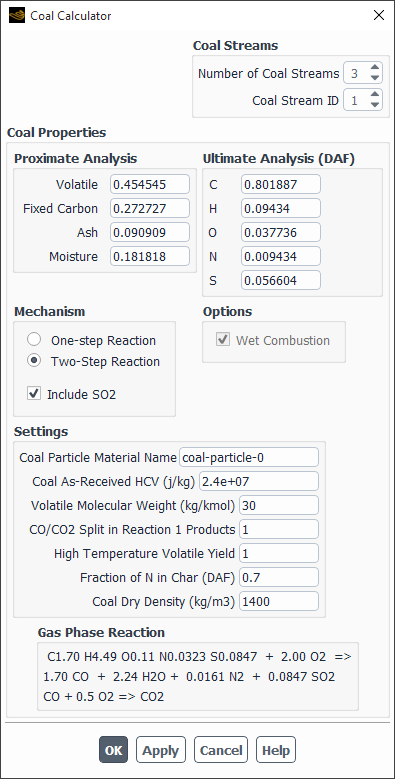
Controls
- Coal Streams
allows you to set up to three coal streams (Species Transport model only).
- Number of Coal Streams
specifies the total number of coal streams.
- ID
sets the ID of the coal stream for which you want to specify Coal Properties.
- Coal Properties
contains inputs for the current coal stream.
- Proximate Analysis
is the mass fraction of Volatile, Fixed Carbon, Ash, and Moisture in the coal.
- Volatile
is the fraction of the volatile component.
- Fixed Carbon
is calculated as one minus the sum of the actual Volatile, Ash, and Moisture fractions.
- Ash
is the fraction of ash.
- Moisture
is the moisture fraction in the coal.
- Ultimate Analysis (DAF)
is the mass fraction of atomic C, H, O, N and optionally S, in the Dry-Ash-Free (DAF) coal.
- Mechanism
allows you to set the mechanisms.
- Secondary Stream
when enabled, allows you to set the two mixture fraction model with the primary stream representing char as
 , and
an empirical secondary stream representing the volatiles. This is
available when using the non-premixed combustion model.
, and
an empirical secondary stream representing the volatiles. This is
available when using the non-premixed combustion model.- One-step Reaction
is defined in Equation 19–6.
- Two-step Reaction
involves oxidation of volatiles to CO in the first reaction and oxidation of CO to CO2 in the second reaction, as described in Equation 19–7.
- Include SO2
when enabled, allows you to specify the atomic mass fraction of sulphur, S, which appears under Ultimate Analysis.
- Options
- Wet Combustion
when enabled will enable the DPM Wet Combustion option by default in all injections created after the button is clicked in the Coal Calculator dialog box.
- Settings
is where you will specify the values used in the calculation.
- Coal Particle Material Name
is the name of the DPM combusting particle material. The default name is coal-particle.
- Coal As-Received HCV
is the higher caloric value of the coal.
- Volatile Molecular Weight
is the molecular weight of pure volatiles.
- CO/CO2 Split in Reaction 1 Products
can be used to specify the molar fraction of CO to CO2 in the first reaction of Equation 19–7. The default value of 1 implies that all carbon is reacted to CO, with no CO2 produced.
- High Temperature Volatile Yield
is where the enhanced devolatization at higher temperatures can cause the volatile yield to exceed the proximate analysis fraction.
- Fraction of N in Char (DAF)
is used in calculating the split of atomic nitrogen for the Fuel NOx model.
- Coal Dry Density
is used to calculate the Volume Fraction of liquid-water for the Wet Combustion option in the Injections dialog box.
- Gas Phase Reaction
lists the reaction based on your entries for the proximate and ultimate analyses.
The Integration Parameters dialog box (opened by clicking
Integration Parameters... in the Species Model dialog
box) allows you to set the parameters for the integration of the chemical source term
 in Equation 7–157 in the Theory Guide. See Using ISAT for details.
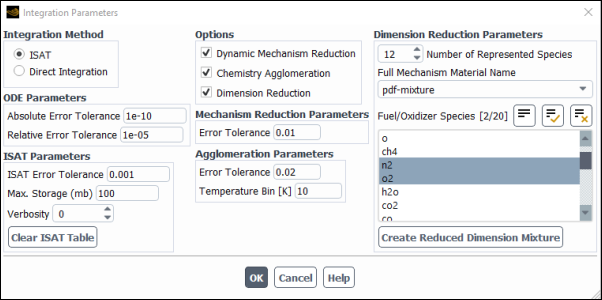
- Integration Method
contains options to choose the method for integration.
- ISAT
enables the ISAT option and expands the dialog box to include inputs for ISAT Parameters.
- Direct Integration
enables the direct integration method to integrate the chemical source term in the calculation.
- ODE Parameters
contains options to specify the error tolerances.
- Absolute Error Tolerance
specifies the absolute error tolerance.
- Relative Error Tolerance
specifies the relative error tolerance.
- ISAT Parameters
contains inputs required for ISAT integration method.
- ISAT Error Tolerance
controls the numerical error in ISAT liner interpolation. Decrease this value to get accurate minor species and pollutant predictions.
- Max. Storage
is the maximum RAM used by the ISAT table, and has a default value is 100 MB.
- Verbosity
specifies the level of detail at which you can monitor the ISAT performance.
- Clear ISAT Table
purges the ISAT table.
- Options
contains options to choose the method for chemistry acceleration.
- Dynamic Mechanism Reduction
accelerates chemistry by reducing the chemical kinetics mechanism on-the-fly to include only important species and reactions, with a corresponding decrease in accuracy. This method is available for single-phase flow simulations with Stiff Chemistry Solver only.
- Chemistry Agglomeration
when enabled, provides additional run-time improvement, with a corresponding decrease in accuracy. This method is available for Stiff Chemistry Solver (single-phase flow) and Relax to Chemical Equilibrium only.
- Dimension Reduction
is a chemistry acceleration method in addition to ISAT storage-retrieval and Cell Agglomeration, providing faster chemistry calculations with a corresponding loss of accuracy. This method is available for single-phase flow simulations with Stiff Chemistry Solver only.
- Dynamic Cell Clustering
enables a computationally efficient dynamic cell clustering method (DCC) that groups computational cells of high similarity into clusters using two DCC parameters:
Max. Temperature Dispersion (default =10 K)
Max. Equiv. Ratio Dispersion (default =0.05)
Max. Clusterization (default = 10)
Min. Clusterization (default = 0)
Reactants Threshold (mass fraction) (default = 1e-09)
This option is enabled by default and recommended. It is available only with the CHEMKIN-CFD Solver.
- Dynamic Adaptive Chemistry
accelerates chemistry by reducing the chemical kinetics mechanism on-the-fly to locally valid smaller mechanisms, with a corresponding decrease in accuracy. The level of accuracy is controlled by DAC Error Tolerance. You can select the initial target species to be tracked by the DAC algorithm in the Select DAC Target Species dialog box that opens when you click . See Using Dynamic Adaptive Chemistry with Ansys Fluent CHEMKIN-CFD Solver for more details.
This option is available only with the CHEMKIN-CFD Solver.
- Agglomeration Parameters
contains settings for the agglomeration chemistry method.
- Error Tolerance
determines the size of the clusters for species. By default, the value is 0.05.
- Temperature Bin
specifies the maximum bin size for temperature. The default value is 100 K.
- Dimension Reduction Parameters
contains settings to accelerate the chemistry.
- Number of Represented Species
must be greater than 10 and less than the number of species in the full mechanism. The Number of Represented Species must also be less than 50 minus the number of unrepresented elements (the number of chemical elements in the unrepresented species).
- Full Mechanism Material Name
is typically the name of the CHEMKIN mechanism that you imported.
- Fuel/Oxidizer Species
is where the boundary and initial fuel and oxidizer, as well as product species, are set as represented species.
- Create Reduced Dimension Mixture
creates a new mixture material called
reduced-dimension-mixture, which contains the represented species as well as proxy ’species’ for the unrepresented elements.
The Flamelet 3D Surfaces dialog box allows you to display 2D plots and 3D surfaces showing the variation of species fraction or temperature with the mean mixture fraction or scalar dissipation. See Postprocessing the Flamelet Data for details.
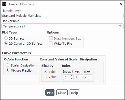
- Flamelet Type
indicates the type of flamelets whose surfaces will be displayed.
- Plot Variable
enables you to choose temperature or species fraction as the variable to be plotted.
- Plot Type
consists of options for plot type.
- 3D Surface
enables plotting on 3D surfaces.
- 2D curve on 3D surface
enables plotting of a 2D curve on a 3D surface.
- Options
consists of the following parameters:
- Draw Numbers Box
enables the display of a wireframe box with the numerical limits in each coordinate direction.
- Write To File
enables saving the plot data to a file.
- Curve Parameters
consists of controls related to plot display.
- X-Axis Function
consists of the function against which the plot variable will be displayed.
- Scalar Dissipation
enables display of plot variable against the scalar dissipation function.
- Mixture Fraction
enables display of plot variable against the mixture fraction.
- Constant Value of Scalar Dissipation
consists of the controls to specify the type of discretization (that is, how the flamelet data will be sliced) for the variable that is being held constant.
- Slice by
consists of the controls to specify discretization.
- Index
enables you to specify discretization index of the variable that is being held constant.
- Value
enables you to specify the numerical value of the variable that is being held constant.
- Index
consists of the controls that are displayed when you enable Index under Slice by.
- Index #
displays the index number.
- Min
displays the minimum of the range of integer values that you are allowed to choose from.
- Max
displays the maximum of the range of integer values that you are allowed to choose from.
- Value
consists of the controls that are displayed when you enable Value under Slice by.
- Value
enables you to enter the numerical value of the variable that is being held constant.
- Min
displays the minimum of the range of integer values that you are allowed to choose from.
- Max
displays the minimum of the range of integer values that you are allowed to choose from.
The Flamelet 2D Curves dialog box allows you to display or write 2D curves of the unsteady flamelets or strained flamelets. See Postprocessing the Flamelet Data or Modeling Strained Laminar Flame Speed, respectively, for details.
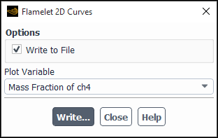
- Write to File
when enabled, write 2D curves to a file that you specify. When this option is selected, the Plot button will change to Write.... Clicking Write... opens the Select File dialog box (The Select File Dialog Box) where you can specify a name and save a file containing the plot data.
- Plot Variable
(non-premixed combustion flamelet model only) consists of a drop-down list of variables that you can plot or write.
- Flamelet Variable
(partially-premixed combustion FGM only) displays the Flame Speed flamelet variable that you can plot or write to file.
- Curve Parameters
(partially-premixed combustion FGM model only) consists of controls related to plot display.
- X-Axis Function
consists of the function against which the plot variable will be displayed.
- Strain Rate
enables display of plot variable against the strain rate function.
- Mixture Fraction
enables display of plot variable against the mixture fraction.
- Slice by
consists of the controls to specify discretization.
- Index
enables you to specify discretization index of the variable that is being held constant.
- Value
enables you to specify the numerical value of the variable that is being held constant.
- Index
consists of the controls that are displayed when you enable Index under Slice by.
- Index #
displays the index number.
- Min
displays the minimum of the range of integer values that you are allowed to choose from.
- Max
displays the maximum of the range of integer values that you are allowed to choose from.
- Plot
displays a plot of 2D curves of the flamelets in the active graphics window. When the Write to File option is selected, the Plot button changes to a Write....
The Unsteady Flamelet Parameters dialog box (opened by clicking Set Flamelet Parameters in the Flamelet tab of the Species Model dialog box) allows you to specify the initiation time of the unsteady flamelets. See Using the Diesel Unsteady Laminar Flamelet Model for details.
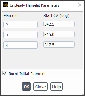
- Start CA (deg)
is the time at which each unsteady laminar flamelet will be generated during your simulation. The time is specified in terms of seconds or degrees of crank angle if the dynamic mesh is enabled.
- Burnt Initial Flamelet
if enabled, sets the initial flamelet condition to a chemical equilibrium burnt state. Otherwise, the initial flamelet condition is set to unburnt state (default).
The Flamelet Fluid Zones dialog box allows you to select the fluid zones for computing zone-averaged pressure and scalar dissipation. The dialog box is opened by clicking Set Flamelet Fluid Zones in the Flamelet tab of the Species Model dialog box. See Using the Diesel Unsteady Laminar Flamelet Model for details.
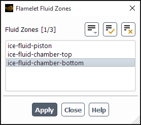
- Fluid Zones
is a selectable list of the fluid zones over which the average pressure and scalar dissipation are computed.
The Select Transported Scalars dialog box (opened by clicking FGM Scalar Transport in the Table tab of the Species Model dialog box) allows you to select the species for which transport equations will be solved. See Calculating the Look-Up Tables for more information about the items below.
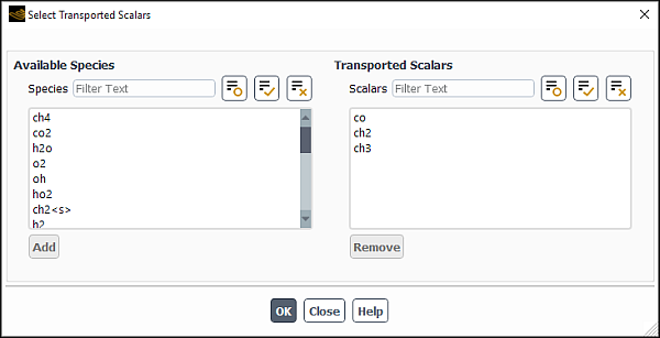
Controls
- Available Species
is a list of species available in the FGM flamelet table (either generated or imported). To add a species to the Transported Scalars list, select it in the Available Species multiple-selection list and click Add.
- Transported Scalars
is a list of selected species for which the transport equations will be solved, as described in Scalar Transport with FGM Closure in the Fluent Theory Guide. To remove a species from the Transported Scalars list back to the Available Species multiple-selection list, select it and click Remove.
The Distribution of Points dialog box (opened by clicking Edit... next to the chosen parameter either in the Flamelet tab or in the Table tab of the Species Model dialog box) allows you to edit the grid distribution for a chosen parameter (only for partially premixed combustion cases with FGM). See Editing the Flamelet Grid Distribution for more information about the items below. See also Premixed Flamelet Generated Manifolds, Diffusion Flamelet Generated Manifolds, and Calculating the Look-Up Tables for additional information.
Note that the default grid distributions for flamelet and table parameters are sufficient for most of the cases and should not be modified. However, in very specific cases, changing the grid distribution may improve accuracy.
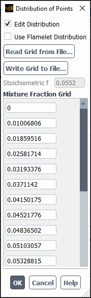
Controls
- Edit Distribution
enables you to edit the points of the grid distribution for the chosen parameter.
- Use Flamelet Distribution
allows you to use the points of the grid distribution of the FGM flamelet. This item is available only for the mixture fraction table parameter.
allows you to import a previously saved distribution point file into your case.
allows you to export the grid point data to an ASCII file in the XY plot file format.
- Stoichiometric f
displays the value of the stoichiometric mixture fraction. This is an information box; you cannot edit this value.
-
ParameterGrid displays the values of the points of the grid distribution. (The name of the chosen parameter will replace
ParameterinParameterGrid).
You can display 2D plots and 3D surfaces showing the variation of species mole fraction, density, or temperature with the mean mixture fraction, mixture fraction variance, or enthalpy. For the Flamelet Generated Manifold (FGM) model, additional variables are available for generating plots for PDF lookup tables. See Postprocessing the Look-Up Table Data for details about the items below.
The PDF Table dialog box can be accessed in one of two ways:
by clicking the button in the Table tab of the Species Model dialog box (as shown in Figure 20.23: The Species Model Dialog Box (Table) Tab Excluding Automated Grid Refinement)
by using the following path:
 Postprocessing → Model Specific
→ PDF Table...
Postprocessing → Model Specific
→ PDF Table...
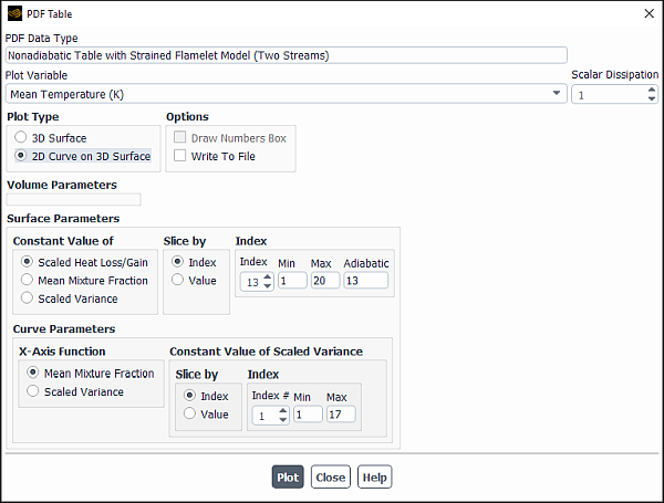
Controls
- PDF Data Type
describes the system that you are displaying.
- Plot Variable
is a drop-down list from which you can select temperature, density, or species mass fraction as the variable to be plotted. For the FMG model, you can also select mean rate of reaction progress.
-
Enthalpy Slice, Adiabatic =
slice number (FGM model only) specifies the value of the enthalpy slice level. By default, the enthalpy level is fixed at the adiabatic level displayed in the label as Adiabatic =
slice number. Enthalpy slice numbers below the adiabatic slice number are associated with heat loss, while enthalpy slice numbers above the adiabatic slice number are associated with enthalpy gain.- Scalar Dissipation
(multiple flamelets only) specifies the value of the Scalar Dissipation.
- Plot Type
gives you the choice of plotting a 3D surface or a slice of a 3D surface.
- 3D Surface
displays a 3D plot of the variation of species mole fraction, density, or temperature with the mean mixture fraction, mixture fraction variance, or enthalpy.
- 2D Curve on 3D Surface
consists of a 2D curve that is a slice of a 3D surface.
- Options
contains options specific to the display of 3D surfaces or 2D curves on 3D surfaces.
- Draw Numbers Box
enabling this option displays a wireframe box with the numerical limits in each coordinate direction. This option is available only when 3D Surface is selected.
- Write To File
specifies whether you want to write the plot data to a file. This option is available only when 2D Curve on 3D Surface is selected. The Plot button changes to a button when this option is enabled.
- Volume Parameters
(FGM model only) contains settings for selecting and fixing a discrete independent variable.
- Constant Value of
contains the discrete independent variables that can be held constant in the lookup table. The choices are Mean Reaction Progress, Scaled Reaction Progress Variance, Mean Mixture Fraction, and Scaled Variance.
- Slice by
allows you to select whether the 3D array of data points available in the look-up table will be sliced by Index or Value.
- Index/Value
contains index/values and their ranges.
- Index/Value
allows you to specify the discretization index or numerical value of the variable that is being held constant.
- Min/Max
are the range of integer values that you are allowed to choose from or display.
- Surface Parameters
contains settings where discrete independent variables are held constant and where curve parameters are defined.
- Constant Value of
contains the discrete independent variables that can be held constant in the lookup table. The choices are Scaled Heat Loss/Gain, Mean Mixture Fraction, and Scaled Variance. For a two-mixture-fraction case, the Scaled Heat Loss/Gain is the only available option. For the FGM model, this group box contains the discrete independent variables that have not been fixed in the Volume Parameters group box.
- Slice by
allows you to select whether the 3D array of data points available in the look-up table will be sliced by Index or Value.
- Index/Value
contains index/values and their ranges.
- Index/Value
allows you to specify the discretization index or numerical value of the variable that is being held constant.
- Min/Max
are the range of integer values that you are allowed to choose from or display.
- Adiabatic
is the enthalpy slice index corresponding to the adiabatic case for which the enthalpy (Scaled Heat Loss/Gain) is held constant.
- Curve Parameters
allows you to specify the X-Axis Function against which the plot variable will be displayed when 2D Curve on 3D Surface is selected.
- X-Axis Function
contains the remaining discrete independent parameters that have not been fixed yet.
-
Constant Value of
Independent Parameter allows you to specify the type of discretization for the variable that is being held constant using the controls in the Slice by and Index/Value group boxes. These items are similar to those described above.
- Display
displays the plot variable of the 3D surface.
plots the plot variable for the 2D curve on 3D surface.
opens The Select File Dialog Box where you will specify a name for the file containing plot data. This button appears when Write To File is enabled for the 2D Curve on 3D Surface plot type.
The Spark Ignition dialog box allows you to define multiple sparks (see Using the Spark Model for details).
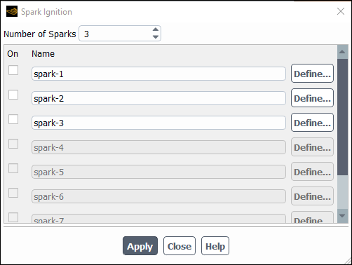
Controls
- Number of Sparks
is the quantity of sparks you would like to include in your simulation. You can define up to 16 sparks.
- On
if enabled, turns on those sparks that will be included in the simulation.
- Name
is the name of the spark. You can specify a name, or use the default name.
- Define...
opens the Set Spark Ignition Dialog Box.
The Set Spark Ignition dialog box allows you to set the parameters related to the spark ignition model (see Using the Spark Model for details).
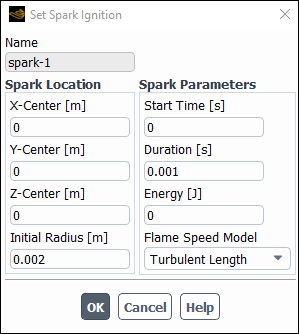
Controls
- Name
displays the name of the spark being defined.
- Spark Location
contains the parameters needed to define the location and size of the spark.
- X, Y, and Z-Center
specifies x, y, and z coordinates of the spark center.
- Initial Radius
specifies the initial spark radius.
- Spark Parameters
contains the parameters needed to define the spark.
- Start Time
is the time of spark ignition initialization in seconds. When the in-cylinder model is turned on, this control is replaced by the Start Crank Angle control.
- Start Crank Angle
is the time of spark ignition initialization in crank angle degrees. When the in-cylinder model is turned off, this control is replaced by the Start Time option.
- Duration
is the duration of the spark ignition in seconds.
- Energy
contains the total energy input by the spark. The default energy value is 0. A positive value for energy will cause the temperature of the spark kernel to rise above the combustion process temperature.
- Flame Speed Model
allows you to select the turbulent flame speed model for controlling the rate at which the flame front moves.
- Turbulent Curvature
includes the effect of flame curvature as specified in Turbulent Curvature in the Fluent Theory Guide.
- Turbulent Length
neglects the effects of flame curvature on the flame speed as described in Turbulent Length in the Fluent Theory Guide.
- Herweg-Maly
calculates the turbulent flame speed using Herweg-Maly model. See Herweg-Maly in the Fluent Theory Guide for details.
- Laminar
specifies the turbulent flame speed as the laminar flame speed. This option can be used to apply user-defined function (UDF) for the turbulent flame speed definition.
The Autoignition Model dialog box allows you to set the parameters related to the Knock Model or the Ignition Delay Model. See Modeling Engine Ignition for details.
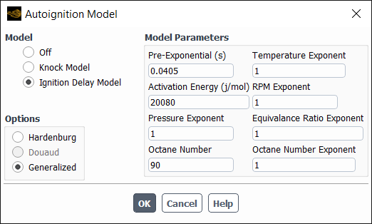
Controls
- Model
contains options to disable or enable models.
- Off
disables the model.
- Knock Model
enables the knock model. With the Premixed Combustion or Partially Premixed Combustion models selected, only the Knock Model can be turned on.
- Ignition Delay Model
enables the ignition delay model.
- Options
contains two correlation options that exist with each model.
- Douaud
option is used for knock in spark ignition engines. The modeling parameters that are specified for this option are the Pre Exponential, Pressure Exponent, Activation Temperature, Octane Number, and Octane Exponent (Equation 10–8 in the Theory Guide).
- Generalized
enables generalized correlation described by Equation 10–9 in the Theory Guide. It requires the same parameters as in the ignition delay model.
- Hardenburg
enables Hardenburg correlation, which is used for heavy-duty diesel engines. This option is enabled only for the ignition delay model.
- Model Parameters
contains parameters related to the selected model. See Using the Autoignition Models for the details about the parameters in this dialog box.
- Pre-Exponential
see Equation 10–9 and Equation 10–8 in the Theory Guide.
- Activation Temperature
see Equation 10–8 in the Theory Guide.
- Pressure Exponent
see Equation 10–9 and Equation 10–8 in the Theory Guide.
- Octane Number
see Equation 10–9 and Equation 10–8 in the Theory Guide.
- Octane Number Exponent
see Equation 10–9 and Equation 10–8 in the Theory Guide.
- Activation Energy
see Equation 10–9 and Equation 10–11 in the Theory Guide.
- Temperature Exponent
see Equation 10–9 in the Theory Guide.
- RPM Exponent
see Equation 10–9 in the Theory Guide.
- Equivalence Ratio Exponent
see Equation 10–9 in the Theory Guide.
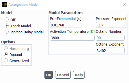
The Inert dialog box allows you to set the parameters related to the inert model. For details, see Setting Up the Inert Model.
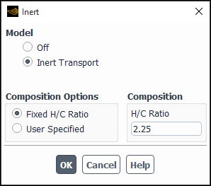
Controls
- Model
allows you to enable or disable the inert model.
- Off
disables the model.
- Inert Transport
enables the inert model.
- Composition Options
allows you to select a fixed H/C ratio or to specify the composition.
- Fixed H/C Ratio
allows you to specify a fixed ratio of hydrogen to carbon in the H/C Ratio field.
- User Specified
allows you to specify an arbitrary composition for the inert stream.
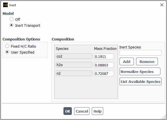
- Composition
allows you to set the H/C ratio or the mass fraction.
When Fixed H/C Ratio is selected under Composition Options, the following option(s) are available:
- H/C Ratio
specifies the fixed ratio of hydrogen to carbon when the Fixed H/C Ratio option is enabled.
When User Specified is selected under Composition Options, the following option(s) are available:
- Species
lists the inert species name.
- Mass Fraction
displays the mass fraction of the corresponding species.
- Inert Species
allows you to specify the name of the inert species.
- Add
adds the specified inert species to the species list.
- Remove
removes the specified inert species from the species list.
- Normalize Species
makes sure the species mass fractions add up to 1.
- List Available Species
lists all species in the thermodynamic database file (
thermo.db) in the console window,
The NOx Model dialog box allows you to set parameters related to the NOx postprocessor. See Using the NOx Model for details about the items below.
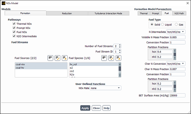
Controls
- Models
contains tabs for defining the models used to calculate the NOx production.
- Formation
contains the parameters to define the NOx model formation.
- Pathways
contains toggle buttons for enabling the NOx models to be used for the calculation of NO and HCN concentrations.
- Thermal NOx
enables calculation of thermal NOx.
- Prompt NOx
enables the calculation of prompt NOx.
- Fuel NOx
enables the calculation of fuel NOx. When using the non-premixed combustion model, the Fuel NOx option is only available if the DPM model is also enabled.
- N2O Intermediate
enables the formation of NOx through an N2O intermediate. This option will only appear if one of the previously listed NOx models is enabled.
- Fuel Streams
allows you to define multiple fuel streams for prompt NOx and fuel NOx formation.
- Number of Fuel Streams
sets the number of fuel streams. You are allowed up to three fuel streams.
- Fuel Stream ID
specifies the fuel stream you are defining in the PDF Stream drop-down list, the Fuel Species selection list, the Prompt tab, and the Fuel tab.
- PDF Stream
specifies the PDF stream species associated with a particular Fuel Stream ID, when calculating fuel NOx formation in conjunction with the non-premixed combustion model. You can select either the primary or secondary fuel streams, as defined in the PDF table.
- Fuel Species
is a list containing all of the defined species, which allows you to specify the species that is the fuel associated with a particular Fuel Stream ID. You cannot select more than 5 fuel species for each fuel stream, and the total number of fuel species selected for all the fuel streams combined cannot exceed 10. Note that when the non-premixed combustion model is enabled, your selection in the Fuel Species list only applies to prompt NOx calculations.
- Fuel Sources
is a list containing all of the fuel N sources. This list is available when Fuel NOx is enabled and your case contains injections with different DPM materials defined, such as combusting particles and droplets.
- User-Defined Functions
contains the NOx Rate drop-down list, which allows you to use a user-defined function (UDF) to contribute to the rate of NOx production. See the separate Fluent Customization Manual for details. Note that you may also use a UDF to specify custom values for the maximum limit (
 )
that is used for the integration of the temperature PDF (when temperature
is accounted for in the turbulence interaction modeling).
)
that is used for the integration of the temperature PDF (when temperature
is accounted for in the turbulence interaction modeling).
- Reduction
allows you to specify the reduction methods.
- Methods
contains the list of reduction methods.
- Reburn
enables the calculation of NOx reburning effects.
- SNCR
enables the calculation of NOx reduction by the SNCR method.
- Turbulence Interaction Mode
contains parameters related to the effect of turbulent fluctuations on the NOx formation. See NOx Formation in Turbulent Flows in the Theory Guide for details.
- PDF Mode
is a drop-down list containing options that take into account turbulent fluctuations when you compute the specified NOx formation. See Setting Turbulence Parameters for details.
- none
specifies the use of laminar NOx rate calculations, so that the effects of turbulence are ignored.
- temperature
includes fluctuations of temperature.
- temperature/species
includes fluctuations of the temperature and the mass fraction of the species selected in the Species drop-down list (which appears when you select this option).
- mixture fraction
includes fluctuations of the mixture fraction(s). This is available for non-premixed combustion calculations only.
- PDF Type
allows you to specify the shape of the PDF.
- beta
models the PDF using Equation 9–108 in the Theory Guide.
- gaussian
models the PDF using Equation 9–111 in the Theory Guide.
- PDF Points
controls the number of points at which the beta function in Equation 9–105 or Equation 9–106 in the Theory Guide will be integrated. The default value of 10, which indicates that the beta function will be integrated at 10 points on a histogram basis. The default value should yield an accurate solution with a reasonable computation time. Increasing this value may improve accuracy, but will also increase the computation time. This field is only available when temperature or temperature/species is selected from the PDF Mode drop-down list.
- Temperature Variance
allows you to specify the form of the transport equation that is solved to calculate the temperature variance.
- algebraic
is an approximate form of the transport equation (see Equation 9–114 in the Theory Guide).
- transported
solves Equation 9–113 in the Theory Guide.
- Tmax Option
provides various options for determining the maximum limit(s) for the integration of the PDF used to calculate the temperature.
- global-tmax
sets the limit as the maximum temperature in the flow field.
- local-tmax-factor
yields cell-based maximum temperature limits by multiplying the local cell mean temperature by the value entered in Tmax Factor.
- specified-tmax
sets the limit for each cell to be the value entered in Tmax.
- user-defined
allows you to hook a user-defined function that specifies custom values for the maximum limit (
 ), which is used for the integration of the temperature
PDF. This option is only available if you have already compiled a
user-defined function and selected it in the Formation tab.
), which is used for the integration of the temperature
PDF. This option is only available if you have already compiled a
user-defined function and selected it in the Formation tab.
- Species
is a drop-down list that appears when temperature/species is selected from the PDF Mode drop-down list. Here you will select the species whose mass fraction fluctuations will be factored into the NOx rate calculations.
- Formation Model Parameters
contains the tabs used to define the NOx pathways.
- Thermal
contains parameters for modeling thermal NOx. (The contents of this tab will appear only if Thermal NOx is enabled in the Formation tab.)
- [O ] Model
is a drop-down list in which you can select the method to be used for calculation of thermal NOx. To choose the equilibrium method, select equilibrium. To choose the partial equilibrium method, select partial-equilibrium. To choose the predicted O concentration method, select instantaneous. See Method 1: Equilibrium Approach, Method 2: Partial Equilibrium Approach, and Method 3: Predicted O Approach in the Theory Guide for details.
- [OH ] Model
is a drop-down list in which you can select the method to be used for calculation of thermal NOx. To exclude OH, select none. To choose the partial equilibrium method, select partial-equilibrium. To choose the predicted OH concentration method, select instantaneous. See Method 1: Exclusion of OH Approach, Method 2: Partial Equilibrium Approach, and Method 3: Predicted OH Approach in the Theory Guide for details.
- UDF Rate
provides options for the treatment of the NOx production specified by the user-defined function selected in the Formation tab.
- Replace Fluent Rate
replaces Ansys Fluent’s thermal NOx rate calculations with the custom NOx rate produced by your user-defined function.
- Add to Fluent Rate
adds the custom NOx rate produced by your user-defined function to Ansys Fluent’s thermal NOx rate calculations.
- Prompt
contains parameters for modeling prompt NOx. (The contents of this tab will appear only if Prompt NOx is enabled in the Formation tab.) The settings made in this tab will be associated with a particular fuel stream, specified in the Fuel Stream ID field in the Formation tab.
- Fuel Carbon Number
specifies the number of carbon atoms per fuel molecule.
- Equivalence Ratio
is the ratio of the actual fuel/air ratio to the stoichiometric fuel/air ratio.
- UDF Rate
provides options for the treatment of the NOx production specified by the user-defined function selected in the Formation tab.
- Replace Fluent Rate
replaces Ansys Fluent’s prompt NOx rate calculations with the custom NOx rate produced by your user-defined function.
- Add to Fluent Rate
adds the custom NOx rate produced by your user-defined function to Ansys Fluent’s prompt NOx rate calculations.
- Fuel
contains parameters for modeling fuel NOx. (The contents of this tab will appear only if Fuel NOx is enabled in the Formation tab.) The settings made in this tab will be associated with a particular fuel stream, specified in the Fuel Stream ID field in the Formation tab.
- Fuel Type
specifies the type of fuel NOx to be calculated.
- Solid
enables the calculation of solid fuel NOx.
- Liquid
enables the calculation of liquid fuel NOx.
- Gas
enables the calculation of gas fuel NOx.
- N Intermediate
allows you to specify any one of the hcn, nh3, or hcn/nh3/no as the intermediate species. See Fuel NOx Formation in the Theory Guide for details.
- Volatile N Mass Fraction
specifies the mass fraction of nitrogen in the volatiles. This parameter appears only for Solid fuel NOx calculations.
- Fuel N Mass Fraction
specifies the mass fraction of nitrogen in the fuel. This parameter appears only for Gas or Liquid fuel NOx calculations.
- Conversion Fraction
specifies the overall mass fraction of fuel N (for gas and liquid fuels), or volatile N or char N (for solid fuels), that will be converted to intermediate species and/or product NO.
- Partition Fractions
specifies the mass fraction of the converted fuel N (for gas and liquid fuels), or volatile N or char N (for solid fuels), that will become hcn and nh3. The fraction that will become NO will be calculated by the remainder. This option will appear only if you have selected hcn/nh3/no for the N Intermediate or Char N Conversion drop-down lists.
- Char N Conversion
is a drop-down list in which you can select no, hcn, nh3, or hcn/nh3/no as the species to which the char N is converted (when you are calculating solid fuel NOx). This parameter appears only for Solid fuel NOx calculations. See Setting Solid (Coal) Fuel NOx Parameters for details.
- Char N Mass Fraction
specifies the mass fraction of nitrogen in the char. This parameter appears only for Solid fuel NOx calculations.
- BET Surface Area
sets the BET internal pore surface area (see BET Surface Area in the Theory Guide for details) of the particles. This parameter appears only for Solid fuel NOx calculations.
- UDF Rate
provides options for the treatment of the NOx production specified by the user-defined function selected in the Formation tab.
- Replace Fluent Rate
replaces Ansys Fluent’s fuel NOx rate calculations with the custom NOx rate produced by your user-defined function.
- Add to Fluent Rate
adds the custom NOx rate produced by your user-defined function to Ansys Fluent’s fuel NOx rate calculations.
- N2O Path
contains the method to be used for formation of NO through an N2O intermediate. (The contents of this tab will appear only if N20 Intermediate is enabled in the Formation tab.)
- N2O Model
contains the drop-down list of available N2O models.
- quasi-steady
enables the quasi-steady-state method of calculation (The transport equation for the species N2O will not be solved).
- transported-simple
enables the transported simple method of calculation (The pollutant species N2O is added in the species list and it’s mass fraction will be calculated using the transport equations).
- UDF Rate
provides options for the treatment of the NOx production specified by the user-defined function selected in the Formation tab.
- Replace Ansys Fluent Rate
replaces the NOx rate calculated by Ansys Fluent using N2O intermediates with the custom NOx rate produced by your user-defined function.
- Add to Ansys Fluent Rate
adds the custom NOx rate produced by your user-defined function to the NOx rate calculated by Ansys Fluent using N2O intermediates.
- Reduction Method Parameters
contains tabs that allow you to define the methods of reduction. (These tabs are do not appear unless a reduction method has been enabled in the Reduction tab.)
- Reburn
allows you to define the NOx reduction when Reburn is enabled in the Reduction tab.
- Reburn Model
contains the drop-down list of reburn methods.
- instantaneous[CH ]
enables the instantaneous method in the Reburn Model. When you choose this method a warning to include CH, CH2, and CH3 will be displayed.
- partial-equilibrium
activates partial method in the Reburn Model.
- Reburn Fuel Species
contains reburn fuel species drop-down list.
- Equivalent Fuel Type
contains equivalent fuel type drop-down list.
- SNCR
allows you to define the NOx reduction when SNCR is enabled in the Reduction tab.
- Injection Method
contains the parameters for NOx reduction by SNCR method.
- gaseous
includes ammonia or urea as a gas-phase pollutant species from the injection locations.
- liquid
includes ammonia or urea as a liquid-phase pollutant species from the injection locations.
- Reagent Species
allows you to specify the reagent species as either ammonia (nh3) or urea (co<nh2>2)
- Reagent Fraction in Stream
allows you to specify the mass fraction of the reagent in the reagent stream. The remaining mass fraction is assumed to be water. If you enabled a secondary stream in your PDF calculation, by default the secondary stream will act as the reagent stream. Note that the Reagent Fraction in Stream field is only available when using the non-premixed combustion model with a liquid-phase reagent injection.
- Urea Decomposition
allows you to specify the decomposition model to use when the selected Reagent Species is co<nh2>2.
- rate-limiting
specifies that the source terms be calculated according to the rates given in Table 9.3: Two-Step Urea Breakdown Process.
- user-specified
allows you to specify the molar conversion fraction for ammonia, assuming that the rest of the urea is converted to HNCO.
- NH3 Conversion
is the mole fraction of
 in the mixture of
  and HNCO instantly
created from the reagent injection. The NH3 Conversion field only appears when user-specified is selected
for Urea Decomposition.
and HNCO instantly
created from the reagent injection. The NH3 Conversion field only appears when user-specified is selected
for Urea Decomposition.
The Soot Model dialog box allows you to set parameters related to the soot model. See Using the Soot Models for details about the items below.
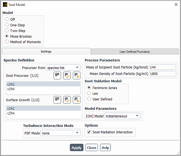
Controls
- Model
specifies which model should be used for computing soot formation.
- Off
disables the calculation of soot formation.
- One-Step
enables the one-step soot model described in The One-Step Soot Formation Model in the Theory Guide.
- Two-Step
enables the two-step soot model described in The Two-Step Soot Formation Model.
- Moss-Brookes
enables the Moss-Brookes soot model described in The Moss-Brookes Model in the Theory Guide.
- Moss-Brookes-Hall
enables the Moss-Brookes-Hall soot model described in The Moss-Brookes-Hall Model in the Theory Guide. This option is only available when C2H2, C6H6, C6H5, and H2 are present in the gas phase species list.
- Method of Moment
enables the Method of Moment soot model described in Setting Up the Method of Moments Soot Model.
- Species Definition
contains inputs for specifying the chemical species for your model.
- Fuel
is a drop-down list containing all of the defined species. Here you will select the species that is the fuel for the One-Step and Two-Step models, as well as the Moss-Brookes model when a precursor species is not identified in the defined species list.
- Oxidant
is a drop-down list containing all of the defined species. Here you will select the species that is the oxidizer for the One-Step and Two-Step models.
- Precursor from
allows you to select from a list of species, enter the correlation values of species, or enables you to hook a user-defined function, used to define the user defined precursor species. This selection is available when using the Moss-Brookes and Moss-Brookes-Hall models.
- User Defined Precursor
allows you to hook a user-defined function to specify the user defined soot precursor. This selection is available when using the Moss-Brookes and Moss-Brookes-Hall models.
- Soot Precursor
is a selection list containing all of the possible precursor species found via a query of the defined species list. By default, Ansys Fluent only considers
c2h2,c6h6, andc2h4as possible precursor species. For information about including other species in the possible precursor species search, contact your Ansys Fluent support engineer. From this list you will select the species that are the soot precursor species for the Moss-Brookes, Moss-Brookes-Hall, or Method of Moments models.- Surface Growth
is a selection list containing all of the possible surface growth species, as explained previously for the Soot Precursor selection list. Here you will select the species that are the surface growth species for the Moss-Brookes and Moss-Brookes-Hall models.
- Fuel Carbon Number
is the number of carbon atoms in the species selected in the Fuel drop-down list. This field appears only for the Moss-Brookes and Moss-Brookes-Hall model, when user-correlation is selected in the Precursor from drop-down list.
- Fuel Hydrogen Number
is the number of hydrogen atoms in the species selected in the Fuel drop-down list. This field appears only for the Moss-Brookes and Moss-Brookes-Hall model, when user-correlation is selected in the Precursor from drop-down list.
- Molecular Weight of Precursor
is the molecular weight of the precursor species. This field appears only for the Moss-Brookes and Moss-Brookes-Hall model, when user-correlation is selected in the Precursor from drop-down list. The default value is the weight of acetylene.
- Precursor Correlation
is a drop-down list you can use to define a laminar diffusion profile that relates mixture fraction to precursor mass fraction. This field appears only for the Moss-Brookes and Moss-Brookes-Hall model, when user-correlation is selected in the Precursor from drop-down list.
- piecewise-polynomial
specifies that the precursor mass fraction is a piecewise-polynomial function of mixture fraction. The default values used by Ansys Fluent correspond to a methane diffusion flame simulation, in which both the air and fuel initial temperatures are set to 290 K, and acetylene is assumed as the soot precursor. These values can be revised via the Edit... button.
- constant
specifies that the precursor mass fraction is a constant function of mixture fraction, the value of which is specified in the field below the Precursor Correlation drop-down list.
- Edit...
opens the Piecewise-Polynomial Profile Dialog Box when piecewise-polynomial is selected from the Precursor Correlation drop-down list, thus allowing you to revise the default values.
- Sticking Coefficients...
(only for the method of moments soot model) opens Sticking Coefficients Dialog Box where you can provide the correction factors to be used for calculating the nucleation rates. This button is available only when User Precursor is the selected soot nucleation model.
- Turbulence Interaction Mode
contains inputs that specify how turbulent fluctuations are accounted for in the soot formation calculations for the Moss-Brookes and Moss-Brookes-Hall models. For further details on these inputs, see Setting Up the Moss-Brookes Model and the Hall Extension.
- PDF Mode
is a drop-down list that contains the options for addressing turbulent fluctuations in the soot rate calculations. Note that mixture fraction is the most accurate option, and should be used if it is available.
- none
specifies the use of laminar soot rate calculations, so that the effects of turbulence are ignored.
- temperature
specifies that the soot rate calculations include the effect of temperature fluctuations.
- temperature/species
specifies that the soot rate calculations include the effect of fluctuations of temperature, as well as fluctuations of the mass fraction of the species selected in the Species drop-down list (which appears when you select this option).
- mixture fraction
is the most accurate option, specifying that the soot rate calculations include the effect of fluctuations of mixture fraction(s). Note that this option is not available if you are using the eddy-dissipation model.
- PDF Type
allows you to specify the shape of the PDF.
- beta
models the PDF using Equation 9–108 in the Theory Guide.
- gaussian
models the PDF using Equation 9–111 in the Theory Guide.
- PDF Points
controls the number of points at which the beta function will be integrated on a histogram basis. Increasing this number may improve accuracy, but will also increase compute time. This field is only available when temperature or temperature/species is selected from the PDF Mode drop-down list.
- Temperature Variance
allows you to specify the form of transport equation that is solved to calculate the temperature variance.
- algebraic
is an approximate form of the transport equation (see Equation 9–114 in the Theory Guide).
- transported
solves Equation 9–113 in the Theory Guide.
- Tmax Option
provides various options for determining the maximum limit(s) for the integration of the PDF used to calculate the temperature.
- global-tmax
sets the limit as the maximum temperature in the flow field.
- local-tmax-factor
yields cell-based maximum temperature limits by multiplying the local cell mean temperature by the value entered in Tmax Factor.
- specified-tmax
sets the limit for each cell to be the value entered in Tmax.
- user-defined
allows you to hook a user-defined function that specifies custom values for the maximum limit (
 ), which is used for the integration of the temperature
PDF. This option is only available if you have already compiled a
user-defined function.
), which is used for the integration of the temperature
PDF. This option is only available if you have already compiled a
user-defined function.
- Species
is a drop-down list which appears when temperature/species is selected from the PDF Mode drop-down list. Here you will select the species whose mass fraction fluctuations will be factored into the soot rate calculations.
- Process Parameters
contains parameters that control the combustion process modeling.
- Mean Diameter of Soot Particle
is the assumed average diameter of the soot particles in the combustion system. For the Two-Step model, it is used to compute the soot particle mass
 in Equation 9–123 in
the Theory Guide.
in Equation 9–123 in
the Theory Guide.- Mean Density of Soot Particle
is the assumed average density of the soot particles in the combustion system. For the Two-Step model, it is used to compute the soot particle mass
 in Equation 9–123 in the
Theory Guide. For the
Moss-Brookes and Moss-Brookes-Hall models, it is
in Equation 9–123 in the
Theory Guide. For the
Moss-Brookes and Moss-Brookes-Hall models, it is
 in Equation 9–130 and
 in Equation 9–133 in the
Theory Guide. The default value
supplied by Ansys Fluent is 1800 kg/m3 (as was used in the work
of Brookes and Moss [28]).
in Equation 9–133 in the
Theory Guide. The default value
supplied by Ansys Fluent is 1800 kg/m3 (as was used in the work
of Brookes and Moss [28]).- Normalization Parameter for Moments
(only for the method of moments soot model) is used to solve the normalized soot moment transport equations to minimize the numerical errors. The default value of this input is sufficient and you may not need to change this.
- Stoichiometry for Soot Combustion
is the mass stoichiometry
 in Equation 9–120 in the
Theory Guide, which computes the soot
combustion rate in the One-Step and Two-Step
models. The default value supplied by Ansys Fluent (2.6667) assumes that the soot is pure
carbon and that the oxidizer is O2.
in Equation 9–120 in the
Theory Guide, which computes the soot
combustion rate in the One-Step and Two-Step
models. The default value supplied by Ansys Fluent (2.6667) assumes that the soot is pure
carbon and that the oxidizer is O2.- Stoichiometry for Fuel Combustion
is the mass stoichiometry
 in Equation 9–120 in the
Theory Guide, which computes the soot
combustion rate in the One-Step and Two-Step
models. The default value supplied by Ansys Fluent (3.6363) is for combustion of propane
(C3H8) by oxygen
(O2).
in Equation 9–120 in the
Theory Guide, which computes the soot
combustion rate in the One-Step and Two-Step
models. The default value supplied by Ansys Fluent (3.6363) is for combustion of propane
(C3H8) by oxygen
(O2).- Mass of Incipient Soot Particle
is
 in Equation 9–131 and Equation 9–133, which is used in the Moss-Brookes and Moss-Brookes-Hall model computations. The default value supplied by Ansys Fluent (144
kg/mol) is the mass of 12 carbon atoms. Note that for the original
implementation of the Hall extension, the model assumed this mass
to be 100 carbon atoms.
in Equation 9–131 and Equation 9–133, which is used in the Moss-Brookes and Moss-Brookes-Hall model computations. The default value supplied by Ansys Fluent (144
kg/mol) is the mass of 12 carbon atoms. Note that for the original
implementation of the Hall extension, the model assumed this mass
to be 100 carbon atoms.
- Soot Oxidation Model
contains model options that determine the form of the soot oxidation term in the calculations of the Moss-Brookes and Moss-Brookes-Hall models.
- Fenimore-Jones
takes into account the soot oxidation due to the hydroxyl radical.
- Lee
takes into account the soot oxidation due to the hydroxyl radical and molecular oxygen.
- User Defined
enables you to select a user-defined function for soot oxidation rate. This selection is available when using the Moss-Brookes and Moss-Brookes-Hall models.
- Number of Moments
(only for the method of moments soot model) specifies the number of moments to be used in the Method of Moments soot model. Ansys Fluent will solve an equal number of moment transport equations. The default value of three moments works reasonably well for wide range of problems. You can specify up to six moments.
- Soot Nucleation Model
(only for the method of moments soot model) contains model options related to soot nucleation modeling.
- Use Precursor
enables you to define the precursor species. The nucleation rates are calculated considering coagulation between precursor species using kinetic theory.
- Specify Mechanism
enables you to specify nucleation in terms of reactions.
- User Defined Oxidation Rate
allows you to hook the user-defined function to specify the soot oxidation rate. This selection is available when using the Moss-Brookes and Moss-Brookes-Hall models.
- Model Parameters
contains parameters that control the soot formation model.
- Soot Formation Constant
is the parameter
 in Equation 9–117 in the Theory Guide. This item
appears only for the One-Step soot model.
in Equation 9–117 in the Theory Guide. This item
appears only for the One-Step soot model.- Equivalence Ratio Exponent
is the exponent
 in Equation 9–117 in the Theory Guide. This item
appears only for the One-Step soot model.
in Equation 9–117 in the Theory Guide. This item
appears only for the One-Step soot model.- Equivalence Ratio Minimum
and Equivalence Ratio Maximum are the minimum and maximum values of the fuel equivalence ratio
 in Equation 9–117
in the Theory Guide. Equation 9–117 will be solved only if Equivalence Ratio Minimum <
in Equation 9–117
in the Theory Guide. Equation 9–117 will be solved only if Equivalence Ratio Minimum <  < Equivalence Ratio Maximum; if
  is outside of this range, there is no soot
formation. This item appears only for the One-Step soot model.
is outside of this range, there is no soot
formation. This item appears only for the One-Step soot model.- Activation Temperature of Soot Formation Rate
is the term
 in Equation 9–117 in the Theory Guide. This item
appears only for the One-Step soot model.
in Equation 9–117 in the Theory Guide. This item
appears only for the One-Step soot model.- Magnussen Constant for Soot Combustion
is the constant
 used in the rate expressions governing the soot
combustion rate (Equation 9–119 and Equation 9–120) in the Theory
Guide. This item appears only for the One-Step and the Two-Step soot models. For the Two-Step model, this input will be called Magnussen
Constant for Soot and Nuclei Combustion.
used in the rate expressions governing the soot
combustion rate (Equation 9–119 and Equation 9–120) in the Theory
Guide. This item appears only for the One-Step and the Two-Step soot models. For the Two-Step model, this input will be called Magnussen
Constant for Soot and Nuclei Combustion.- Limiting Nuclei Formation Rate
is the limiting value of the kinetic nuclei formation rate
 in Equation 9–126 in the Theory Guide. Below
this limiting value, the branching and termination term, (
in Equation 9–126 in the Theory Guide. Below
this limiting value, the branching and termination term, ( ) in Equation 9–125 in the Theory Guide, is not
included. This item appears only for the Two-Step soot model.
) in Equation 9–125 in the Theory Guide, is not
included. This item appears only for the Two-Step soot model.- Nuclei Branching-Termination Coefficient
is the term
 in Equation 9–125 in the Theory Guide. This item
appears only for the Two-Step soot model.
in Equation 9–125 in the Theory Guide. This item
appears only for the Two-Step soot model.- Nuclei Coefficient of Linear Termination on Soot
is the term
 in Equation 9–125 in the Theory Guide. This item
appears only for the Two-Step soot model.
in Equation 9–125 in the Theory Guide. This item
appears only for the Two-Step soot model.- Pre-Exponential Constant of Nuclei Formation
is the pre-exponential term
 in the kinetic nuclei formation term, Equation 9–126 in the Theory Guide. This item
appears only for the Two-Step soot model.
in the kinetic nuclei formation term, Equation 9–126 in the Theory Guide. This item
appears only for the Two-Step soot model.- Activation Temperature of Nuclei Formation Rate
is the term
 in the kinetic nuclei formation term, Equation 9–126 in the Theory Guide. This item
appears only for the Two-Step soot model.
in the kinetic nuclei formation term, Equation 9–126 in the Theory Guide. This item
appears only for the Two-Step soot model.- Alpha for Soot Formation Rate
is
 , the constant in the soot formation rate
equation, Equation 9–123 Two-Step soot model.
, the constant in the soot formation rate
equation, Equation 9–123 Two-Step soot model.- Beta for Soot Formation Rate
is
 , the constant in the soot formation rate
equation, Equation 9–123 in the Theory
Guide. This item appears only for the Two-Step soot model.
, the constant in the soot formation rate
equation, Equation 9–123 in the Theory
Guide. This item appears only for the Two-Step soot model.- Magnussen Constant for Soot and Nuclei Combustion
is the constant
 used in the rate expressions
governing the soot combustion rate (Equation 9–119 and Equation 9–120 in the Theory Guide). This item appears only for
the One-Step and the Two-Step soot models.
used in the rate expressions
governing the soot combustion rate (Equation 9–119 and Equation 9–120 in the Theory Guide). This item appears only for
the One-Step and the Two-Step soot models.- [OH] Model
is a drop-down list that allows you to specify the method by which the OH radical concentration is calculated, that is, instantaneous or partial-equilibrium. This list appears only for the Moss-Brookes, Moss-Brookes-Hall, and Method of Moments soot models.
- [O] Model
is a drop-down list that specifies the method by which the O radical concentration is calculated, that is, equilibrium, partial-equilibrium, or instantaneous. This list appears only for the Moss-Brookes and the Moss-Brookes-Hall soot models, when you have selected partial-equilibrium for the [OH] Model.
Important: To use the concentration of OH or O predicted by the combustion model, select instantaneous for [OH] Model or [O] Model.
- User Defined Functions
contains the User Defined Soot MOM Rates drop-down list, which allows you to use a user-defined function (UDF) to specify soot nucleation, surface growth, and oxidation rates for soot moment equations. This item is available only for the Method of Moments soot model. See Hooking
DEFINE_SOOT_MOM_RATESUDFs in the Fluent Customization Manual for details.- Options
contains an option for modeling the effect of soot on a variable radiation absorption coefficient. This group box will appear only when one of the radiation models in the Radiation Model Dialog Box is active.
- Soot-Radiation Interaction
enables the soot-radiation interaction model described in The Effect of Soot on the Absorption Coefficient in the Theory Guide.
- Soot Surface Growth Options
(only for the method of moments soot model) contains a parameter for modeling the soot surface growth.
- Site Density
is the number of sites/cm2 available on the soot surface for surface growth and oxidation reactions with the method of moment soot model.
- Enable Aggregation Model
(only for the method of moments soot model) enables the modeling of soot aggregates.
- Critical diameter
is the value of the soot particle diameter above which the coagulation regime is switched from coalescent to aggregate.
- Fractal dimension
is the parameter that describes the aggregate nature. For soot particles, a value between 1.7 and 2.0 is found to be reasonably good.
The Sticking Coefficients dialog box allows you to set sticking coefficients for the soot model with method of moments. It is opened from the Soot Model Dialog Box. See Setting Up the Method of Moments Soot Model for details about using this dialog box.
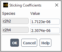
Controls
- Species
shows the name of the species for which you specify the Value.
The Mechanism dialog box allows you to set parameters related to nucleation reactions for the soot model with method of moments. It is opened from the Soot Model Dialog Box. See Setting Up the Method of Moments Soot Model for details about using this dialog box.
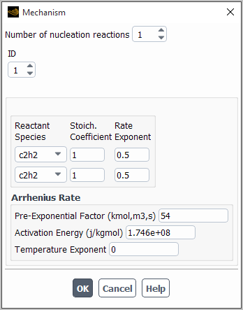
Controls
- Number of nucleation reactions
allows you to specify nucleation process as with a single or multi-step reaction mechanism. For each reaction, you must specify all appropriate reaction parameters.
- ID
displays the ID of the current nucleation reaction setup.
- Reactant Species
is a drop-down list that enables you to select the species for the current nucleation reaction.
- Stoich. Coefficient
specifies the stoichiometric coefficient of the reactant species in the nucleation reaction.
- Rate Exponent
specifies the rate constant for the reactant species in the current nucleation reaction.
- Arrhenius Rate
contains the inputs for the Arrhenius rate parameters related to the current nucleation reaction.
- Pre-exponential Factor
is the constant
 in Equation 7–23 in the
Theory Guide. The units of
in Equation 7–23 in the
Theory Guide. The units of
 must be specified such that the units of the molar reaction rate,
 (Equation 7–19 in the
Theory Guide, are moles/volume-time
(for example, kmol/m3-s) and the units of the volumetric
reaction rate,
(Equation 7–19 in the
Theory Guide, are moles/volume-time
(for example, kmol/m3-s) and the units of the volumetric
reaction rate,  in Equation 7–19 in the
Theory Guide, are mass/volume-time
(for example, kg/m3-s).
in Equation 7–19 in the
Theory Guide, are mass/volume-time
(for example, kg/m3-s).Important: It is important to note that if you have selected the British units system, the Arrhenius factor should still be specified in SI units. This is because Ansys Fluent applies no conversion factor to the value you enter for
 (the conversion factor is 1.0)
when you work in British units, as the correct conversion factor depends
on your values for
(the conversion factor is 1.0)
when you work in British units, as the correct conversion factor depends
on your values for  ,
,  , and so on.
- Activation Energy
is the constant
 in the forward rate constant
expression, Equation 7–23 in the Theory
Guide).
in the forward rate constant
expression, Equation 7–23 in the Theory
Guide).- Temperature Exponent
is the value for the constant
 in Equation 7–23 in the Theory Guide.
The Reactor Network dialog box allows you to set parameters related to the reactor network model and calculate the reactor network for species transport/combustion. See Reactor Network Model for details about using this dialog box.
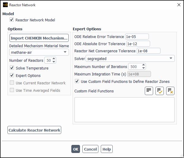
Controls
- Model
contains the option for enabling (or disabling) the reactor network model.
- Reactor Network Model
enables/disables the modeling of the reactor network.
- Options
contains the options for reactor network model. This portion of the dialog box appears only if Reactor Network Model is selected.
- Import CHEMKIN Mechanism
allows you to import a detailed chemical mechanism in CHEMKIN format.
- Detailed Mechanism Material Name
is a drop-down list of available mixture materials from which you can select a mixture material for your reactor network simulation.
- Number of Reactors
sets the number of reactors in which cells are grouped based on specified criteria.
- Solve Temperature
specifies whether or not the reactor network algorithm solves the temperature. By default, this option is selected.
- Expert Option
when selected, displays the advanced options related to the solver settings.
- Use Current Reactor Network
allows you to perform additional reactor network simulations with the existing network of connected reactors. This option can be enabled once the Fluent solver agglomerates cells and obtains the reactor-network solution.
- Use Time Averaged Fields
enables you to select the time-averaged composition fields to be used for clustering reactors and the time-averaged velocity fields for calculating reactor mass flux matrix. This option is available only for unsteady simulations with enabled Data Sampling For Unsteady Statistics option.
- Expert Options
contains advanced options for ODE solver and for reactor cell clustering control. This portion of the dialog box appears only if Expert Options is selected.
- ODE Relative Error Tolerance
specifies relative error control for ODE integrator.
- ODE Absolute Error Tolerance
specifies absolute error control for ODE integrator.
- Reactor Network Convergence Tolerance
allows you to specify tolerance to control the accuracy of the reactor network calculations.
- Solver
allows you to select the solver for your simulation. The default segregated solver typically converges faster than the coupled solver. However, if residuals stall above an acceptable tolerance, the coupled solver should be used.
- Maximum Number of Iterations
(segregated solver only) sets the maximum number of solver iterations.
- Maximum Integration Time
(coupled solver only) sets the maximum elapsed run time for ODE solver. Ansys Fluent terminates the run at this time if the residuals fail to converge.
- Use Custom Field Functions to Define Reactor Zones
enables the use of custom field functions (Custom Field Functions) for reactor network cell clustering.
- Custom Field Functions
contains the list of available user-defined field functions from which you can select the functions for reactor network cell clustering. This selection list will not appear if the Use Custom Field Functions to Define Reactor Zones option is not selected.
- Calculate Reactor Network
calculates a chemically reactive flow using reactor network model.
The Decoupled Detailed Chemistry dialog box allows you to postprocess slowly-forming, trace pollutant species on a steady-state flow field using detailed chemical kinetic mechanisms.
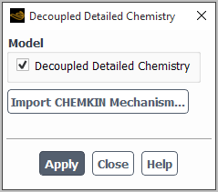
Controls
- Model
includes the option to enable Decoupled Detailed Chemistry.
- Import CHEMKIN Mechanism...
opens the Import CHEMKIN Format Mechanism Dialog Box.
- Integration Parameters...
opens the Integration Parameters Dialog Box.
- Original Species
are the species that are in the original case setup.
- Pollutant Species
are typically slowly forming (far from chemical equilibrium), and occur at miniscule mass fractions.
The Reacting Channel Model dialog box allows you to solve reacting flow in shell and tube heat exchangers with long and thin channels.
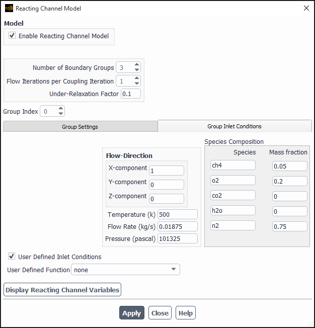
Controls
- Model
includes the option to Enable Reacting Channel Model.
- Number of Boundary Groups
allows you to group together channels with common flow direction, mixture materials, inlet compositions, temperature, pressure, and mass flow rate in cases where you have multiple channels.
- Flow Iterations per Coupling Iteration
is the number of outer flow iterations for each channel flow iteration.
- Under-Relaxation Factor
is used to update the heat flux from the reacting channel. See Equation 7–145 in the Theory Guide.
- Group Index
is used to identify the boundary group.
- Group Settings
contains Group Settings that you will set.
- Channel Walls in Group
are wall boundary zones that correspond to the reacting channels in the group.
- Material
is the group material.
- Import CHEMKIN Mechanism...
opens the Import CHEMKIN Format Mechanism Dialog Box.
- Model Options
allows you to enable Surface Reactions and Porous Medium models and set related parameters.
- Group Inlet Conditions
is where you specify the Temperature, the Flow Rate, the Pressure, and other inlet conditions of the reacting channel group.
- Flow Direction
is the X-, Y-, and Z-component of the flow at the inlets of the channels in the current group.
- Species Composition
is where you will specify the inlet mass fractions of the group.
- User Defined Inlet Conditions
enables you to hook a user-defined function to specify the reacting channel inlet conditions. When this option is selected, the User Defined Function drop-down list becomes visible.
- Display Reacting Channel Variables
opens the Reacting Channel 2D Curves Dialog Box for postprocessing reacting channel variables.
The Reacting Channel 2D Curves dialog box allows you to display or write 2D curves of the reacting channel.
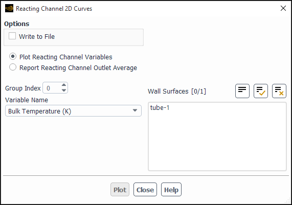
Controls
- Options
gives you the option to Plot, Report, or Write to File channel variables.
- Group Index
is used to identify the reacting channel boundary group.
- Plot Reacting Channel Variables
enables the plotting of reacting channel variables.
- Report Reacting Channel Outlet Average
enables the reporting of reacting channel outlet average.
- Variable Name
specifies the channel variable for plotting.
- Variable Names
contains a selectable list of channel variables for reporting.
- Wall Surfaces
contains a selectable list of wall surfaces on which you can plot, report or write the selected channel variables.
generates an X-Y plot. The button is available when Plot Reacting Channel Variables is selected. When the Write to File option is enabled, the Plot button changes to the Write... button.
generates the report of the channel variables. The button is available when Report Reacting Channel Outlet Average is selected. When the Write to File option is enabled, the Report button changes to the Write... button.
The Discrete Phase Model dialog box allows you to set parameters related to the calculation of a discrete phase of particles. See Modeling Discrete Phase for details.
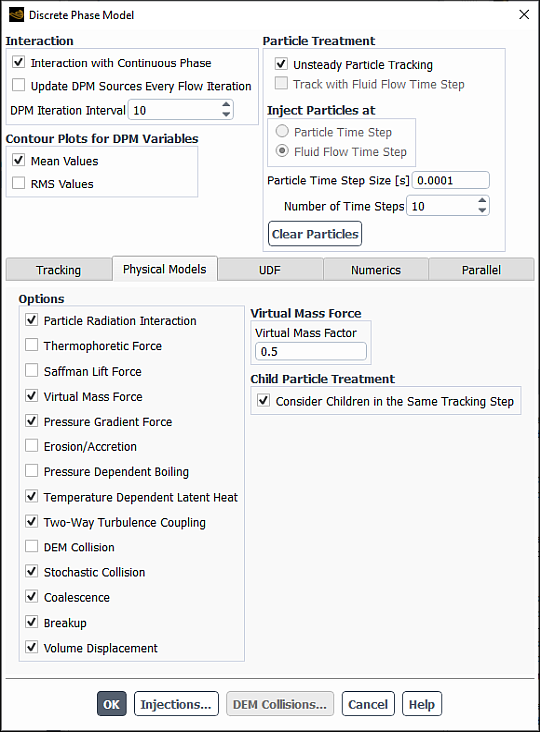
Controls
- Interaction
contains parameters used for performing coupled calculations of the continuous and discrete phase flow. See Procedures for a Coupled Two-Phase Flow for details.
- Interaction with Continuous Phase
enables a coupled calculation of the discrete phase and the continuous phase.
- Update DPM Sources Every Flow Iteration
when enabled, particle source terms will be updated according to Equation 24–14 at every flow iteration. For unsteady simulations, it is the default and is recommended.
- DPM Iteration Interval
allows you to control the frequency at which the particles are tracked and the DPM sources are updated.
- Contour Plots for DPM Variables
contains options for enabling cell-averaged discrete phase variables for postprocessing.
- Mean Values
enables additional cell-averaged discrete phase variables for postprocessing.
- RMS Values
enables additional RMS values for several discrete phase variables for postprocessing.
- Particle Treatment
contains options for choosing to treat the particles in an unsteady or a steady fashion.
- Unsteady Particle Tracking
enables unsteady tracking of particles.
- Track with Fluid Flow Time Step
enables the use of fluid flow time steps to inject the particles.
- Inject Particles at
contains parameters to decide when to inject the particles for a new time step.
- Particle Time Step
enables injection of particles for every particle time step.
- Fluid Flow Time Step
enables injection of particles for every fluid flow time step.
In any case, the particles will always be tracked in such a way that they coincide with the flow time of the continuous flow solver, as long as the Max. Number of Steps (in the Tracking tab) used to compute a single trajectory is sufficient.
- Particle Time Step Size
specifies particle time step size for the calculation.
- Number of Time Steps
allows you to specify the number of time steps for the calculation.
- Clear Particles
clears the particles that are currently in the domain.
- Tracking
contains settings to control the time integration of the particle trajectory equations and particle tracking.
- Tracking Parameters
contains parameters that control the tracking of particle trajectories. For steady-state particle tracking, one simple rule of thumb to follow when setting the two parameters below is that if you want the particles to advance through a domain of length
 , the Length Scale times the number of Max. Number of Steps should
be approximately equal to
, the Length Scale times the number of Max. Number of Steps should
be approximately equal to  . See Integration of Particle Equation of Motion in the Theory Guide for
details about the items below.
. See Integration of Particle Equation of Motion in the Theory Guide for
details about the items below.- Max. Number of Steps
is the maximum number of time steps used to compute a single particle trajectory via integration of Equation 12–1 in the Theory Guide and Equation 12–35. The default value is 50,000 for steady-state particle tracking and 500 for unsteady particle tracking.
- Specify Length Scale
when enabled allows you to specify the length scale.
- Length Scale
controls the integration time step size used to integrate the equations of motion for the particle. It appears only when the Specify Length Scale option is enabled.
- Step Length Factor
specifies the value of
 in Equation 24–3.
- Tracking Option
- High-Res Tracking
is a particle tracking algorithm that tracks particles through cells decomposed into tetrahedra (subtets). See Tracking Settings for the Discrete Phase Model for more information about this method.
- Physical Models
contains optional discrete phase models and their relevant parameters.
- Options
contains additional models that can be included in the calculation. See Physical Models for the Discrete Phase Model for more information.
- Particle Radiation Interaction
includes the effect of radiation heat transfer to the particles (Equation 5–73 in the Theory Guide). You will also need to define additional properties for the particle materials (emissivity and scattering factor), as described in Description of the Properties.
This item appears only if the P-1 or discrete ordinates model is selected in the Radiation Model Dialog Box.
- Thermophoretic Force
enables the inclusion of a thermophoretic force on the particles as an additional force term. See Thermophoretic Force in the Theory Guide for details.
- Saffman Lift Force
enables the inclusion of Saffman’s lift force (lift due to shear) as an additional force term. See Saffman’s Lift Force in the Theory Guide for details.
- Virtual Mass Force
enables the inclusion of virtual mass forces in the particle force balance. See Including the Virtual Mass Force and Pressure Gradient Effects on Particles for details.
- Pressure Gradient Force
enables the inclusion of pressure gradient effects in the particle force balance. See Including the Virtual Mass Force and Pressure Gradient Effects on Particles for details.
- Erosion/Accretion
enables the monitoring of erosion/accretion rates at wall boundaries. See Monitoring Erosion/Accretion of Particles at Walls for details.
- Pressure Dependent Boiling
allows you to switch from droplet vaporization (Law 2) to boiling (Law 3), as described in Considering Pressure Dependence in Boiling.
- Temperature Dependent Latent Heat
allows you to include the droplet temperature effects on the latent heat, as described in Equation 12–92 in the Theory Guide.
- Two-Way Turbulence Coupling
enables the effect of change in turbulent quantities due to particle damping and turbulence eddies. See Including the Effect of Particles on Turbulent Quantities for more information.
- DEM Collision
allows you to model DEM collision as described in Modeling Collision Using the DEM Model.
- Stochastic Collision
enables the effect of droplet collisions, as described in Collision and Droplet Coalescence Model Theory in the Theory Guide.
- Coalescence
enables the effect of droplet coalescence, as described in Collision and Droplet Coalescence Model Theory in the Theory Guide. This option is available when the Stochastic Collision option is enabled.
- Breakup
enables breakup for all suitable injections. You can select the breakup model and parameters, or disable breakup, for each injection in the Set Injection Properties Dialog Box.
- Volume Displacement
enables the volume displacement of particles, as described in Including the Volume Displacement of Particles.
- Child Particle Treatment
contains an option to Consider Children in the Same Tracking Step. This control appears only when either Breakup is enabled under Options or wall-film is selected for Discrete Phase BC Type in the DPM tab of the Wall dialog box.
- DEM Collision Model
contains model settings that allow you to continue your setup of the model.
- Adaptive Collision Mesh Width
is enabled by default. This adjusts the width of the collision mesh to the largest parcel diameter multiplied by the Edge Scale Factor
- Edge Scale Factor
is the factor by which the width of the collision mesh is adjusted to the largest parcel diameter.
- Static Collision Mesh Width
is the fixed width of the collision mesh. This appears when the Adaptive Collision Mesh Width is disabled.
- Maximum Particle Velocity
limits the maximum particle velocity to a physically plausible range.
- DEM Collisions...
opens the DEM Collisions Dialog Box. This button is available at the bottom of the Discrete Phase Model dialog box when the DEM Collision model is enabled.
- UDF
contains parameters that can be used to customize the discrete phase model using a user-defined function. See the separate Fluent Customization Manual for details about user-defined functions.
- User-Defined Functions
lists will show available user-defined functions that can be selected to customize the discrete phase model.
- Body Force
contains a drop-down list of user-defined functions available for including additional body forces.
- Erosion/Accretion
contains a drop-down list of user-defined functions available for incorporating non-standard erosion rate definitions. This item will appear only when the Erosion/Accretion option has been enabled.
- Scalar Update
contains a drop-down list of user-defined functions available for calculating or integrating scalar values along the particle trajectory.
- Source
contains a drop-down list of user-defined functions available for modifying interphase exchange terms.
- Spray Collide Function
contains a drop-down list of user-defined functions available for modifying spray collide function.
- DPM Timestep
contains a drop-down list of user-defined functions available for modifying DPM time step.
- Impingement Model
contains a drop-down list of user-defined functions available for modifying the impingement model. If selected, the Impingement Model UDF will overwrite the impingement/splashing model selected for the Lagrangian or Eulerian wall film boundary condition. This item is available only when either wall-film is selected for Discrete Phase BC Type in the DPM tab of the Wall dialog box or the Eulerian Wall Film model is enabled.
- Film Regime
contains a drop-down list of user-defined functions available for setting the film regime of particle impingement. This item is available only when either wall-film is selected for Discrete Phase BC Type in the DPM tab of the Wall dialog box or the Eulerian Wall Film model is enabled.
- Splashing Distribution
contains a drop-down list of user-defined functions available for modifying distribution of splashed particle variables. If selected, the Splashing Distribution UDF will overwrite the impingement/splashing model selected for the Lagrangian or Eulerian wall film boundary condition. This item is available only when either wall-film is selected for Discrete Phase BC Type in the DPM tab of the Wall dialog box or the Eulerian Wall Film model is enabled.
- User Variables
lists the user input variables.
- Number of Scalars
sets the number of scalar values used in the calculations with user-defined functions.
- Numerics
tab gives you control over the numerical schemes for particle tracking as well as solutions of heat and mass equations. See Numerics of the Discrete Phase Model for details.
- Tracking Options
contains parameters of solutions of heat and mass equations.
- Accuracy Control
enables the solution of equations of motion within a specified tolerance.
- Tolerance
is the maximum relative error that has to be achieved by the tracking procedure.
- Max. Refinements
is the maximum number of step size refinements in one single integration step. If this number is exceeded the integration will be conducted with the last refined integration step size.
- Track in Absolute Frame
enables tracking the particles in the absolute reference frame.
- Tracking Scheme Selection
contains parameters for selection of numerical schemes.
- Automated
enables a mechanism to switch in an automated fashion between numerically stable lower order schemes and higher order schemes, which are stable only in a limited range.
- High Order Scheme
can be chosen from the group consisting of trapezoidal and runge-kutta scheme.
- Low Order Scheme
consists of implicit and the exponential analytic integration scheme.
- Tracking Scheme
allows you to choose any of the tracking schemes. You also can combine each of the tracking schemes with Accuracy Control. It is selectable only if Automated is switched off.
- Coupled Heat-Mass Solution
is a group box where you can enable the solution of the corresponding equations using a coupled ODE solver with error tolerance control for the Droplet, Combusting, or Multicomponent particles. See Including Coupled Heat-Mass Solution Effects on the Particles for details.
- Vaporizing Limiting Factors
for the Mass and Heat are set at the default values of 0.3 and 0.1, respectively. See Including Coupled Heat-Mass Solution Effects on the Particles for details.
- Averaging
contains settings for node based averaging of DPM quantities. See Node Based Averaging of Particle Data for details.
- Enable Node Based Averaging
enables node based averaging and displays additional related options. For non-DDPM cases, this option is not available when the Linearize Source Terms is selected.
- Average DPM Source Terms
enables averaging of source terms for the discrete phase.
- Average in Each Integration Time Step
enables averages during each integration time step.
- Average DDPM Variables
enables averaging of DDPM variables when the DDPM model is active.
- Kernel Settings
contains settings for the kernel used by the node based averaging algorithm.
- Averaging Kernel
selects the kernel to use for averaging
- Gaussian Factor
sets the constant for the Gaussian distribution when gaussian is selected for Averaging Kernel.
- Source Terms
- Linearize Source Terms
enables the linearization of source terms for the discrete phase. For non-DDPM cases, this option is not available when the Enable Node Based Averaging is selected.
- Enhanced Numerics
when enabled, reduces excessive accumulation of particles in cells. This item is available only when the DDPM model is used.
- Parallel
contains parameters that control the compute nodes for performing discrete phase calculations in parallel. See Parallel Processing for the Discrete Phase Model for details.
- Methods
allows you to select the mode for parallel processing.
- Message Passing
enables cluster computing and also works on shared-memory machines. With this option, the compute node processes themselves perform the particle work on their local partitions and particle migration to other compute nodes is implemented using message passing primitives. No special requirements are placed on the host machine.
- Shared Memory
allows you to specify parameters for performing the calculations on shared-memory multiprocessor machines.
- Hybrid
allows you to combine Message Passing (as previously described) and OpenMP for a dynamic load balancing without migration of cells. This option enables multicore cluster computing, and also works on shared-memory machines. When using the Hybrid option, you can control the maximum number of threads on each machine via the Thread Control dialog box (see Controlling the Threads for details).
- Shared Memory Options
contains settings for the Shared Memory option. This group box is only available on Linux, when the Shared Memory is selected from the Methods list.
- Workpile Algorithm
specifies that the discrete phase calculations are to be performed on a shared-memory multiprocessor machine.
- Number of Threads
specifies the number of threads to be used in performing the particle calculations. By default, this parameter is equal to the number of compute nodes you specified for the parallel solver. (This item appears only if Workpile Algorithm is enabled.)
- Hybrid Options
contains settings for the Hybrid option. This group box is only available if Hybrid is selected from the Methods list.
- Use DPM Domain
enables the use of a separate computational domain for particle tracking, which improves load balancing and scalability at the expense of some additional memory overhead.
The DEM Collisions dialog box allows you to manage the collision partners.
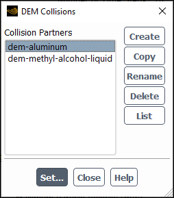
Controls
- Collision Partners
contains a list from which you can select one or more collision partners in order to set, create, copy, rename, delete, or list.
- Create
creates a new collision partner and opens the Create Collision Partner Dialog Box, in which you can enter the collision partner name.
- Copy
creates a new injection with the same properties as the selected collision partner and opens the Copy Collision Partner Dialog Box.
- Rename
allows you to change the name of the collision partner. It opens the Copy Collision Partner Dialog Box.
- Delete
deletes the collision partner selected in the Collision Partners list.
- List
lists the collision partners with their corresponding laws.
- Set...
opens the DEM Collision Settings Dialog Box for the collision partner selected in the Collision Partners list.
The Create Collision Partner dialog box allows you to specify the name of the collision partner.
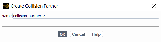
Controls
- Name
is the name of the collision partner being created.
The Copy Collision Partner dialog box allows you to copy the selected collision partner.
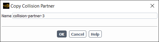
Controls
- Name
is the name of the new collision partner copied from the selected partner.
The Rename Collision Partner dialog box allows you to rename the selected collision partner.

Controls
- Name
is the new name of the collision partner selected in the list.
The DEM Collision Settings dialog box allows you to specify the collision laws of the collision partners.
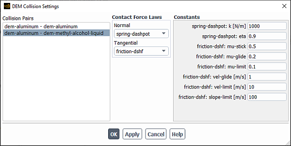
Controls
- Collision Pair
contains the list of created collision partners.
- Contact Force Laws
is where you will define the collisions laws.
- Normal
allows you to choose between spring, spring-dashpot, hertzian, and hertzian-dashpot. You can also choose none if you do not want to include a contact force.
- Tangential
allows you to choose between the friction-dhsf and friction-dshf-rolling force laws. You can also exclude a force law, in which case you would select none.
- Constants
contains the list of contact force constants. Depending on the contact force law in effect, different constants will be visible.
The Solidification and Melting dialog box allows you to set parameters related to the solidification/melting model. See Modeling Solidification and Melting for details about the items below.
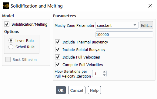
Controls
- Model
contains the option for turning on the model.
- Solidification/Melting
enables/disables the modeling of solidification and/or melting.
- Options
gives you the option of selecting one of two model rules.
- Lever Rule
allows you to use the Lever rule (Equation 15–14 in the Theory Guide).
- Scheil Rule
allows you to use the Scheil rule (Equation 15–18 in the Theory Guide). If you select Scheil Rule, then you can enable Back Diffusion. Enter either a constant or a user-defined function to specify the value of the Back Diffusion Parameter, used in Equation 15–19 to Equation 15–21 in the Theory Guide. Refer to
DEFINE_SOLIDIFICATION_PARAMSof the Fluent Customization Manual for detailed information about the user-defined function.
- Parameters
contains parameters related to the solidification/melting model.
- Mushy Zone Constant
sets the value of
 in Equation 15–6 in the Theory Guide.
- Include Thermal Buoyancy
includes the gravitational force due to the variation of density with temperature. Refer to Thermal and Solutal Buoyancy in the Theory Guide for more information.
Note: This option is available only when solidification is modeled with species transport.
- Include Solutal Buoyancy
includes the gravitational force due to the variation of density with the change in the species composition of the melt. Refer to Thermal and Solutal Buoyancy in the Theory Guide for more information.
Note: This option is available only when solidification is modeled with species transport.
- Include Pull Velocities
includes pull velocities in the model, as described in Momentum Equations and Pull Velocity for Continuous Casting in the Theory Guide.
- Compute Pull Velocities
enables the calculation of pull velocities based on the specified velocity boundary conditions, as described in Pull Velocity for Continuous Casting in the Theory Guide. This option appears when Include Pull Velocities is turned on.
- Flow Iterations per Pull Velocity Iteration
specifies the number of times the pull velocity equations will be solved after each iteration of the solver. This option appears when Compute Pull Velocities is turned on.
The Acoustics Models dialog box allows you to set parameters related to the acoustics model. See Predicting Aerodynamically Generated Noise for details about the items below.
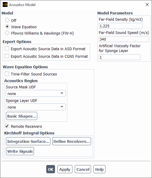
Controls
- Model
contains the option for turning on the acoustics model.
- Off
disables the acoustics model.
- Wave Equation
enables the wave equation model. See Using the Acoustics Wave Equation Model for details.
- Ffowcs-Williams & Hawkings
enables the Ffowcs Williams and Hawkings (FW-H) acoustics model. See Postprocessing the FW-H Acoustics Model Data for details.
- Broadband Noise Sources
enables the broadband noise acoustics model. See Using the Broadband Noise Source Models for details.
- Export Options
contains the parameters related to exporting acoustics data.
- Export Acoustic Source Data in ASD Format
enables/disables the saving of source data files in ASD format.
- Export Acoustic Source Data in CGNS Format
enables/disables the saving of source data files in CGNS format.
- Compute Acoustics Signals Simultaneously
enables "on-the-fly" calculation of sound. When this option is chosen, the Ansys Fluent console window will print a message at the end of each time step indicating that the sound pressure signals have been computed (for example,
Extracting sound signals at x receiver locations..., wherexis the number of receivers you specified). Enabling this option instructs Ansys Fluent to compute sound pressure signals at the end of each time step, which will slightly increase the computation time.
- Wave Equation Options
contains options for the wave equation.
- Time-Filter Sounds Sources
enables/disables the filtering of sounds sources.
- Source Mask UDF
Specifies a UDF for the source mask.
- Sponge Layer UDF
Specifies a UDF for the sponge layer.
- Basic Shapes...
opens the Basic Shapes Dialog Box, which allows you to specify shapes for source mask and sponge layer geometry.
- Remote Receivers
enables/disables the Kirchhoff integral model.
- Integration Surface…
selects the integration surface for the Kirchhoff model.
- Define Receivers…
opens the Acoustic Receivers Dialog Box, which allows you to specify the location of the receivers.
- Write Signals
writes the computed receiver signals to the ASCII files.
- Ffowcs-Williams & Hawkings Options
contains the Convective Effects option, which should be enabled for all cases dealing with external flows around bodies. When this option is enabled, you will need to specify the proper Free Stream Velocity and Free Stream Direction.
- Define Sources...
opens the Acoustic Sources Dialog Box, which allows you to specify the acoustics sources.
- Define Receivers...
opens the Acoustic Receivers Dialog Box, which allows you to specify the location of the receivers.
- Model Constants
contains parameters related to the acoustics model.
- Far-Field Density
sets the value of the far-field fluid density (
 in Equation 11–1 in the Theory Guide).
- Far-Field Sound Speed
sets the speed of the sound at the far-field (
 in Equation 11–5 and Equation 11–6 in the Theory Guide).
- Artificial Viscosity Factor for Sponge Layer
Set the Artificial Viscosity Factor for Sponge Layer.
- Free Stream Velocity
is available when the Convective Effects option for the Ffowcs-Williams & Hawkings model is enabled.
- Free Stream Direction
is available when the Convective Effects option for the Ffowcs-Williams & Hawkings model is enabled.
- Reference Acoustic Pressure
is used to calculate the sound pressure level in dB.
- Reference Acoustic Power
is used to non-dimensionalize the acoustic power, giving the sound pressure level in dB (see Fast Fourier Transform (FFT) Postprocessing). This parameter is equal to
 W for airborne sound and
  W
for underwater sound.
W
for underwater sound.- Reference Acoustic Intensity
is defined as
 ,
although this quantity is not currently used by Ansys Fluent.
,
although this quantity is not currently used by Ansys Fluent.- Source Correlation Length
is required when sound is to be computed using a 2D flow result. The FW-H integrals will be evaluated over this length in the depthwise direction using the identical source data.
- Number of Realizations
is the number of times the noise source terms will be computed through the generation of stochastic turbulent velocity field.
- Number of Fourier Modes
is the number of terms in the Fourier summation from which the turbulent velocity field and its derivatives are computed.
- Number of Time Steps Per Revolution
is available only for steady-state cases that have a single moving reference frame. Here you will specify the number of equivalent time steps that it will take for the rotating zone to complete one revolution.
- Number of Revolutions
is available only for steady-state cases that have a single moving reference frame. Here you will specify the number of revolutions that will be simulated in the model.
- Apply
saves the acoustics model settings.
The Acoustic Sources dialog box allows you to specify the acoustics sources. See Using the Ffowcs Williams and Hawkings Acoustics Model for details about the items below.
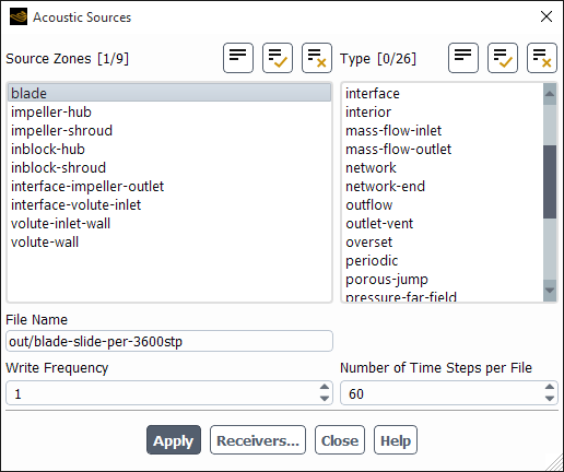
Controls
- Source Zones
contains a list of zones from which you can select one or more emission (source) surfaces.
- Type
contains a list of all possible types of zones from which you can select one or more types of the available zones. If you select an available type of zone, the relevant zones will then be selected in the Source Zones list. If you specify any valid interior zones as source surfaces, the Interior Cell Zone Selection Dialog Box will appear.
- File Name
is used to give the names of the source data files (for example,
acoustic_example_xxxx.asd, wherexxxxis the global time-step index of the transient solution) and an index file (for example,acoustic_example.index) that will store the information associated with the source data.- Write Frequency
allows you to control how often the source data will be written. This will enable you to save disk space if the time-step size used in the transient flow simulation is smaller than necessary to resolve the sound frequency you are attempting to predict.
- Number of Time Steps per File
allows you to write the source data to multiple files, each containing the source data for a number of time steps specified by you.
- Receivers...
opens the Acoustic Receivers Dialog Box, which allows you to specify the location of the receivers.
The Acoustic Receivers dialog box allows you to specify the location of the acoustic receivers. See Using the Ffowcs Williams and Hawkings Acoustics Model for details about the items below.
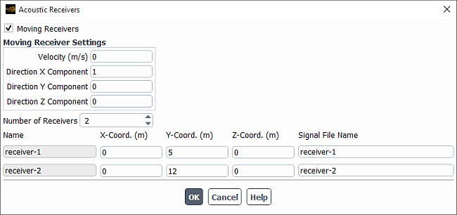
Controls
- Moving Receivers
allows you to specify the locations of the moving receivers.
- Moving Receiver Settings
allows you to specify the Velocity and the Direction of the moving receivers.
- Number of Receivers
allows you to specify the total number of receivers for which you want to compute sound.
- Name
shows the name of the receiver. If you edit the field, the new name will take effect after you click the button.
- X-Coord., Y-Coord., Z-Coord.
specifies the coordinates for each receiver. Note that because Ansys Fluent’s acoustics model is ideally suited for far-field noise prediction, the receiver locations you define should be at a reasonable distance from the sources of sound (that is, the selected acoustic surface), and can fall outside of the computational domain if needed.
- Signal File Name
specifies the name of the file used to store sound pressure signals for the corresponding receivers. By default, the files will be named
receiver-1.dat.h5,receiver-2.dat.h5, and so on.
The Basic Shapes dialog box allows you to select shapes for use as source mask and sponge layer geometry.
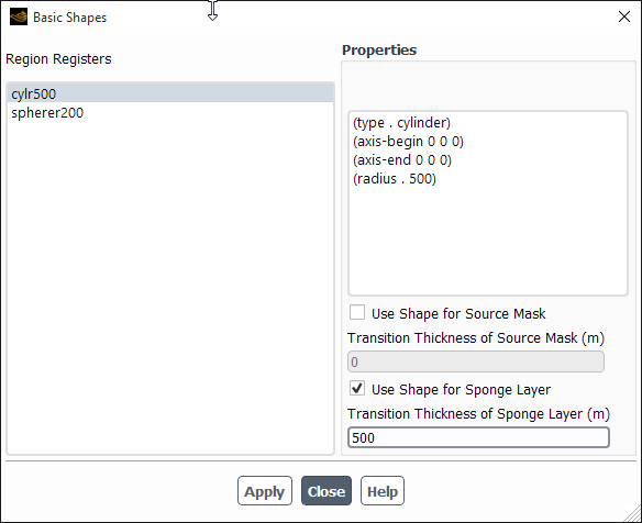
Controls
- Region Registers
contains a list of all registers which have been created for use as geometric shapes.
- Properties
displays information about the selected region register.
- Use Shape for Source Mask
enables/disables the use of the selected region register as a source mask.
- Transition Thickness of Source Mask
Specifies transition thickness of source mask.
- Use Shape for Sponge Layer
enables/disables the use of the selected region register as a sponge layer.
- Transition Thickness of Sponge Layer
Specifies transition thickness of sponge layer.
The Integration Surface Dialog Box displays a list of all currently available surfaces. With the current implementation only one surface can be selected in the list and used for the integration..
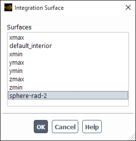
Controls
- Surfaces
contains a list of all surfaces that can be used as an integration surface.
The Interior Cell Zone Selection dialog box allows you to specify the acoustics sources. See Specifying Source Surfaces for details about the items below.
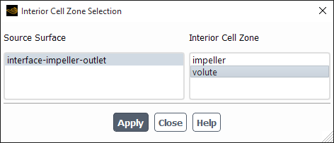
Controls
- Source Surface
displays the selected interior surface.
- Interior Cell Zone
contains a list of two interior cell zones, from which you will select the zone that is occupied by the quadrupole sources.
The Structural Model dialog box allows you to enable structural model calculations as part of an intrinsic fluid-structure interaction (FSI) problem. For details, see Modeling Fluid-Structure Interaction (FSI) Within Fluent.
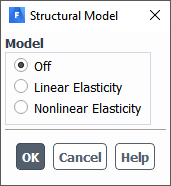
Controls
- Model
indicates which model, if any, is used for the structural model calculations.
- Off
disables structural model calculations.
- Linear Elasticity
enables structural calculations for the solid cell zone such that the internal load is linearly proportional to the nodal displacement, and the structural stiffness matrix remains constant. This model is appropriate when the stress loading does not exceed the yield strength of the solid material.
- Nonlinear Elasticity
enables you to model geometrically nonlinear elasticity, in order to simulate large deformation in solid cell zones.
- Options
allows you access to fluid-structural interaction options.
- Thermal Effects
enables you to simulate the effects of thermal loads on solid structure deformation.
The Eulerian Wall Film dialog box allows you to set various model and solution method controls for the Eulerian Wall Film model. For more information, see Modeling Eulerian Wall Films.
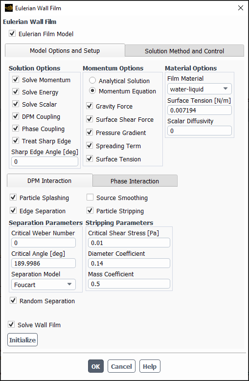
Controls
- Eulerian Wall Film
enables/disables the use of the Eulerian Wall Film model in the calculations.
- Model Options and Setup
contains controls for specific solution, discrete phase model (DPM), and material options for the Eulerian Wall Film model.
- Solution Options
includes options for enabling/disabling the momentum equation and DPM calculations.
- Solve Momentum
specifies whether film velocity is solved for the wall film. When the option is disabled, film velocity is fixed at the existing values. When the option is enabled, you can choose to solve film velocity using options in the Momentum Options group box.
- Solve Energy
allows the energy equation (see Equation 17–3 in the Fluent Theory Guide) to be solved.
- Solve Scalar
allows the passive scalar equation (see Equation 17–38 in the Fluent Theory Guide) to be solved. Once you enable this option, you can set Scalar Diffusivity in the Material Options group box.
- DPM Coupling
enables the interaction of discrete phase particles with the film model (see DPM Collection in the Fluent Theory Guide). When this option is enabled, you can adjust the DPM coupling settings in the DPM Interaction tab. This option is only available when the DPM model is enabled.
- Phase Coupling
allows you to account for phase changes between the film material (liquid) and the gas species (vapor) (see Coupling of Wall Film with Mixture Species Transport in the Fluent Theory Guide) and compute the secondary phase collection efficiency on a wall surface. When this option is enabled, you can adjust the phase coupling settings in the Phase Interaction tab. This option is only available when the Eulerian or Mixture (with Slip Velocity) multiphase model or the species model is enabled.
- Treat Sharp Edge
allows you to set the Sharp Edge Angle when handling the effects of sharp edges alongside the wall film.
- Momentum Options
is a group box where you can select from the following solution methods. This item is available when the Solve Momentum option is enabled.
- Analytical Solution
applies film velocity computed from the external flow shear and gravity as described in Obtaining Film Velocity Without Solving the Momentum Equations in the Fluent Theory Guide.
- Momentum Equation
enables the solution of the film momentum equation (see Equation 17–2). You can select the following terms for inclusion in the calculation:
- Gravity Force
is the second term on the right hand side of Equation 17–2, and is responsible for accelerating the film in the direction of gravity component that is parallel to the wall.
- Surface Shear Force
is the third term on the right hand side of Equation 17–2, and is responsible for accelerating the film in the direction of the external flow.
- Pressure Gradient
is the first term on the right hand side of Equation 17–2, and is the term accelerating the film in the direction opposing the gradient in external pressure. For example, if a film on the surface of a wing is being modeled and there is a high pressure region at the leading edge with low pressure on the top of the wing, this term will tend to move a uniform film towards the low pressure region on the top of the wing.
- Spreading Term
is the
 term on the right hand side of Equation 17–2, and is responsible for spreading. This term
will accelerate the flow in the direction opposing the gradient in height, moving the
film towards regions of lower thickness. This term becomes available only when both
Pressure Gradient and Gravity Term are
selected.
term on the right hand side of Equation 17–2, and is responsible for spreading. This term
will accelerate the flow in the direction opposing the gradient in height, moving the
film towards regions of lower thickness. This term becomes available only when both
Pressure Gradient and Gravity Term are
selected. - Surface Tension
is the
 term on the right hand side of Equation 17–2. This term becomes available only when
Pressure Gradient is selected.
term on the right hand side of Equation 17–2. This term becomes available only when
Pressure Gradient is selected.
- Material Options
allows you to apply material properties to the wall film model.
- Film Material
is the material assigned to the wall film.
- Surface Tension
is the surface tension for the designated wall film material. This item is available only when the Solve Momentum option is enabled in the Solution Options group box.
- Scalar Diffusivity
is the diffusivity of the scalar being modeled for the designated wall film material. This item is available only when the Solve Momentum option is enabled in the Solution Options group box.
- DPM Interaction
tab defines the interaction between the discrete phase and the film (see DPM Collection in the Fluent Theory Guide). this tab is available when DPM Coupling is enabled in the Solution Options group box.
- Particle Splashing
allows you to account for splashing of the wall film particles. When this option is enabled, you can specify splashing options in the Wall Film tab of the Wall dialog box. For details, see Setting Eulerian Wall Film Boundary, Initial, and Source Term Conditions.
- Source Smoothing
When enabled, smoothing is applied to the discrete phase impingement source terms to reduce the impact of spotty source distributions.
- Edge Separation
allows you to specify the following Separation Parameters:
- Critical Weber Number
is the critical value for the Weber number.
- Critical Angle
is the critical angle, θ, that separation occurs.
- Separation Model
allows you to specify one of three different models to calculate the number and diameter of the shed particle stream at an edge once separation occurs. Available models include: Foucart (the default, see Foucart Separation in the Theory Guide), O'Rourke (see O’Rourke Separation), and Friedrich (see Friedrich Separation).
- Random Separation
allows the random selection of the locations at which the newly spawn particles are injected (due to film separation) along the edge at which the separation takes place.
- Particle Stripping
allows you to set the below DPM Stripping Parameters. For details about these settings, see Film Separation in the Fluent Theory Guide.
- Critical Shear Stress
is the critical value of the shear stress on the face where liquid film exists, which, when exceeded, causes mass to be taken from the film.
- Diameter Coefficient
is the value of
 used in Equation 17–20 in the Theory Guide.
- Mass Coefficient
is the value of
 used in Equation 17–21 in the Theory Guide.
- Phase Interaction
tab allows you to set secondary phase accretion options (see Secondary Phase Accretion in the Theory Guide). The tab is available when Phase Coupling is enabled in the Solution Options group box.
- Phase Change
allows you to account for phase changes between the film material (liquid) and the gas species (vapor). When this option is selected, you can specify the phase change parameters on the selected film wall boundaries in the Wall Film tab of the Wall Dialog Box. (See Coupling of Wall Film with Mixture Species Transport in the Fluent Theory Guide). This option is only available when the species model is enabled.
- Film Vapor Material
is the material assigned to the wall film vapor.
- Phase Accretion
(available when the Eulerian Multiphase or Mixture (with Slip Velocity) model is enabled) allows for the interaction of the wall film with a secondary phase in a multiphase flow. Once enabled, you can set the Phase Accretion Parameters (see Secondary Phase Accretion in the Theory Guide).
- Phase Concentration
is the value of
 used in Equation 17–24 in the Theory Guide.
- Phase Velocity
is the value of
 used in Equation 17–24 in the Theory Guide.
- Solve Wall Film
allows you to skip the wall film solution during the gas phase solution, but keep the variables and setup active.
- Initialize
allows you to initialize the wall film variables and prepare the solver for the solution procedure. The film cannot be solved without first initializing the wall film model.
- Solution Method and Control
contains controls for temporal or spatial discretization as well as wall film thickness for the Eulerian Wall Film model.
- Discretization
allows you to set the temporal or spatial discretization methods.
- Time
allows you to specify the temporal discretization methods. Available options include: First Order Explicit, High Order Explicit, First Order Implicit, or Second Order Implicit.
- Continuity
allows you to specify the spatial discretization methods for continuity. Available options include: First Order Upwind, or Second Order Upwind.
- Momentum
allows you to specify the spatial discretization methods for momentum. Available options include: First Order Upwind, or Second Order Upwind.
- Energy
allows you to specify the spatial discretization methods for energy. Available options include: First Order Upwind, or Second Order Upwind.
- Thickness Control
allows you to specify Maximum Thickness.
- Continuity and Momentum Coupling
is a group box where you can specify the following coupling solution inputs. This item appears only when Solve Momentum is selected in the Model Options and Setup tab. For more information about these options, see Coupled Solution Approach in the Fluent Theory Guide.
- Coupled Solution
enables the coupled solution approach.
- Curvature Smoothing
applies smoothing to the film variables. When this option is enabled, you can specify Smoothing Level and Smoothing Factor. This item appears only when Surface Tension is selected in the Model Options and Setup tab.
- Time Marching and Time Step Control
allows you to set the number of sub-steps that the film model will take between time steps from the main solver. For example, if the flow time step is 0.001 seconds and the number of time steps is set to 10 in the film model, the film model will take 10 time steps of 0.0001 so that the film time and the flow time match at the end of the solution step. For implicit time stepping, the film model will take 5 additional sub iterations per implicit step, stopping the sub-step when the film residual drops below the value set in the Sub-Iteration Stop option.
- Adaptive Time Stepping
(steady-state flow) enables the adaptive time stepping method to determine the film time step size (
 ) using the maximum Courant number and the initial time step (see
Steady Flow in the Theory Guide).
) using the maximum Courant number and the initial time step (see
Steady Flow in the Theory Guide).- Max. Courant Number
is the maximum value of the Courant number used to compute the film time step.
- Initial Time Step
is an initial value for the time step used to compute the film time step.
- Time-Step
(steady-state flow; default) is the user-specified size of the time step,
 (see Steady Flow in the Theory Guide).
- Per Flow Iterations
(transient flow) specifies the flow iteration interval at which the flow solution is called within each flow time step. The film solution is always called at the first flow iteration.
- Sub-Time Steps
(transient flow) is
 used in Equation 17–52 in the Theory Guide.
- Sub-Time Report Interval
(transient flow) specifies the number of iterations between the wall film solution reports.
- Sub-Iterations
(available when either First Order Implicit or Second Order Implicit are enabled for Time under Discretization) is the number of additional sub iterations per implicit step.
- Sub-Iteration Stop
(available when either First Order Implicit or Second Order Implicit are enabled for Time under Discretization) is the point at which the sub iterations stop (when the film residual drops below this value).
- Sub-Iter Report Interval
(implicit time discretization calculation) specifies the number of sub-iterations between the wall film solution reports.
- DPM Control
(available when DPM Coupling is enabled in the Model Options and Setup tab) allows you to specify DPM-specific discretization.
- Film Steps per DPM Step
allows you to set how often the DPM phase is calculated for the film.
The Battery Model dialog box allows to set parameters related to thermal and electrochemical behavior of a single battery cell or a battery pack.
Controls
- Enable Battery Model
enables/disables the battery modeling.
- Model Options
tab allows you to select the solution method and E-chemistry model, and specify general battery model settings. See Specifying Battery Model Options for detailed information about available models and settings.
- Conductive Zones
tab allows you to select zones for the active, tab and busbar components. See Specifying Conductive Zones for detailed information about available settings.
- Electric Contacts
tab allows you to define the contact surface and external connectors. See Specifying Electric Contacts for detailed information about available settings.
- Model Parameters
tab allows you to specify the parameters to be used for solving the model equations. See Specifying Battery Model Parameters for detailed information about available controls.
- UDF
tab allows you to hook your user-defined functions. See Hooking User-Defined Functions for detailed information about this tab.
- Advanced Options
tab allows you to quickly check the selected electrochemical submodel behavior in a standalone mode, and also to use various advanced capabilities. See Specifying Advanced Options for more information.
initializes the battery model only. See Initializing the Battery Model for more information.
restores the last saved settings for all tabs.
- Apply
saves the specified values and options for the selected model.
The Standalone Echem Model dialog box enables you to:
Perform a quick analysis of your electrochemical model by simulating it in a standalone mode
Predict the battery aging process during a large number of electric load cycles in the standalone mode
For a full description of available controls, see:
The Potential/Electrochemistry dialog box allows you to set parameters related to the electric potential field or electrochemistry models (Li-ion battery model or electrolysis and H2 pump model) in your simulation. See Setting Up the Electric Potential Model, Setting Up the Lithium-ion Battery Model, and Setting the Electrolysis and H2 Pump Model for details.
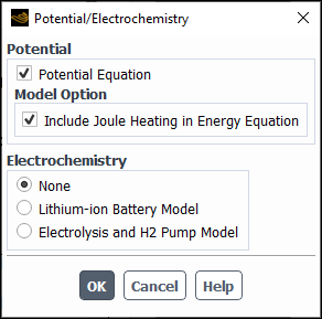
Controls
- Potential
contains controls related to modeling of the electric potential field.
- Potential Equation
enables/disables the simulation of the electric potential field in the model.
- Model Option
allows you to enable/disable the Include Joule Heating in Energy Equation option. This option appears only if the energy equation is enabled.
- Electrochemistry
contains the following electrochemistry options:
- None
no electrochemistry is involved in the simulation
- Lithium-ion Battery Model
allows you to enables the Lithium-ion Battery model and specify related parameters as described in Simulating the Lithium-ion Battery. This option is available only when the Potential Equation is enabled.
- Electrolysis and H2 Pump Model
allows you to enables the electrolysis and H2 pump model and specify related parameters as described in Setting the Electrolysis and H2 Pump Model. This option is available only when the Potential Equation is enabled.