


For background information about the VOF model and the limitations that apply, refer to Overview of the VOF Model in the Theory Guide.
This section is organized as follows:
- 26.3.1. Solving Steady-State VOF Problems
- 26.3.2. Guidelines for Using the Multiphase Pseudo Time Method
- 26.3.3. Including Coupled Level Set with the VOF Model
- 26.3.4. Mesh Adaption with the VOF Model
- 26.3.5. Modeling Open Channel Flows
- 26.3.6. Modeling Open Channel Wave Boundary Conditions
- 26.3.7. Recommendations for Open Channel Initialization
- 26.3.8. Numerical Beach Treatment for Open Channels
- 26.3.9. Defining the Phases for the VOF Model
- 26.3.10. Defining Phase Interaction Terms
- 26.3.11. Setting Time-Dependent Parameters for the Explicit Volume Fraction Formulation
- 26.3.12. Modeling Solidification/Melting
- 26.3.13. Using the VOF-to-DPM Model Transition for Dispersion of Liquid in Gas
- 26.3.14. Using the DPM-to-VOF Model Transition
For steady-state VOF problems, Ansys Fluent automatically selects Global Time Step from the Pseudo Time Method list in the Solution Methods task page and enables the Coupled pressure-velocity coupling scheme, in order to provide better stability and faster convergence. For more information about pseudo time method solutions, see Performing Calculations with a Pseudo Time Method.
When using a Pseudo Time Method in multiphase applications, follow the guidelines provided below:
For the fixed (User-Specified) time step method, you must provide a suitable pseudo time step size to the solver. You can use the Automatic time step method to estimate the pseudo time step size for the simulation. This can be done by setting the Verbosity to 1 and simulating your case for a few iterations. The pseudo time step size will be printed in the Fluent console.
For the Automatic time step method, decreasing the Time Scale Factor to a lower value (about 0.3) will provide better solution stability.
Sometimes, for stiff flow problems, convergence may not be achieved when using the Automatic time step method. In such cases, consider switching to the fixed (User-Specified) time step method instead.
For steady-state problems, you should never evaluate convergence based on residuals alone. To better judge convergence, you should also monitor appropriate field variables at a particular location until the value stops changing.
The Coupled with Volume Fractions option is recommended for open channel flow applications.
When using the VOF formulation, you can couple the level set method with it to help overcome some limitations that exist in the interface tracking method of the VOF model and the level set method. To use the coupled level set method with VOF, perform the following:
Open the Multiphase Model dialog box.
 Setup →
  Models →
  Multiphase → Edit...
In the Model group box (Models tab), enable Volume of Fluid.
In the Hybrid Models group box, enable Coupled Level Set + VOF (see Figure 26.1: Multiphase Model Dialog Box for the VOF Model).
(optional) In some cases, spurious currents can arise from the application of the surface tension force in the momentum equation. In these cases you can use the
/define/models/multiphase/coupled-level-settext command to use a revised formulation of the surface tension force that weights the force towards the heavier phase in the interface cells. You can choose fromnone(the default),density-correction, andheaviside-correction.
After the Coupled Level Set + VOF option is enabled, proceed as you normally would when setting up the VOF model (described in Setting Up the VOF Model). For theoretical information, refer to Coupled Level-Set and VOF Model in the Fluent Theory Guide.
Note: When using the Coupled Level Set + VOF option, the recommended scheme is the geo-reconstruct scheme (see The Geometric Reconstruction Scheme in the Fluent Theory Guide).
For additional limitations associated with the level set method, see Limitations in the Fluent Theory Guide.
Normally, zero flux of the level set function is set as the default for the boundary conditions. Due to the geometrical re-initialization procedure at each time step, the boundary conditions shall not have any significant effect on the results. For more information, see Re-initialization of the Level-set Function via the Geometrical Method.
It may be useful to refine and/or coarsen the mesh of your VOF simulation based on the volume fraction of the phases. For information about mesh adaption, see Adapting the Mesh. Note that an easy way to define the settings in the Manual Mesh Adaption or Automatic Mesh Adaption dialog box for VOF simulations is to use the Predefined Criteria drop-down list, as described in VOF Adaption. This list allows you to select from commonly used criteria for adapting the mesh; the Multiphase... submenu provides an option for standard VOF cases, as well as options for straightforward or more complex cases that use the VOF-to-DPM model transition mechanism.
Using the VOF formulation, open channel flows can be modeled in Ansys Fluent. To start using the open channel flow boundary condition, perform the following:
Enable Gravity and set the gravitational acceleration fields.
Setup → General Gravity → On
Enable the volume of fluid model.
Open the Multiphase Model dialog box.
Setup → Models →
Multiphase → Edit...
In the Model group box (Models tab), enable Volume of Fluid.
In the Formulation group box, select either Implicit or Explicit.
In the VOF Sub-Models tab, select Open Channel Flow.
Note: The default VOF formulation is set to Implicit after enabling the Open Channel Flow option. This is done to allow the use of larger time step sizes for such applications.
In order to set specific parameters for a particular boundary for open channel flows, enable the Open Channel option in the Multiphase tab of the corresponding boundary condition dialog box. Table 26.10: Open Channel Boundary Parameters for the VOF Model summarizes the types of boundaries available to the open channel flow boundary condition, and the additional parameters needed to model open channel flow. For more information on setting boundary condition parameters, see Cell Zone and Boundary Conditions.
Table 26.10: Open Channel Boundary Parameters for the VOF Model
| Boundary Type | Parameter |
|---|---|
| pressure inlet | Inlet Group ID; Secondary Phase for Inlet; Flow Specification Method; Free Surface Level, Bottom Level; Velocity Magnitude |
| pressure outlet | Outlet Group ID; Pressure Specification Method; Free Surface Level; Bottom Level |
| mass-flow inlet | Inlet Group ID; Secondary Phase for Inlet; Free Surface Level; Bottom Level; Mass Flow Rates for the Phases |
| velocity inlet | Secondary Phase for Inlet; Free Surface Level, Averaged Velocity Inputs/Segregated Velocity Inputs (Available with Open Channel Wave Boundary Condition) |
| outflow | Flow Rate Weighting |
Further details are provided in the following sections:
- 26.3.5.1. Defining Inlet Groups
- 26.3.5.2. Defining Outlet Groups
- 26.3.5.3. Setting the Inlet Group
- 26.3.5.4. Setting the Outlet Group
- 26.3.5.5. Determining the Free Surface Level
- 26.3.5.6. Determining the Bottom Level
- 26.3.5.7. Specifying the Total Height
- 26.3.5.8. Determining the Velocity Magnitude
- 26.3.5.9. Determining the Secondary Phase for the Inlet
- 26.3.5.10. Determining the Secondary Phase for the Outlet
- 26.3.5.11. Choosing the Pressure Specification Method
- 26.3.5.12. Choosing the Density Interpolation Method
- 26.3.5.13. Open Channel Flow Compatibility with Velocity Inlet
- 26.3.5.14. Limitations
- 26.3.5.15. Recommendations for Setting Up an Open Channel Flow Problem
Open channel systems involve the flowing fluid (the secondary phase) and the fluid above it (the primary phase).
If both phases enter through the separate inlets (for example, inlet-phase2 and inlet-phase1), these two inlets form an inlet group. This inlet group is recognized
by the parameter Inlet Group ID, which will be
same for both the inlets that make up the inlet group. On the other
hand, if both the phases enter through the same inlet (for example, inlet-combined), then the inlet itself represents the
inlet group.
Important: In three-phase flows, only one secondary phase is allowed to pass through one inlet group.
Outlet-groups can be defined in the same manner as the inlet groups.
Important: In three-phase flows, the outlet should represent the outlet group, that is, separate outlets for each phase are not recommended in three-phase flows.
For pressure inlets and mass-flow inlets, the Inlet Group ID is used to identify the different inlets that are part of the same inlet group. For instance, when both phases enter through the same inlet (single face zone), then those phases are part of one inlet group and you would set the Inlet Group ID to 1 for that inlet (or inlet group).
In the case where the same inlet group has separate inlets (different face zones) for each phase, then the Inlet Group ID will be the same for each inlet of that group.
When specifying the inlet group, use the following guidelines:
Since the Inlet Group ID is used to identify the inlets of the same inlet group, general information such as Free Surface Level, Bottom Level, or the mass flow rate for each phase should be the same for each inlet of the same inlet group.
You should specify a different Inlet Group ID for each distinct inlet group.
For example, consider the case of two inlet groups for a particular problem. The first inlet group consists of water and air entering through the same inlet (a single face zone). In this case, you would specify an inlet group ID of 1 for that inlet (or inlet group). The second inlet group consists of oil and air entering through the same inlet group, but each uses a different inlet (
oil-inletandair-inlet) for each phase. In this case, you would specify the same Inlet Group ID of 2 for both of the inlets that belong to the inlet group.
For pressure outlet boundaries, the Outlet Group ID is used to identify the different outlets that are part of the same outlet group. For instance, when both phases enter through the same outlet (single face zone), then those phases are part of one outlet group and you would set the Outlet Group ID to 1 for that outlet (or outlet group).
In the case where the same outlet group has separate outlets (different face zones) for each phase, then the Outlet Group ID will be the same for each outlet of that group.
When specifying the outlet group, use the following guidelines:
Since the Outlet Group ID is used to identify the outlets of the same outlet group, general information such as Free Surface Level or Bottom Level should be the same for each outlet of the same outlet group.
You should specify a different Outlet Group ID for each distinct outlet group.
For example, consider the case of two outlet groups for a particular problem. The first outlet group consists of water and air exiting from the same outlet (a single face zone). In this case, you would specify an outlet number of 1 for that outlet (or outlet group). The second outlet group consists of oil and air exiting through the same outlet group, but each uses a different outlet (
oil-outletandair-outlet) for each phase. In this case, you would specify the same Outlet Group ID of 2 for both of the outlets that belong to the outlet group.
Important: For three-phase flows, when all the phases are leaving through the same outlet, the outlet should consist only of a single face zone.
For the appropriate boundary, you need to specify the Free Surface Level
value. This parameter is available for all relevant boundaries, including pressure outlet,
mass-flow inlet, and pressure inlet. The Free Surface Level, is represented by  in Equation 14–42 in the Theory Guide.
 | (26–10) |
where  is the position vector of any
point on the free surface, and
is the position vector of any
point on the free surface, and  is the unit vector in the direction of
the force of gravity. Here a horizontal free surface that is normal
to the direction of gravity is assumed.
is the unit vector in the direction of
the force of gravity. Here a horizontal free surface that is normal
to the direction of gravity is assumed.
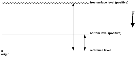
We can simply calculate the free surface level in two steps:
Determine the absolute value of height from the free surface to the origin in the direction of gravity.
Apply the correct sign based on whether the free surface level is above or below the origin.
If the liquid’s free surface level lies above the origin, then the Free Surface Level is positive (see Figure 26.27: Determining the Free Surface Level and the Bottom Level). Likewise, if the liquid’s free surface level lies below the origin, then the Free Surface Level is negative.
You can also specify a transient profiles for a Free Surface Level for the relevant open channel boundaries as shown in the example below:
/*********************************************************************
Example UDF that demonstrates transient profile for free surface level
**********************************************************************/

#include "udf.h"

#define H 1.5   /* Original Free surface level */
#define T0 0.2  /* Time */

DEFINE_TRANSIENT_PROFILE(fs_level, current_time)
{
    real level;
    if (current_time <= T0)
      level = H - current_time;
    else
      level = H - T0;

    return level;
}
For the appropriate boundary, you need to specify the Bottom Level value. This parameter is available for all relevant boundaries, including pressure outlet, mass-flow inlet, and pressure inlet. The Bottom Level, is represented by a relation similar to Equation 14–42 in the Theory Guide.
 | (26–11) |
where  is the position vector of any
point on the bottom of the channel, and
is the position vector of any
point on the bottom of the channel, and  is the unit vector of gravity.
Here we assume a horizontal free surface that is normal to the direction
of gravity.
is the unit vector of gravity.
Here we assume a horizontal free surface that is normal to the direction
of gravity.
We can simply calculate the bottom level in two steps:
Determine the absolute value of depth from the bottom level to the origin in the direction of gravity.
Apply the correct sign based on whether the bottom level is above or below the origin.
If the channel’s bottom lies above the origin, then the Bottom Level is positive (see Figure 26.27: Determining the Free Surface Level and the Bottom Level). Likewise, if the channel’s bottom lies below the origin, then the Bottom Level is negative.
You can also specify a transient profiles for a Bottom Level for the relevant open channel boundaries.
The total height, along with the velocity, is used as an option for describing the flow. The total height is given as
 | (26–12) |
where  is the velocity magnitude and
  is the gravity magnitude.
For pressure inlet boundaries, input for Velocity Magnitude is required to calculate the dynamic pressure being used in the total pressure calculation.
Note: The provided Velocity Magnitude is not applied to the boundary.
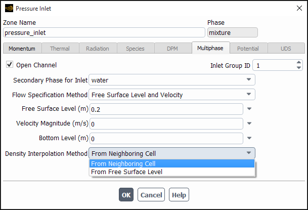
In the case of a flow with more than two phases, for pressure inlets and mass-flow inlets, you can select the desired secondary phase from the Secondary Phase for Inlet drop-down box.
Important: Note that only one secondary phase is allowed to pass through one inlet group.
Consider a problem involving a three-phase flow consisting of air as the primary phase, and oil and water as the secondary phases. Consider also that there are two inlet groups:
water and air
oil and air
For the former inlet group, you would choose water as the secondary phase. For the latter inlet group, you would choose oil as the secondary phase (as shown in Figure 26.28: Pressure Inlet for Open Channel Flow).
For a flow application with more than two phases, if you select Free Surface Level for the Pressure Specification Method (in the Pressure Outlet dialog box, Multiphase tab), you must also select the appropriate Secondary Phase for Level Specification and specify the Free Surface Level and Bottom Level. See Determining the Free Surface Level and Determining the Bottom Level for details about these parameters. For more information about the available pressure specification methods, refer to Pressure Outlet in the Fluent Theory Guide.
The hydrostatic pressure profile is imposed in the selected secondary phase that shares the interface with the primary phase. It is assumed that other secondary phases will not disturb the imposed pressure distribution.
For example, in a three-phase cavitating flow consisting of air, water, and vapor, the vapor is generated in the localized region adjacent to moving bodies. If the pressure outlet boundary is sufficiently far away from the cavitating region, then the hydrostatic assumption in the water phase that shares the interface with air can be safely imposed.
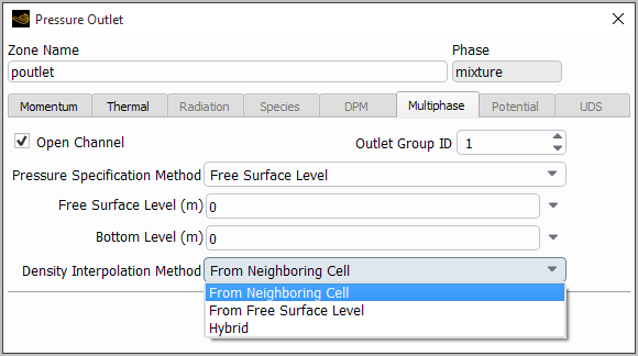
For a pressure outlet boundary, the outlet pressure can be specified in one of three ways:
by prescribing the free surface level, such as a hydrostatic pressure profile (available for two-phase flow only)
by specifying the constant pressure
by specifying the neighboring cell pressure
Note: You can also specify a hydrostatic pressure profile at the pressure outlet for axisymmetric open channel flow. However, there are certain limitations as noted in Limitations.
Important: This option is not available in the case of three-phase flows since the pressure on the boundary is taken from the neighboring cell.
For problems involving sub-critical flow, the following options exist for the Density Interpolation Method:
From Neighboring Cell is the default option, where the mixture density used in the hydrostatic profile is interpolated using the volume fraction calculated from the neighboring cell.
Note: In some cases, this method may cause free surface oscillation near the upstream boundaries. These oscillations are particularly visible in cases where boundaries are close to the object; or if the boundary has unstructured mesh near the free surface level. For such cases, it is recommended that you use the From Free Surface Level option under Density Interpolation Method.
From Free Surface Level where the mixture density used in the hydrostatic profile is interpolated from the volume fraction calculated from the free surface level.
Hybrid where the mixture density used in the hydrostatic profile is calculated either from the From Neighboring Cell or From Free Surface Level options, depending on the direction of flux. This method is only available at a pressure outlet.
For additional information, see the following sections:
Open channel flow compatibility with velocity inlet is provided in the framework of the open channel wave boundary condition, therefore, the Open Channel Wave BC option in the Figure 26.1: Multiphase Model Dialog Box for the VOF Model must be enabled first.
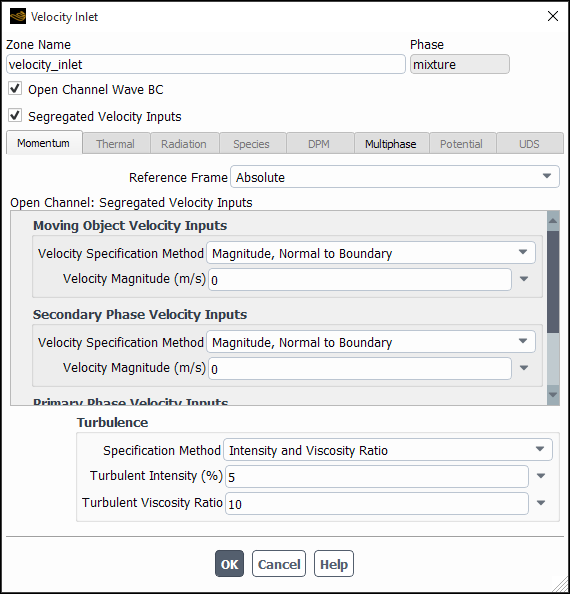
Velocity inlet compatibility allows you to use either averaged or segregated velocity inputs to moving obstacles, water and air, which is not possible using either the pressure inlet or mass-flow inlet boundary conditions.
Select the Open Channel Wave BC option in the Velocity Inlet dialog box. For detailed information about the velocity inputs, see Inputs at Velocity Inlet Boundaries.
You must specify (in the Multiphase tab of the Velocity Inlet dialog box):
Secondary phase for the inlet
Free surface level
The following list summarizes some issues and limitations associated with the open channel boundary condition.
The conservation of the Bernoulli integral does not provide the conservation of mass flow rate for the pressure boundary. In the case of a coarser mesh, there can be a significant difference in mass flow rate from the actual mass flow rate. For finer meshes, the mass flow rate comes closer to the actual value. So, for problems having constant mass flow rate, the mass flow rate boundary condition is a better option. The pressure boundary should be selected when steady and non-oscillating drag is the main objective.
Specifying the top boundary as the pressure outlet can sometimes lead to a divergent solution. This may be due to the corner singularity at the pressure boundary in the air region or due to the inability to specify local flow direction correctly if the air enters through the top locally.
Only the heavier phase should be selected as the secondary phase.
In the case of flows with more than two phases, only one secondary phase is allowed to enter through one inlet group (that is, the mixed inflow of different secondary phases is not allowed).
For axisymmetric flow, pressure and mass-flow inlets do not support open channel boundary conditions.
Open channel wave boundary conditions for velocity inlets do not support cases with axisymmetric flow.
Axisymmetric open channel flow is available for two phase flow and the pressure outlet boundary.
For axisymmetric open channel flow, the direction of gravity must be aligned with the direction of the axis.
The following list represents a list of recommendations for solving problems using the open channel flow boundary condition:
In the cases where the inlet group has a different inlet for each phase of fluid, then the parameter values (such as Free Surface Level, Bottom Level, and Mass Flow Rate) for each inlet should correspond to all other inlets that belong to the inlet group.
The solution begins with an estimated pressure profile at the outlet boundary.
In general, you can start the solution by assuming that the level of liquid at the outlet corresponds to the level of liquid at the inlet. The convergence and solution time is very dependent on the initial conditions. When the flow is completely subcritical (upstream and downstream), in marine applications for instance, the above approach is recommended.
If the final conditions of the flow can be predicted by other means, the solution time can be significantly reduced by using the proper boundary condition.
In the case of super-critical flow at the outlet, you can use the From Neighboring Cell option at the outlet, as it may provide better convergence.
The initialization procedure is very critical in the open channel analysis. Refer to Recommendations for Open Channel Initialization.
For the initial stability of the solution, a smaller time step size is recommended. You can increase the time step size once the solution becomes more stable.
For flows that do not make a transition from sub-critical to super-critical, or vice-versa, you can speed-up the solution calculation by specifying the frequency of Froude number updates during run time by setting the following text command:
solve→set→open-channel-controls.When prompted, set up the following parameter for steady-state flows:
/solve/set> open-channel-controls
Iteration interval for Froude number update [10]
When prompted, set up the following parameter for transient flows:
/solve/set> open-channel-controls
Time step interval for Froude number update [1]
For pure open channel flow applications, the inlet and outlet boundary conditions are controlled by the Froude number. In certain cases, it is possible to impose a hydrostatic profile at the outlet without any Froude number dependency. You can use the following text command:
solve→set→open-channel-controls.When prompted, set up the following parameter as shown below:
/solve/set> open-channel-controls
Use Froude number independent boundary condition at outlet? [no] yes
Relevant open channel inputs, along with the Froude number, can be reported using the following text command:
define→boundary-conditions→openchannel-threads.In the case of reverse flow, the pressure outlet boundary behaves as a pressure inlet, and the boundary-specific static pressure is taken as the Total Pressure. In this case, the static pressure is calculated from the total pressure. You can use the following text command to fix the boundary-specified static pressure, which helps to suppress reflections from the pressure boundary for certain cases:
solve→set→open-channel-controlsWhen prompted, set up the following parameter as shown below:
/solve/set> open-channel-controls
Use boundary specified static pressure for backflow? [no] yes
Open Channel + Translational Moving Reference Frame (MRF)
For high-speed moving hulls, it is generally recommended to ramp up the hull speed from zero to its actual speed for better stability. However, it has been observed that using pressure inlet or velocity inlet boundary conditions to mimic the hull speed causes many convergence issues. The alternative approach is to use a translational MRF with the following solution methodology:
Set the same speed for the whole domain as for the hull by using a transient profile for a gradual ramping. It is assumed that there is no bulk velocity of fluid.
Keep the wall boundary conditions stationary in the absolute reference frame.
Specify the inlet boundary condition using one of the following options:
Pressure-inlet with the following settings:
Select Relative to Adjacent Cell Zone for Reference Frame (Momentum tab of the Pressure Inlet dialog box).
Use the udf/profile option for Velocity Magnitude and hook the same transient profile of the hull speed (Multiphase tab of the Pressure Inlet dialog box.
Velocity Inlet with the following settings:
Select Absolute for Reference Frame (Momentum tab of the Velocity Inlet dialog box).
Set Velocity Magnitude to 0 m/s
In the Solution Initialization task page, set all velocity components to zero, and initialize the solution in the Absolute reference frame.
When modeling open channel wave boundary conditions, many of the variables that are used in open channel flow, also exist for open channel wave boundary conditions. You may have to refer to Modeling Open Channel Flows for information about some of the settings.
To use the open channel wave boundary condition, perform the following:
Enable Gravity and set the gravitational acceleration fields.
Setup → General Gravity → On
Enable the Volume of Fluid model in the Multiphase Model dialog box (Models tab).
Setup → Models →
Multiphase → Edit...
In the Formulation group box, select either Implicit or Explicit.
In the VOF Sub-Models group box, select Open Channel Wave BC.
In order to set specific parameters for a particular boundary for open channel wave boundaries, enable the Open Channel Wave BC option in the Velocity Inlet boundary condition dialog box (Figure 26.30: The Velocity Inlet for Open Channel Wave BC).
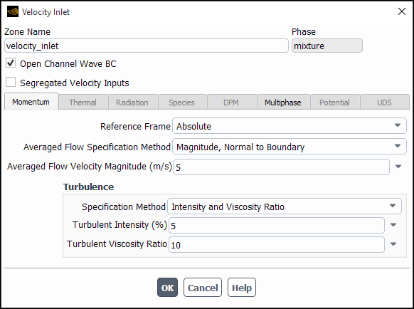
The default method is the Averaged Flow Specification Method, where inputs for the moving obstacle and water current are combined. There is no specific treatment for air velocity, which is assumed to be same as the averaged velocity.
Segregated Velocity Inputs
The Segregated Velocity Inputs option allows you to prescribe velocity inputs individually for the moving obstacle, Secondary phase (typically water), and Primary phase (typically air).
You can set the moving object and secondary phase velocity specification methods as:
Magnitude and direction vector
Magnitude and normal to boundary
You can set the primary phase velocity specification methods as:
Magnitude and direction vector
Magnitude and normal to boundary
Power law and direction vector
Power law and normal to boundary
- Power Law

(26–13)
Where
 is the vertical distance
from the instantaneous free surface level at which the reference velocity
magnitude,
is the vertical distance
from the instantaneous free surface level at which the reference velocity
magnitude,  is specified.
  is the vertical distance
from the free surface level at which, velocity
is the vertical distance
from the free surface level at which, velocity  must be estimated.
  is the power law coefficient,
which is typically 0.16 for an open sea.
is the power law coefficient,
which is typically 0.16 for an open sea.- Setting Buffer Layer Height
The buffer layer is assumed to be the layer above the free surface, in which the effect of air is not felt. This option is provided by assuming that the air in the vicinity of free surface blows with the speed of the water and the waves, so that direct effect of air is not felt in the wave propagation.
There are two options for providing the buffer height:
Automatic: the buffer layer is taken as the specified fraction of the maximum wave height.
User-defined: you provide the input for the buffer layer height.
The buffer layer can also be defined using the following text command:
/solve/set>
open-channel-wave-options/solve/set/open-channel-wave-options> set-buffer-layer-ht set-verbosity stokes-wave-variants /solve/set/open-channel-wave-options>set-buffer-layer-htbuffer layer specification method (0 - Automatic, 1 - User-defined) [0] fraction of buffer layer height to maximum wave height [0.02] /solve/set/open-channel-wave-options>set-buffer-layer-htbuffer layer specification method (0 - Automatic, 1 - User-defined) [0]1enter the value of buffer layer height [0]
In the Momentum tab of the Velocity Inlet dialog box, you can enter the averaged flow velocity, which includes components from the flow current and the moving object. You can specify the Averaged Flow Specification Method as:
Magnitude and Direction
Magnitude and Normal to Boundary
Components
In the Multiphase tab (Figure 26.32: The Velocity Inlet for Open Channel Wave BC (Explicit Formulation)), you will specify the following:
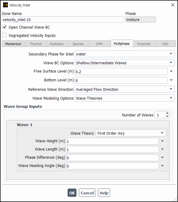
Secondary Phase for Inlet specifies the phase to which the wave parameters are applied. In case of a three-phase flow, select the corresponding secondary phase from this list.
Wave BC Options of which you have a choice of Shallow/Intermediate Waves, Short Gravity Waves, Shallow Waves, and None (for calm sea or pure open channel flow problems without waves). Information about these waves is available in Open Channel Wave Boundary Conditions in the Theory Guide. Note that the short gravity waves expression is derived under the assumption of infinite liquid height.
Free Surface Level is the same definition as for open channel flow, see Modeling Open Channel Flows.
Bottom Level is the same definition as for open channel flow, see Modeling Open Channel Flows, and is valid only for shallow or intermediate depth waves. The bottom level is used for calculating the liquid height.
Reference Wave Direction is the direction of wave propagation with zero wave heading angle. You can specify the wave propagation direction as:
Averaged Flow Direction: In this case, the reference direction is the same as the averaged flow direction.
Direction Vector
Normal to Boundary
Wave Modeling Options determines how the waves are modeled in the shallow/intermediate and short gravity wave regimes. You can choose to model the waves using either Wave Theories or Wave Spectrum. Wave Theories is usually selected for simulating regular waves. To simulate random waves, select Wave Spectrum.
Depending on your choice of Wave BC Options and Wave Modeling Options, you will need to specify the wave parameters as described in the following sections.
Shallow Wave Inputs
If you have selected Shallow Waves for Wave BC Options you can specify the following settings for each wave:
- Number of Waves
is the option to set the number of interacting waves (default = 1)
Ideally, shallow waves do not support the principle of superposition. The Number of Waves option enables interaction of two different waves originating at unique (non-interfering) locations within the domain. Collision of two counter-propagating solitary waves inside a domain is an example of a shallow wave interaction.
- Wave Theory
of which you have a choice of Fifth Order Solitary (the default) and Fifth Order Cnoidal. Information about the types of wave theory is available in Open Channel Wave Boundary Conditions in the Theory Guide.
- Wave Height
is the height difference between a wave crest to the neighboring trough.
Since a solitary wave does not have troughs, the wave height is the distance between a wave crest to mean free surface level.
- Wave Length
is the distance between two consecutive zero crossings.
Since solitary waves are derived based on the assumption of infinite wave length, specified wave length is only used to estimate the elliptic function parameter for suitability of the wave theory, and is not used in calculating wave parameters.
- Inlet Offset Distance
is the translational distance from the reference point origin in the reference wave propagation direction. This option is used to generate a wave from a location other than the reference frame origin. For a solitary wave, the hump is always generated at the location where:

(26–14)
where
 and
and  are spatial coordinates in the reference wave propagation
direction.
are spatial coordinates in the reference wave propagation
direction.- Wave Heading Angle
is the angle between the direction of the wavefront and the reference wave propagation direction, in the plane of the flow surface. In 2D, there are only two possibilities, zero degree when the wave is in the reference propagation direction, and 180 degree when the wave Is in the direction opposite to the reference propagation direction.
Wave Group Inputs
If you have selected Wave Theories for Wave Modeling Options you can specify the following settings for each wave:
- Number of Waves
is the option to set the number of superposed waves (default = 1)
- Wave Theory
of which you have a choice of First Order Airy (the default), Second Order Stokes, Third Order Stokes, Fourth Order Stokes, and Fifth Order Stokes. Information about the types of wave theory is available in Open Channel Wave Boundary Conditions in the Theory Guide.
- Wave Height
is the height difference between a wave crest to the neighboring trough.
- Wave Length
is the distance between two consecutive crests, troughs or zero crossings.
- Phase Difference
is the phase angle by which one periodic disturbance or wavefront lags behind or precedes another in time or space.
- Wave Heading Angle
is the angle between the direction of the wavefront and the reference wave propagation direction, in the plane of the flow surface. In 2D, there are only two possibilities, zero degree when the wave is in the reference propagation direction, and 180 degree when the wave Is in the direction opposite to the reference propagation direction.
Wave Spectrum Inputs
If you have selected Wave Spectrum for Wave Modeling Options you can specify the following settings for each wave:
- Frequency Spectrum Method
specifies the spectrum to use. You can select Pierson-Moskowitz (appropriate for fully-developed seas), Jonswap (appropriate for fetch-limited seas), or TMA (appropriate for fetch-limited, finite-depth seas).
- Peak Shape Parameter
controls the shape and amplitude of the frequency peak in the Jonswap and TMA formulations. This corresponds to
 in Equation 14–101 in the Fluent Theory Guide.
- Significant Wave Height
is the mean wave height of the largest 1/3 of waves. This corresponds to
 in Equation 14–100 in the Fluent Theory Guide.
- Peak Wave Frequency
is the wave frequency corresponding to the highest wave energy. This corresponds to
 in Equation 14–100 and Equation 14–101 in the Fluent Theory Guide.
  can be expressed in terms of the peak wave period,
  , as
, as  .
.- Minimum/Maximum Wave Frequency
specify the frequency range for the spectrum. Note that the Peak Wave Frequency must fall in between Minimum Wave Frequency and .
- Number of Frequency Components
specifies the number of components into which the frequency spectrum is divided.
specifies the method to use for specifying the directional spreading characteristics. You can choose Unidirectional (for long-crested waves), Frequency Independent Cosine Function (for short-crested waves where the directional component does not depend on frequency), and Frequency Dependant Hyperbolic Function (for short-crested waves where the directional component depends on frequency).
- Frequency Independent Cosine Exponent
specifies the exponent in the Frequency Independent Cosine Function formulation. This corresponds to
 in Equation 14–105 in the Fluent Theory Guide.
- Mean Wave Heading Angle
specifies the principal wave heading direction.
- Angular Spread
specifies the deviation from the mean wave direction for calculating the angular range.
- Number of Angular Components
specifies the number of components into which the angular range is divided.
The total number of wave components is the product of Number of Frequency Components and Number of Angular Components. For modeling random waves, phase differences for the individual wave components are randomly distributed between 0 and 2π.
Note: Any change in the input for Number of Wave Components will change the values of phase difference for each component. Therefore, it is recommended that you start the simulation from a saved case file after setting all the wave spectrum user inputs and that you not change the number of wave components during the simulation.
A useful text command used to print out a summary of the open
channel wave boundary condition settings is define/boundary-conditions/open-channel-wave-settings. The output will depend on whether you have chosen Wave
Theories or Wave Spectrum.
Sample Output for Wave Theories
/define/boundary-conditions> open-channel-wave-settings

Wave Input Analysis for Velocity Inlet : Thread ID = 5
************************************************************

Wave-1 Analysis
*****************************************

Current Settings :
------------------
Wave theory : 5th-order-Stokes , Wave regime = Shallow/Intermediate
Wave Height (H) = 0.2160, Wave Length (L) = 1.9400
Liquid Depth (h) = 0.6000, Ursell Number (H*L*L/(h*h*h)) = 3.7636

Mandatory checks for full wave regime within wave breaking limit
-----------------------------------------------------------------
Relative Height: H/h = 0.3600 , Maximum theoretical limit = 0.7800
Maximum numerical limit = 0.5500
Relative height within wave breaking limit

Wave Steepness: H/L = 0.1113 , Maximum theoretical limit = 0.1420
Stable numerical limit = 0.1000 , Maximum numerical limit = 0.1200
Warning: Wave steepness exceeding the stable numerical limit.
Waves could be stable or unstable in this regime.

Checks for selected wave theory within wave breaking and stability limit
----------------------------------------------------------------------------
Relative height check
H/h = 0.3600 , Min : 0.0000 , Max : 0.5000
Relative height check : successful

Wave Steepness check
H/L = 0.1113 , Min : 0.0000 , Max : 0.1363
Wave steepness check : successful

Ursell Number check
Ur = 3.7636 , Min : 0.0000 , Max : 25.0000
Ursell number check : successful

Wave regime check
h/L = 0.3093 , Min : 0.0600 , Max : 10000.0000
Wave regime check : successful

Summary
----------------------
Checks : passed
Selected wave theory is appropriate for application.
Sample Output for Wave Spectrum
Wave Input Analysis for Velocity Inlet : Thread ID = 6
************************************************************

Wave Spectrum Analysis
*****************************************

Current Settings :
------------------
Frequency Spectrum : Jonswap
Direction Spreading Method : Unidirectional

Significant Wave Height (Hs) = 5.0000
Peak Wave Frequency (wp) = 1.0000, Peak Time Period (Tp) = 6.2832
Minimum Frequency (wi) = 0.6600, Maximum Frequency (we) = 1.6600

Wave Lengths at Min/Peak/Max frequencies (Li, Lp, Le) = (141.5015, 61.6380, 22.3683)

Recommendation: Set the min and max wave frequencies so that most of the wave energy
  is concentrated in the selected regime of spectrum.
  - Min frequency = 0.5*Peak frequency
  - Max frequency = 2.5*Peak frequency


Wave Regime Check
----------------------
Wave regime type = Short Gravity (Deep)
Information: Validity of short gravity assumption : Liquid Depth > 0.5*Max Wave Length

Sea Steepness Check
-----------------------
Peak Time Period (Tp) = 6.2832
Zero Upcrossing Time Period (Tz) = 4.7869

Sea Steepness based on Tp (Sp) = 0.0811, Steepness Limit = 0.0667
Sea Steepness based on Tz (Sz) = 0.1398, Steepness Limit = 0.1000

Warning: Sea Steepness based on peak time period exceeding limit.
Warning: Sea Steepness based on zero upcrossing time period exceeding limit.

Information: High wave steepness of any individual component too could affect the wave pattern,
  as superposition of wave components is based upon lienar wave theory.

Frequency Spectrum Check
---------------------------
Peak Time Period to Wave Ht Sqrt Ratio (r = Tp/sqrt(Hs)) = 2.8099

Message: Selection of Jonswap spectrum is appropriate.

Recommended value of Peak Shape Parameter for r <= 3.6 :  5.0000

Spectrum Resolution check
----------------------------
Number of frequency components = 50
Number of angular components = 1
Total number of wave components = 50

Information: Higher number of wave components would have adverse effect on speed-up
  whereas smaller could affect the accuracy by not resolving the spectrum well.
  Following steps could assist to optimize the number of components
  1. Set number of frequency/angular components in boundary condition panel,
  2. Set TUI command solve> set> open-channel-wave-verbosity to 2 before initialization,
  3. Initialize (It would print Spectrum Energy for each frequency/angle.)
  4. Copy the information to plot Sw vs Omega and S_theta vs theta
  5. Optimize the number of components after repeating steps 1-4
Ansys Fluent supports transient profiles for all wave inputs using user-defined functions as seen by the example below:
/***********************************************************************
  UDF for defining transient profile wave inputs
 ************************************************************************/

#include "udf..h"

#define H 0.02 /* wave height for both waves : same */
#define LEN1 3. /* wave length for first wave */
#define LEN2 6. /* wave length for second wave*/
#define G 9.81
#define D 10. /* liquid depth */
#define U 1. /* wave current */
#define X 0. /* inlet point */

DEFINE_TRANSIENT_PROFILE(wave_ht, current_time)
{
	real k1 = 2.*M_PI/LEN1;
	real k2 = 2.*M_PI/LEN2;
	real w1 = sqrt(G*k1*tanh(k1*D)) + k1*U;
	real w2 = sqrt(G*k2*tanh(k2*D)) + k2*U;
	real dk = 0.5*(k1 - k2);
	real dw = 0.5*(w1 - w2);
	return (2.*H*cos(dk*X - dw*current_time));
}Fluent uses Fenton’s formulation for Stokes theories by default. For additional information about the current Stokes theories formulation, see Stokes Wave Theories in the Fluent Theory Guide. To revert to the old formulation, provided by Skjebreia and Hendrickson, use the following text command:
/solve/set/open-channel-wave-options> set-buffer-layer-ht set-verbosity stokes-wave-variants /solve/set/open-channel-wave-options>stokes-wave-variantsUse Fenton's formulation for Stokes wave theories [yes]noActivating old formulation (Skjelbreia and Hendrickson) for Stokes wave theories.
For additional information on the old formulation, refer to Lin’s book [89].
Once you have selected either the Open Channel Flow or the Open Channel Wave BC option in the Multiphase Model dialog box (Models tab), then the Open Channel Initialization Method drop-down list appears in the Solution Initialization task page.
![]() Solution →
Solution → ![]() Initialization
Initialization
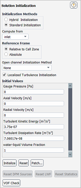
Select an inlet zone from the Compute from drop-down list. You can now make your selection from the Open Channel Initialization Method drop-down list. If only the Open Channel Flow option was enabled, then you only have a choice of None or Flat. If you enabled Open Channel Wave BC, then your choices are None, Flat, or Wavy. The default initialization method is None.
If you initialize the solution using None, it has no effect as it does not use any open channel information from the selected zone. The Open Channel Initialization Method comes into effect when you select either Flat or Wavy.
Important: This initialization is only valid for pressure-inlets, pressure outlets, and mass-flow inlets for open channel flow and velocity inlets for open channel wave boundary conditions. If the selected inlet zone does not have either open channel flow or open channel wave boundary conditions, Ansys Fluent will report an error message after you initialize the flow with open channel initialization method of Flat or Wavy.
For open channel initialization from the pressure outlet boundary, the hydrostatic pressure profile based on the Free Surface Level is patched in the domain. The volume fraction in the domain is patched based on Free Surface Level provided at the pressure outlet boundary. To patch velocity and other variables, the values in the Solution Initialization task page will be used.
Important: The pressure specification methods, with the exception of Free Surface Level, are not supported for open channel initialization from the pressure outlet boundary.
Initialization will result in the volume fraction, X, Y, and Z velocities, and pressure being patched in the domain. The volume fraction will be patched in the domain based on the free surface level of the selected zone from the Compute from list. The velocities in the domain will be patched assuming the constant value provided for the velocity magnitude in the selected zone.
Important: If you specify a profile for the velocity magnitude or direction vectors, the initialization will select the value for the velocity magnitude and direction vectors from only one face. Therefore the initialization may be inaccurate. However, generally, open channel inputs for velocity magnitude and direction vectors are constant.
The pressure that is patched is the hydrostatic pressure based on the free surface level specified in the selected zone.
You can use the following text command for open channel automatic initialization:
solve → initialize → open-channel-auto-init
When prompted, set up the following parameters:
- boundary thread id
Enter the thread id for the boundary to be selected for open channel automatic initialization.
- flat free surface initialization
This option is available for both open channel flow and open channel wave boundary conditions.
- wavy free surface initialization
This option appears only for open channel wave boundary conditions, when flat free surface initialization is not selected.
The steps to be followed for open channel automatic initialization are
Compute defaults based on valid open channel boundary thread. This step is required for better initialization of turbulence parameters based on uniform velocity magnitude.
solve→initialize→compute defaultsThis would provide information about the selected boundary and type of initialization.
solve→initialize→open-channel-auto-initInitialize
solve→initialize→initialize
To report values as wave speed, wave frequency, and time period for individual waves during initialization, you can set the following text command:
solve → set → open-channel-wave-options → set-verbosity
When prompted to set Verbosity for reporting of derived
wave inputs during initialization, enter 1 as shown below:
Note: You can enter values of 0, 1, or 2. Entering a higher number provides more information.
/solve/set/open-channel-wave-options>set-verbosityVerbosity for reporting of derived wave inputs during initialization [0]1
A sample of the resulting output for wave groups after initializing is shown below:
Wave-1 : Wave Height = 0.0200, Wave Length = 3.0000
Wave Number = 2.0944, Wave Speed = 2.1642, Wave Frequency = 4.5328
Effective parameters: Wave Speed = 3.1642, Wave Frequency = 6.6272, Time Period = 0.9481

Wave-2 : Wave Height = 0.0200, Wave Length = 6.0000
Wave Number = 1.0472, Wave Speed = 3.0607, Wave Frequency = 3.2052
Effective parameters: Wave Speed = 4.0607, Wave Frequency = 4.2524, Time Period = 1.4776

Time Period based on average effective frequency: 1.1550
The resultant output for Shallow Waves option is shown below:
Wave-1 : Wave Height = 0.2400, Specified Wave Length = 16.0000
Wave Number = 0.5051, Estimated Wave Length = 12.4398
Elliptic Function Parameter (m) : Calculated = 0.9976, Used = 1.0000
Liquid Height = 0.8000, Trough Height = 0.800000
Wave Speed = 3.1868, Wave Frequency = 1.6096
Effective parameters: Wave Speed = 4.1868, Wave Frequency = 2.1147
Time Period based on effective frequency: 2.9712
In certain applications, it is desirable to suppress numerical reflection near the outlet boundary for wave dampening. To understand the theory involved in this application, refer to Numerical Beach Treatment.
To include numerical beach in your simulation, perform the following:
Enable Gravity and set the gravitational acceleration fields.
Setup → General Gravity → On
Enable the Volume of Fluid model in the Multiphase Model dialog box (Models tab).
Setup → Models →
Multiphase → Edit...
In the Formulation group box, select either Implicit or Explicit.
Select Open Channel Flow and/or Open Channel Wave BC.
In order to set the numerical beach parameters for a fluid zone, go to the Fluid dialog box (Figure 26.34: The Fluid Dialog Box to Enable Numerical Beach).
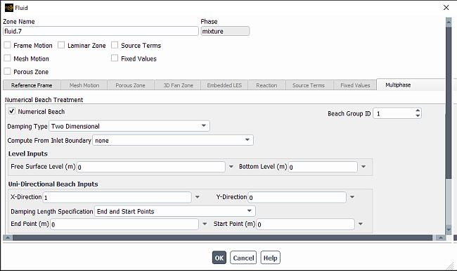
In the Multiphase tab of the Fluid dialog box, enable the Numerical Beach option and enter the following:
Beach Group ID represents the cell zones sharing the damping length containing the same input parameters.
Multi-Directional Beach helps to suppress the numerical reflections that arise from multiple open-channel pressure outlet boundaries. This is desirable while modeling oblique waves or when the pressure-outlet boundaries are closer to the zone of interest. (Only available for 3D problems.)
Uni-Directional Beach: should be used to suppress the numerical reflections from a single open channel pressure outlet. This is the case when the flow is generally uni-directional.
Damping Type allows you to choose between Two Dimensional and One Dimensional.
Two Dimensional is the damping treatment in the beach and gravity direction.
One dimensional is the damping treatment in the beach direction.
Compute From Inlet Boundary is set to none by default. If there are available open channel boundaries (velocity-inlet, pressure-inlet, and mass-flow-inlet), boundary names are added to the drop-down list. If you select a boundary from the list, the Level Inputs, Uni-Directional Beach Inputs or Multi-Directional Beach Inputs in beach direction, and Damping Resistance values will be updated in the interface. You have the option to overwrite the updated inputs with values that are more applicable to your simulation.
Level Inputs is only available for the Two Dimensional damping type.
Free Surface Level is the same definition as for open channel flow, see Modeling Open Channel Flows.
Bottom Level is the same definition as for open channel flow, see Modeling Open Channel Flows. During the automatic calculation from the velocity inlet boundary for short gravity waves, this parameter is updated under some assumptions, as noted in Solution Strategies. The bottom level is used for calculating the liquid height.
Numerical Beach Inputs
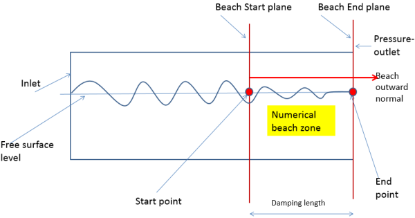
Numerical beach is assumed as a rectangular domain, where its end-plane (outer surface) is an open channel pressure outlet boundary and start-plane is a plane parallel to a pressure outlet. Beach direction is assumed as the direction normal to a pressure outlet. Damping length is the normal distance between the end and start plane.
- Uni-Directional Beach Inputs:
X, Y, and Z are the vector components of the beach outward normal (typically normal to the nearest pressure outlet).
The end point is calculated by taking the dot product of beach direction with any point lying on the end plane. Similarly, the start point is calculated as the dot product of beach direction with any point lying on the start-plane.
Note: The automatically calculated value of the end point is assumed based on the domain extents for all of the cell zones. Enter your own value if required.
Damping Length Specification is only available if Open Channel Wave BC is enabled in the Multiphase Model dialog box (Models tab). There are two options you can choose from:
End Point and Wave Lengths (default).
End and Start Points are the limits of the damping zone.
- Multi-Directional Beach Inputs
Number of Beach
The default is 2, the maximum is 3.
X-Direction
Y-Direction
Z-Direction
End Point
Damping Length
See Figure 26.35: Numerical Beach Sketch for a visual representation of the numerical beach.
Relative Velocity Resistance Formulation calculates the source term using relative velocities in the numerical beach zone when using moving/deforming meshes or moving reference frames.
Linear Damping Resistance is the resistance per unit time.
Quadratic Damping Resistance is the resistance per unit length.
Below are some helpful key points when using the Numerical Beach option:
The Compute from Inlet Boundary drop-down list is a convenient feature as it provides automatic inputs, which you should check to make sure the values are reasonable. Some of the provided values are calculated under certain assumptions:
The bottom level, in the case of short gravity waves, is selected in the velocity inlet dialog box for open channel wave boundary conditions. Since there is no user input for this parameter, Ansys Fluent calculates the bottom level as the value of the free surface level less 2.5 times the wave length. The assumption is that the liquid height is 2.5 times the wave length.
The automatically calculated value of the end point is assumed based on the domain extents for all of the cell zones.
For manual inputs of start and end points, you should verify that these points are calculated correctly in the beach direction. To check for their validity, subtracting the start point from the end point should give you a positive value.
For manual inputs of Free Surface Level and Bottom Level, you should verify that these points are calculated correctly in the direction opposite to gravity. To check for their validity, subtracting the bottom level from the free surface level should give you a positive value.
In case you create separate damping zones, but the damping length is not sufficient to suppress the waves, clubbing of the beach could be done by selecting the same beach ID for other cell zones. In this case, both the cell zones would share the same information.
In case of separate damping zones (without clubbing), you should verify that the damping length is more than or equal to the specified number of wave lengths for the calculation of the start point.
Damping resistance should be chosen carefully as too much or too little damping could affect the wave profiles in a no-damping zone. The Compute From Inlet Boundary option automatically populates the values for damping resistances based on analytical correlations for wave energy. However, you may need to further tune these values for certain cases if the computed values are found to be unsuitable.
Steep damping at the beginning of the damping zone could affect the wave profile just before the damping zone.
It is recommended that you use a coarse mesh in the damping zone with increased coarseness towards the end of the damping zone.
Instructions for specifying the necessary information for the primary and secondary phases and their interaction in a VOF calculation are provided below.
Important: In general, you can specify the primary and secondary phases whichever way you prefer. It is a good idea, especially in more complicated problems, to consider how your choice will affect the ease of problem setup. For example, if you are planning to patch an initial volume fraction of 1 for one phase in a portion of the domain, it may be more convenient to make that phase a secondary phase. Also, if one of the phases is a compressible ideal gas, it is recommended that you specify it as the primary phase to improve solution stability.
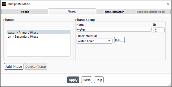
To define the primary phase in a VOF calculation, perform the following steps:
In the Multiphase Model dialog box, go to the Phases tab.
Setup
→ Models → Multiphase
Edit...
From the Phases list, select the phase (for example, phase-1).
In the Phase Setup group box, enter a Name for the primary phase (for example,
water).Specify which material the phase contains by choosing the appropriate material in the Phase Material drop-down list.
Define the material properties for the selected phase material.
Click next to Phase Material.
In the Edit Material dialog box, check the properties, and modify them if necessary. (See Physical Properties for general information about setting material properties, Modeling Compressible Flows for specific information related to compressible VOF calculations, and Modeling Solidification/Melting for specific information related to melting/solidification VOF calculations.)
Important: If you make changes to the properties, remember to click before closing the Edit Material dialog box.
Click .
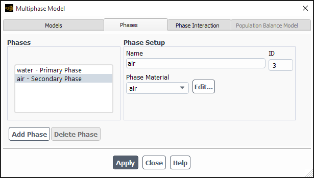
The procedure for defining a secondary phase in a VOF calculation is similar to that for the primary phase:
Select the phase (for example, phase-2) from the Phases list.
In the Phase Setup group box, enter a Name for the phase (for example,
air).Specify which material the phase contains by choosing the appropriate material in the Phase Material drop-down list.
Define the material properties for the Phase Material, following the procedure outlined above for setting the material properties for the primary phase.
Click .
As discussed in When Surface Tension Effects Are Important in the Theory Guide, the importance of surface
tension effects depends on the value of the capillary number, Ca (defined by Equation 14–32 in the Theory Guide), or the Weber number, We
(defined by Equation 14–33 in the Theory Guide). Surface tension effects can
be neglected if Ca  or We
or We  .
.
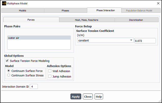
You can include the effects of surface tension along the interface between one or more pairs of phases, as described in Surface Tension and Adhesion in the Theory Guide, in the Phase Interaction > Forces tab of the Multiphase Model dialog box (Figure 26.38: The Multiphase Model Dialog Box (Forces Tab)).
![]() Setup → Models
→ Multiphase
Setup → Models
→ Multiphase
![]() Edit...
Edit...
Perform the following steps to model surface tension (and, if appropriate, include adhesion) effects along the interface between one or more pairs of phases:
In the Global Options tab, enable the Surface Tension Force Modeling option to include the surface tension method. You can specify the Surface Tension Coefficients as constant, polynomial, piecewise-linear, piecewise-polynomial, or user-defined. You can also use RGP tables to specify Surface Tension Coefficients as described in Defining Saturation Properties via RGP Tables.
Note: If none is selected, then Surface Tension Force Modeling will automatically be disabled.
Select the surface tension method that is most applicable to your case. You can choose between Continuum Surface Force and Continuum Surface Stress. Information about each of the methods is described in Surface Tension in the Theory Guide.
For each pair of phases between which you want to include the effects of surface tension, specify an input for the surface tension coefficients using one of the following options:
Constant Value
Temperature-dependent polynomial, piecewise polynomial, or piecewise linear
These options are available only while modeling energy.
User-defined surface tension coefficient
This can be defined as a function of any space variable or time.
See Surface Tension and Adhesion in the Theory Guide for more information on surface tension, and the Fluent Customization Manual for more information on user-defined functions. All surface tension coefficients are equal to 0 by default, representing no surface tension effects along the interface between the two phases.
Important: For calculations involving surface tension, it is recommended that you also turn on the Implicit Body Force treatment for the Body Force Formulation in the Multiphase Model dialog box (Models tab). This treatment improves solution convergence by accounting for the partial equilibrium of the pressure gradient and surface tension forces in the momentum equations. See Including Body Forces for details.
If you want to include wall adhesion, enable the Wall Adhesion option and then specify the contact angle at each wall as a boundary condition (as described in Steps for Setting Boundary Conditions).
If you want to include jump adhesion, enable the Jump Adhesion option. When Jump Adhesion is enabled, you will need to specify the contact angle at the porous jump in the Porous Jump dialog box (as described in Defining Multiphase Cell Zone and Boundary Conditions). The contact angle specification and measurement for jump adhesion is similar to that of wall adhesion (as explained in step 3 above).
Important: Jump adhesion only supports the cell based smoothing option for surface tension. When the Jump Adhesion option is enabled in the Global Options group box, the correct settings are automatically set for surface tension. To view the surface tension settings, use the
solve/set/surface-tensiontext command.Click Apply.
Note: The following limitations exist:
When the Wall Adhesion and Jump Adhesion options are enabled, you must specify a nonzero surface tension coefficient.
Jump Adhesion is not available with the Continuum Surface Stress model.
The Continuum Surface Stress model and the Jump Adhesion option are not available with the Coupled Level Set + VOF option.
Several surface tension options are provided through the text user interface (TUI)
using the solve/set/surface-tension command :
solve → set →
surface-tension
The surface-tension command prompts you for the following
information:
whether you require node-based smoothing
The default value is
yes, indicating that node-based smoothing will be used. Note that if you are reading in a case that was created in versions prior to Ansys Fluent 13, then cell-based smoothing will be used by default.the number of smoothings
The default value is
2, which is suitable for most cases. A higher value can help in reducing spurious currents for highly skewed and non-uniform meshes. Note that for cases created in versions prior to Ansys Fluent version 2020 R1, only single smoothing will be used by default.the smoothing relaxation factor
The default is
1. This is useful in the cases where volume fraction smoothing causes a problem (for example, liquid enters through the inlet with wall adhesion on).whether you want to use volume fraction gradients at the nodes for curvature calculations
With this option, Ansys Fluent uses volume fraction gradients directly from the nodes to calculate the curvature for surface tension forces. The default is
yeswhich produces better results with surface tension compared to gradients that are calculated at the cell centers.
When Surface Tension Force Modeling is enabled, the following additional variables become available for postprocessing under the Phases... category:
Smoothed VOF Gradient-dX, Smoothed VOF Gradient-dY, and Smoothed VOF Gradient-dZ
Smooth VOF Gradient Magnitude
See Field Function Definitions for their definitions.
Important:
Note that the calculation of surface tension effects will be more accurate if you use a quadrilateral or hexahedral mesh in the area(s) of the computational domain where surface tension is significant. If you cannot use a quadrilateral or hexahedral mesh for the entire domain, then you should use a hybrid mesh, with quadrilaterals or hexahedra in the affected areas.
Ansys Fluent uses node based smoothing for smoothed volume fraction and node based gradients for smoothed curvature calculation to provide better accuracy and robustness.
Pressure jump caused by the surface tension is discontinuous in nature, and also it acts locally at the interface. These numerical difficulties are overcome in an approximate manner by considering the smoothed distribution of the volume fraction field within the finite interfacial width. Smoothing procedures, in general, are mesh dependent. Therefore, the amount and nature of the smoothing procedure could have a significant effect on the results for surface tension cases.
Most of the interface capturing or tracking schemes, which are common in literature, can simulate either diffused interface modeling or sharp interface modeling. There are a number of applications where you may be interested in modeling diffused and sharp interfaces in different regimes, which results in the need for a unique discretization procedure to handle such applications.
Below are some examples of such applications:
Air bubble rise in water-solid slurry: Diffused interface modeling is required for the water and solid, and sharp interface modeling for the air bubble is desirable. A sharpening scheme would cause undesirable effects for the modeling of the diffused interface between water and solids and a diffusive scheme would not be able to maintain the sharp interface for bubble rising in the slurry.
Evaporation/condensation in a tank partially filled with water and being heated at the bottom: Diffused interface modeling is required for the liquid-vapor and sharp interface modeling for the water-air regime is desirable. A sharpening scheme, would not be able to simulate the diffused phenomena of evaporation/condensation for the liquid- vapor phase and a diffusive scheme would not be able to maintain the sharp interface between water and air.
Air jet penetrating through layer of liquids: You may be interested in diffused jet modeling and sharp interface modeling between the liquid layers. A sharpening scheme would not be able to maintain the continuous air stream and a diffusive scheme would not be able to maintain the sharp interfaces between the layers of liquids.
Using the Modified HRIC and Compressive schemes for such applications would result in the HRIC scheme producing undesirable sharpening of the dispersed phases and undesirable diffusion of the continuous phases, whereas the Compressive scheme would produce undesirable sharpening of the dispersed phases.
Therefore, the phase localized compressive scheme is particularly useful in cases where the desirable behavior is such that you have diffused modeling of dispersed phases and sharp modeling of continuous phases. In Ansys Fluent, diffusive and anti-diffusive discretization procedures can be used across the distinct interfaces, which share a pair of phases. This functionality is provided through the compressive discretization scheme, where the degree of diffusion or sharpness is controlled through the value of the slope limiters. The theory used is described in The Compressive Scheme and Interface-Model-based Variants.
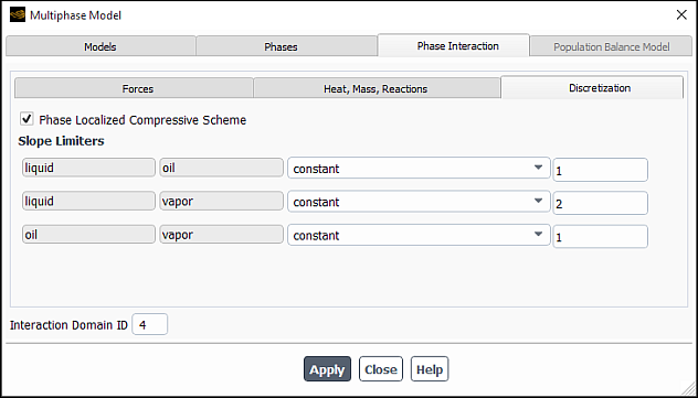
To use the phase localized compressive scheme, perform the following steps:
Click the Discretization tab.
Note: The Discretization tab is available for the VOF model, Mixture multiphase model, and Eulerian multiphase model with Mulit-Fluid VOF only when the Phase Localized Discretization option is enabled in the Interface Modeling Options dialog box. (Interface Modeling Type).
Enable Phase Localized Compressive Scheme.
Important: When this option is enabled, the Compressive spatial discretization scheme is automatically selected for the Volume Fraction in the Solution Methods dialog box.
For each pair of phases, specify the value of the slope limiter. You can enter a value of 0, 1, or 2, or any value between 0 and 2. Refer to Table 26.11: Slope Limiter Discretization Scheme to equate each value of the slope limiter with a discretization scheme.
Table 26.11: Slope Limiter Discretization Scheme
Slope Limiter Value 
Scheme 0 first order upwind 1 second order reconstruction bounded by the global minimum/maximum of the volume fraction 2 compressive  and
and 
blended: where a value between 0 and 1 means blending of the first order and second order and a value between 1 and 2 means blending of the second order and compressive scheme
When using the Phase Localized Compressive Scheme, note the following:
The minimum limit for the slope limiter is 0, whereas the maximum is 2.
The slope limiter can be interpreted as the degree of compression/anti-diffusion, where 0 demonstrates the minimum compression and 2 demonstrates the maximum compression.
For interfaces sharing the diffused phases, a slope limiter value of 2 should not be used. A value between 0 and 1 is recommended.
For interfaces sharing the continuous phases, any value between 0 and 2 can be used depending on the application.
For interfaces sharing the continuous and diffused phases, any value between 0 and 2 can be used based on the application.
If you want variable discretization behavior for an interface between two phases, you can do so via the
DEFINE_PROPERTYuser-defined function.
Note:If the interface has a transition from sharp to diffused modeling, you should not experience any problems.
If the interface has a transition from diffused to sharp modeling, this transition should be smooth by gradually varying the value of the slope limiter within some transition zone.
If you are using the Explicit volume fraction formulation in Ansys Fluent, an explicit solution for the volume fraction is obtained either once each time step or once each iteration, depending upon your inputs to the model. You also have control over the time step size used for the volume fraction calculation.
You can access the controls for the volume fraction in the Expert Options dialog box that opens by clicking Expert Options... in the Multiphase Model Dialog Box (Models tab).
For the time-dependent calculation for the VOF model, you need to specify the following settings:
- Sub-Time Step Calculation Method
When Ansys Fluent uses the Explicit formulation, the time step size used for the volume fraction calculation will not be the same as the time step size used for the rest of the transport equations. Ansys Fluent will refine the time step size for VOF automatically, based on your input for the maximum Courant Number allowed near the free surface. The Courant number is a dimensionless number that compares the time step size in a calculation to the characteristic time of transit of a fluid element across a control volume.
The characteristic transit time for a fluid element across the control volume represents the time taken by the fluid to empty out of the cell. This transit time is taken as the smallest of such time in the region near the fluid interface. A sub time step size, for use in the VOF calculations, is computed based on this characteristic time, and the maximum allowed Courant Number set in the Multiphase Model Dialog Box (Models tab). For example, if the maximum allowable Courant Number is
0.25(default), the computed sub time step size will have a maximum value equal to a quarter of the minimum transit time for any cell near the interface.In Fluent, the sub time step size for VOF calculations can be computed using the following options:
Velocity Based: The sub time step size is estimated by the cell size and the fluid velocity normal to the interface:

(26–15)
where,
 is the Courant Number,
  is the relative velocity of the fluid, and
  is the cell size.
Flux Based: For this option, the sub time step size is estimated based on the cell volume and the summation of outgoing fluxes in the cell:

(26–16)
where,
 is the Courant Number,
  is the volume, and
  are the outgoing fluxes.
Flux Averaged: The sub time step size is estimated by volumetric averaging the calculations of the Flux Based method for the neighboring cells.
Hybrid: This is the default method for calculating sub time step size. The sub time step size is estimated by blending the Velocity Based and Flux Averaged calculation methods.
Note:The Flux Based calculation method is the most conservative sub-time step size estimation, while the Velocity Based calculation is the most aggressive. Flux Averaged and Hybrid methods fall in between for most cases.
Aggressive sub time step calculation methods generally save time during interface reconstruction. However, the aggressive method can lead to increased number of iterations due to larger transient errors being introduced while integrating over the sub time steps for the interface reconstruction.
During the simulation, the Global Courant Number [Explicit VOF Criteria] is printed in the console. It is calculated using the previously computed sub-time step
 as:
as:where
 is the maximum allowed Courant number, and
  is the global time step.
- Solve VOF Every Iteration
By default, Ansys Fluent will solve the volume fraction equation(s) once for each time step. This means that the convective flux coefficients appearing in the other transport equations will not be completely updated each iteration, since the volume fraction fields will not change from iteration to iteration.
When Ansys Fluent solves these equations every iteration, the convective flux coefficients in the other transport equations will be updated based on the updated volume fractions at each iteration. This choice is the less stable of the two, and requires more computational effort per time step than the default choice.
Important: If you are using sliding meshes, or dynamic meshes with layering and/or remeshing, using the Solve VOF Every Iteration option will yield more accurate results, although at a greater computational cost.

If you are including melting or solidification in your VOF calculation, note the following:
It is possible to model melting or solidification in a single phase or in multiple phases.
For phases that are not melting or solidifying, you must set the latent heat (
 ), liquidus temperature (
 ), and solidus temperature (
 ) to zero.
See Modeling Solidification and Melting for more information about melting and solidification.
For the analysis of dispersion of liquid in gas, two principal multiphase flow methodologies can be applied:
In the Euler-Lagrange approach, discrete droplets are tracked through the domain. The particle tracker uses physical properties of individual droplets in order to account for the exchange of mass, momentum, heat, species (and so on) with the continuous phase. The gas volume displacement by the droplets is ignored. This approach is relatively computationally inexpensive because it allows the mesh to be coarser than the size of a droplet. The secondary breakup can be modeled relatively accurately using known breakup models. However, in the dense region of a spray, simulation accuracy may suffer from neglecting the volume displacement. Also, in regions where the spray does not consist of discrete spherical droplets, special models must be used to predict the primary breakup of the initial contiguous liquid jet. These models must be derived from experimental data based upon the operating conditions for each injector.
In the volume-of-fluid (VOF) approach, the volume fraction of the liquid is stored in each cell. The gas-liquid interface can be tracked by explicit discretization schemes, such as geometric reconstruction. The VOF model requires a much higher mesh resolution and a much smaller time step size. The phase boundary around every droplet must be resolved by a mesh that is significantly finer than the finest droplets. This allows for better predictions of the primary breakup. The volume displacement is inherently accounted for, which can be important for the dense region of the dispersed spray. However, this method is expensive and requires large HPC resources.
Ansys Fluent provides the capability to combine the two approaches described above by using a VOF-to-DPM model transition mechanism. The initial jet and primary breakup are predicted using the VOF model on a sufficiently fine mesh, while the voluminous dilute region of the dispersed spray is simulated by the DPM. The VOF-to-DPM model transition algorithm automatically finds compact liquid masses that have detached from the liquid core in the VOF solution. It then assesses their eligibility for the VOF-to-DPM model transition. If the liquid lump satisfies user-specified criteria, such as lump size and asphericity (that is, relative or normalized deviation from the shape of a perfect sphere), it is removed from the resolved liquid in the VOF simulation and converted to a particle parcel in the Lagrangian formulation. Any local solution-adaptive mesh refinement used to resolve the gas-liquid interface is automatically reverted, so that the Lagrangian particle parcel can be placed in a single large cell. If the volume of a liquid lump is much larger than the volume of the coarsened mesh cell, then the lump will be converted into as many Lagrangian particle parcels as the number of cells spanned by the lump such that the volume of each parcel will be equal to its corresponding cell volume. In early stages after the conversion, the group of particle parcels representing the liquid droplet will travel together, but as they proceed through the domain, their paths may gradually diverge.
Converting liquid lumps to Lagrangian parcels does not impose volume displacement on the continuous-phase VOF flow simulation. In order to avoid spurious momentum sources, a volume of gas with the same volume as the liquid lump is created in the VOF simulation to maintain the volume conservation. The mass source that is equivalent to the mass of the gas volume will affect the overall mass balance.
This approach can be used for simulating liquid atomization in gas turbines, internal combustion engines, and other similar applications.
Such simulations usually require high spatial and temporal resolution to capture all the relevant details of a primary atomization process of a liquid jet. Resource limitations will restrict this approach to detailed analyses in regions near the nozzle. For the complete simulation of a spray system or process, it is recommended that all information about the Lagrangian DPM particle parcels be captured and transferred into a separate simulation that only uses the Euler/Lagrange approach because it allows a coarser mesh and larger time step size to be used.
This can be achieved, for example, by using DPM particle sampling on either a cut plane
or the outlet boundary of the domain of the detailed VOF-to-DPM simulation. For unsteady
particle tracking, the sampling feature writes information into a file for every particle
parcel that crosses the sampling plane or boundary. The file can then be used as an unsteady
injection file for another unsteady particle tracking simulation. Ansys Fluent will recreate
each particle parcel at the same location and instance in simulated time
(flow-time in the injection file).
An alternative to using DPM particle sampling for creating such a file is to use the VOF-to-DPM built-in functionality as described below. If you provide a filename, the solver will write a new file containing information for each liquid lump that has been converted. The file has the same format as a DPM sample file for unsteady particle tracking. Therefore, it can be read into a separate DPM simulation as an unsteady injection file.
The VOF-to-DPM model transition feature cannot be used with the following:
Steady-state flow
Multi-fluid VOF
Steady DPM particle tracking
The Level Set model
The identification of individual lumps and the calculation of the lump properties do not account for special boundary conditions such as symmetry and periodicity (including periodic non-conformal interfaces). A liquid lump that touches a symmetry boundary is treated as if it was attached to a wall. A lump that intersects a periodic boundary is treated as multiple independent lumps. In both cases, the values calculated for the lump properties, particularly the asphericity, will be affected.
Important: The VOF-to-DPM model transition mechanism is available only for 3D cases.
To use the VOF-to-DPM Model Transition capability, follow the steps below:
When generating the mesh for your analysis, avoid high-aspect-ratio cells. Adjust the mesh resolution so that four or five levels of adaption will be sufficient for resolving the finest structures when you are using the VOF calculation.
If appropriate, define the automatic solution-adaptive mesh refinement.
 Domain → Adapt
→ Automatic...
Domain → Adapt
→ Automatic...
For example, if you just want to make sure that the phase boundary is resolved with the highest possible mesh resolution, you can use cell registers that apply the Curvature method to the phase volume fraction in order to coarsen all cells with a value below 1.e-10 and refine all cells with a value above 1.e-08. Make sure to use a small Frequency (such as 1 or 2).
If the resolution of the initial mesh is not uniform, you can specify a minimum edge length in the General Adaption Controls dialog box in order to avoid excessively small cells (and therefore high CFL numbers), or when multiphase-specific time stepping is used, to avoid excessively small time-steps. If a sufficient number of refinement levels is specified, the adapted mesh at the liquid/gas interface will have little variation in cell volume, regardless of the local resolution in the initial mesh.
Note that an easy way to set up the adaption for VOF simulations is to use the Predefined Criteria drop-down list, as described in VOF Adaption. This list allows you to select from commonly used criteria for adapting the mesh; the Multiphase... submenu provides options for VOF, including VOF-to-DPM [Generic] (which uses fairly straightforward cell registers) and VOF-to-DPM [Advanced] (which uses more complex expressions).
If you use hanging nodes to create the initial mesh, make sure that you use the default polyhedral unstructured mesh adaption (PUMA) for the automatic solution-adaptive mesh refinement, because the hanging node adaption method will skip two cell layers on the coarse side of the hanging nodes. To select PUMA, use the following text command:
mesh/adapt/set/method2In the Discrete Phase Model dialog box, select Unsteady Particle Tracking.
Physics → Models
→ Discrete Phase...
Create a DPM injection of any type as usual and specify a very large value for Start Time. This will guarantee that no particles will be injected at the specified location.
Setup → Models
→ Discrete Phase
→ Injections New...
In the Models tab of the Multiphase Model dialog box, configure the following settings.
Physics → Models
→ Multiphase...
Tab
Setting
Value
Model
Volume of Fluid
(Selected)
Volume Fraction Parameters
Formulation
Explicit
Interface Modeling
Type
Sharp
Body Force Formulation
Implicit Body Force
(Selected)
In the Phase Interaction tab of the Multiphase Model dialog box, define the correct surface tension for the gas-liquid boundary.
In the Solution Methods task page, configure the following solution parameters.
Solution → Solution
→ Methods...
Group Box
Setting
Value
Pressure-Velocity Coupling
Scheme
PISO
Spatial Discretization
Volume Fraction
Geo-Reconstruct
Pressure
PRESTO!, Body Force Weighted, or Modified Body Force Weighted
If you selected PISO for the Pressure-Velocity Coupling scheme, increase the Pressure and Momentum Under-Relaxation Factors to values close to 1 (for example, 0.98) in the Solution Controls task page.
Solution → Controls
→ Controls...
In the Phase Interaction > Model Transition tab, define VOF-to-DPM model transition.
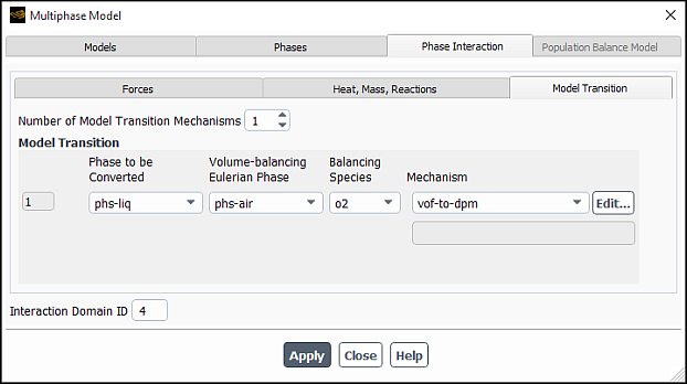
Specify the Number of Model Transition Mechanisms.
For each mechanism, select the liquid phase from the Phase to be Converted drop-down list and also the gas phase from the Volume-balancing Eulerian Phase drop-down lists.
Lagrangian particle parcels do not have any volume displacement effect on any VOF phase. Therefore, in order to maintain volume conservation in the VOF solution, when liquid from the VOF solution is converted into one or more Lagrangian particle parcel(s), an equal volume of the selected gas phase is placed into the VOF solution as a replacement for the converted liquid.
For each pair of phases with model transition, select vof-to-dpm from the Mechanism drop-down list.
In the VOF-to-DPM Transition Parameters dialog box that opens automatically, specify the parameters for the model transition:
- Frequency
specifies the frequency at which the VOF-to-DPM model transition mechanism is run. That is, this parameter denotes the number of time steps between consecutive VOF-to-DPM model transition passes for the individual model transition mechanism.
- Injection
is a list of available injections. Make sure you select the injection that you created earlier for the VOD-to-DPM model transition. All newly created particle parcels will be assigned to the selected injection.
- Coarsen the Mesh Immediately where Lumps are Transitioned
specifies whether the mesh should be coarsened when a liquid lump is converted to a DPM particle parcel and removed from the VOF solution. The coarsening is achieved by reverting all previously dynamically added mesh refinements. This option is selected by default and recommended.
- Split any DPM Parcel that Exceeds the Cell Volume by Factor
specifies a ratio used for determining the number of DPM parcels into which the liquid lump is divided. If the liquid lump volume does not exceed the volume of the coarsened cell multiplied by this factor, the lump is converted into one parcel containing one particle. Otherwise, the lump is split into as many parcels as there are cells covered by the original liquid lump. To conserve mass, the number of particles per parcel is reduced from unity such that the sum of all parcels resulting from the split represents exactly the mass of the original liquid lump.
The splitting of a single lump into multiple particle parcels may be needed if there is a risk that DPM source terms may cause instabilities in the continuous phase flow solution. This may happen for cases with evaporation or boiling and a fine background mesh.
As long as you do not encounter any stability issues in the continuous phase flow solution, you can set a very high value for this factor in order to prevent lumps from splitting into multiple parcels. However, if the factor is set relatively low, a lump may split into multiple parcels. These parcels are mutually independent and therefore may disperse. Splitting parcels does not change the global size distribution, but they may affect the spatial distribution of parcels of different sizes throughout the spray.
- VOF Lump Transition Requirements
contains parameters for specifying conversion eligibility limits.
- Volume-Equivalent Sphere Diameter Range
sets the Minimum and Maximum diameter values for a volume-equivalent sphere. Liquid droplets found in the VOF solution whose volume is outside this range will not be converted to Lagrangian particle parcels.
- Upper Limits of Asphericity as Calculated by
- Radius Standard Deviation
specifies the maximum asphericity calculated from the normalized radius standard deviation. This quantity is calculated for every liquid lump found in the VOF solution as follows. For every facet of the lump surface (gas-liquid phase interface), the distance between the facet center and the lump center of gravity is calculated. The individual distance values are weighted by the size of the individual lump boundary facet. Their standard deviation is computed and then normalized by the average radius.
This quantity is zero for perfect spheres and increasingly greater than zero the more the shape deviates from a sphere. All droplets for which the asphericity value is below the specified maximum may be automatically elected for conversion. The default value for Radius Standard Deviation is 0.5.
- Radius-Surface Orthogonality
specifies the maximum asphericity calculated from the average radius-surface orthogonality. This quantity is calculated for every liquid lump found in the VOF solution as follows. For every facet of the lump surface (gas-liquid phase interface), a vector from the lump's center of gravity to the center of the lump boundary facet is computed. This vector is normalized and then used in a dot product with the facet unit normal to yield a measure of a relative orthogonality ranging from 0 to 1. For a perfect sphere, the value would all be 1. A facet area-weighted average of these values is then subtracted from 1 to obtain the asphericity value.
For almost spherical droplets, this quantity is significantly closer to 0 than the standard deviation-based asphericity. For more drastically non-spherical lumps, it produces values comparable to those obtained with the standard deviation-based asphericity. The default value for Radius-Surface Orthogonality is 0.5.
- Lump Conversion Transcript
(optional) specifies a name for the file where Ansys Fluent will save the DPM particle variables corresponding to each VOF lump that is converted. The file contains one line for each converted lump, regardless of whether a lump was converted into one or multiple DPM parcels. The file is written in the same format that is used for particle sampling (see Sampling of Trajectories).
As with any sample file written by unsteady particle tracking, this file can be used as an unsteady injection file. This makes it possible to calculate the small dense region of a spray using the VOF-to-DPM model transition mechanism and the much larger dilute region in a pure DPM calculation that uses the lump conversion transcript as an injection file. For better control over the number of the numerical particle parcels, the injection file can be run through the file reduction tool as described in Data Reduction of Samples.
If you use a
DEFINE_DPM_OUTPUTUDF to write the particle sampling file, the same UDF will be used to write the lump conversion transcript file. The UDF gives you control over the file content and it even allows you to modify the DPM particle parcels generated from the liquid lumps during the VOF-to-DPM model transition. For details, seeDEFINE_DPM_OUTPUTin the Fluent Customization Manual.You can use the
DEFINE_DPM_OUTPUTUDF to add additional DPM variables to the output file in extra columns. If you then use that lump conversion transcript file as an unsteady injection file in a separate simulation, you can use aDEFINE_DPM_INJECTION_INITUDF to read the additional columns and use the data to initialize the additional DPM variables. For details, seeDEFINE_DPM_INJECTION_INITin the Fluent Customization Manual.- Use this Mechanism for Lump Postprocessing
when selected, Ansys Fluent uses the mechanism settings for the calculation of the postprocessing lump detection quantities. See Postprocessing for VOF-to-DPM Model Transition Calculations for information about postprocessing lump detection quantities.
- Consider Diffuse Lumps
when selected, distinct liquid lumps that for some numerical reason started to be smeared out in the mesh before they detached fully from the contiguous liquid jet will be converted to Lagrangian particle parcels. You can specify the following Diffuse Lump Transition Requirements in the Lump Core Highest Volume Fraction group box:
- Minimum
controls the conversion of distinct liquid lumps. If the highest VOF liquid volume fraction within the lump is below the specified value, the lump will not be converted. The default value is 0.9.
- Maximum
can be used to restrict the conversion to diffused lumps only. If the highest VOF liquid volume fraction within the lump is above the specified value, the lump will not be converted. The default value is 1.1. Note that although the volume fraction cannot exceed unity, the default value of 1.1 is used to prevent roundoff errors.
The VOF-to-DPM solver finds the highest VOF liquid volume fraction within each eligible lump that meets all other criteria. Only if this value lies within the specified range will the lump be converted to the DPM Lagrangian particle parcel.
Refer to Best Practice Guidelines for Considering Diffuse Lumps for tips for using the Consider Diffuse Lumps option.
The liquid lumps having dimensions within the specified lump diameter range and falling below both the asphericity criteria will be elected for conversion to DPM parcels.
In order to see typical asphericity values for the droplets in your simulation, you can, for example, create contour plots of the asphericity field functions on an iso-surface of a volume fraction of 0.5.
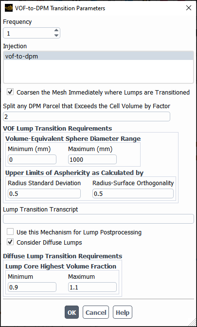
The Consider Diffuse Lumps option (see Setting up the VOF-to-DPM Model Transition) can be useful in the following scenario.
In industrial VOF-to-DPM calculations, some diffused VOF liquid structures may not be converted to Lagrangian parcels although they have obviously detached from the main liquid jet. If the automatic solution-adaptive mesh refinement has been set up such that it keeps every cell that contains any liquid (or is in close vicinity to such a cell) refined, then these liquid lumps can greatly increase computational time.
The following strategy helps to minimize the occurrence of such diffused liquid lumps.
In the Phase Interaction dialog box, under the Model Transition tab, define the following three vof-to-dpm mechanisms. The mechanisms will always be processed in the order in which they appear in the user interface.
Mechanism I:
Allow tiny droplets only by setting Minimum (in the Volume-Equivalent Sphere Diameter Range group) to 0 and Maximum to a drop size that the mesh is too coarse to resolve (similar to the average length of a typical cell near the gas-liquid interface).
Allow any droplet shape by setting both Asphericity criteria to large values.
In the Lump Core Highest Volume Fraction group box, set the Minimum to a very low value (for example, 0.1), and keep the default value of 1.1 for Maximum.
Mechanism II:
Restrict the size and shape of the droplets to values appropriate for your application. This mechanism is the one that converts the lumps of your interest.
In the Lump Core Highest Volume Fraction group box, use the default values of 0.9 and 1.1 for Minimum and Maximum, respectively.
Mechanism III:
Allow any size and any shape of the droplets.
Allow smeared-out lumps only by setting Minimum to a low value (for example, 0.1) and Maximum to a somewhat reduced value (for example, 0.8 or, at most, 0.9) in the Lump Core Highest Volume Fraction group box.
This mechanism will detect and convert all separated contiguous lumps of non-zero liquid volume fraction that do not contain any highly concentrated (close to 100% volume fraction) liquid regions.
If you use a different injection in each of these mechanisms, then in the future, you will be able to easily determine which particles were generated by which model transition mechanism.
Note that structures of cells with non-zero liquid volume fraction that do not detach
completely from the initial jet (that is, they remain connected to the initial jet by a
bridge of non-zero liquid volume fraction) will be regarded as part of the jet and will
not receive any special treatment. Should such structures form and have an impact on the
fidelity of the simulation, then that is an indication that either the VOF interface
tracking algorithm or the discretization scheme cannot keep the gas-liquid interface
sufficiently sharp. In such situations, you should double-check your case setup and make
sure that the VOF Courant number remains around or below unity. If you really need to
change the volume fraction cut-off for lump detection, you can use the
define/phases/set-domain-properties/interaction-domain/model-transition/model-transition
text command to modify the value for Lump Periphery Lower Liquid Volume
Fraction Limit.
The following additional postprocessing variables will become available for postprocessing under the Lump Detection... category:
Lump ID
Lump Diameter
Lump Density
Lump Asph. by Rad. Std. Dev.
Lump Asph. by Orthogonality
Lump X, Y, Z Coordinate
Lump X, Y, Z Velocity
Lump Temperature
When the energy equation is enabled, the following additional variables are available for postprocessing under the Lump Detection... category:
Lump Temperature
Lump Enthalpy
Lump Pressure
In some applications, a liquid phase appears both in a dispersed form (droplets) and in a continuous form (pool or wall-film). Depending on the flow, droplets may hit the free liquid surface or wall-film and merge into it. Typical examples are rainwater falling on a vehicle windscreen or entering ventilation intake ducts, lubrication oil injected into a bearing chamber, or pre-filming liquid fuel atomisation.
For modeling such applications, using both the discrete phase model (for simulating the droplets) and the VOF multiphase model (for simulating the liquid pool / thick wall-film) is recommended. Where the wall-film is thin, it can be modeled using the Lagrangian wall-film model, which is part of the discrete phase model (DPM).
Where Langrangian DPM particles travelling in the gas phase hit the gas-liquid interface in the VOF formulation, particles are usually expected to merge into the VOF liquid phase. To achieve this, the DPM-to-VOF model transition mechanism couples the VOF and DPM solutions allowing to accurately capture the process of DPM droplets merging into the liquid pool / film.
In addition, the DPM-to-VOF model transition mechanism can couple the Lagrangian wall-film model with the VOF solution in both directions:
Where the film height exceeds a threshold, the Lagrangian wall film is transitioned into the VOF formulation
Where the VOF liquid attached to a wall forms a sufficiently thin film, it can be transitioned back into the Lagrangian wall-film formulation
Note: Using the double-precision version of the Ansys Fluent solver is recommended when simulating the DPM-to-VOF model transition.
Enable and set up the Discrete Phase Model and the VOF multiphase model as appropriate for your case.
Note:In the Discrete Phase Model dialog box, make sure to enable Unsteady Particle Tracking.
Setting DPM Iteration Interval to a non-zero value is recommended.
Assign materials with compatible liquid properties to a DPM injection and one of the VOF phases.
If you plan to use the droplet or multi-component particle type for any DPM injection, you need to perform the following steps:
Enable the Species model.
Assign a gaseous mixture material to the primary VOF phase.
Assign a liquid material (either single-component or mixture) to the secondary VOF phase. The droplet particle material and the VOF liquid phase material must match in all material properties, and if they are multicomponent mixtures, the material properties of all their individual components must also match.
It is possible to use a multi-component mixture in the VOF liquid phase (with a matching multicomponent particle material in the DPM injection) while using a pure single-component material for the VOF gas phase. For that, you must make sure to assign the liquid phase mixture material to the primary phase. Note that such a configuration does not permit to simulate DPM particles evaporating into the gas phase.
Open the Phase Interaction tab in the Multiphase Model dialog box.
Setup → Models
→ Multiphase
Edit...
In the Model Transition tab, set the Number of Model Transition Mechanisms.
For each mechanism, select:
the VOF liquid phase from the Transitioning Phase drop-down list
the other VOF phase (preferably gaseous) from the Volume-Balancing Eulerian Phase drop-down lists
The volume of this phase will be used to introduce the VOF liquid.
The DPM particles do not have any volume-displacing effect on Eulerian phases. Therefore, when a DPM particle representing a liquid droplet is to be converted into VOF liquid, strict mass conservation of all phases would require a local volume source in the Eulerian formulation. This would result in unrealistic local pressure surges equivalent to local momentum sources pointing radially outwards in all directions away from the location of the particle conversion.
To avoid these non-physical and destabilizing effects on the numerical solution, when the VOF liquid is introduced in the amount represented by the DPM particle, an equal (by volume) amount of the VOF gas phase is removed.
For each pair of phases with model transition, select dpm-to-vof from the Mechanism drop-down list.
In the DPM-to-VOF Transition Parameters dialog box that opens automatically, specify the model transition parameters.
In the Injections multiple-selection list, select one or more DPM injections.
Whenever a particle allocated to any of the selected injections reaches a cell with a volume fraction of the Eulerian Transitioning Phase exceeding the thresholds specified in Transition Criteria for Particles in VOF Liquid as further described, it undergoes a transition.
If you use automatic mesh adaption, enable Automatic Adaption During Transition (recommended).
This option makes sure that the new shape of the VOF gas-liquid interface is correctly resolved by the refined mesh for the adaption criteria activated in the Manage Adaption Criteria dialog box.
If no mesh adaption is applied during the model transition, the new VOF gas-liquid phase interface will be placed in cells that may be refined by the automatic adaption in subsequent time steps. That adaption would then refine cells containing the gas-liquid interface. This would result in a diffuse representation of the interface in the VOF solution, which is not desirable.
Note that this option may consume a significant amount of time. This is because every automatic adaption pass adds or removes at most one level of refinement. Multiple levels of refinement may be allowed by the adaption criteria. The DPM-to-VOF mechanism continues the adaption cycle until the mesh no longer changes.
Unless needed for special reasons, keep the Mesh Coarsening in Automatic Adaption option disabled. Otherwise, depending on the exact criteria for mesh refinement and coarsening, the mesh cell count may never stop changing in the automatic adaption iterative cycling, which will greatly increase the computational time. In that case, a built-in limit prevents the infinite loop.
In the Transition Criteria for Particles in VOF Liquid group box, specify the VOF Phase Volume Fraction Thresholds. As soon as a DPM particle enters a computational cell in which the local volume fraction exceeds the respective threshold, the trajectory calculation of the particle is stopped, and the particle is converted into the equivalent amount of the selected Transitioning Phase. You can specify the following three thresholds:
Particles Without Secondary Breakup
It is recommended that you use a high value for this parameter (usually between 0.7 and 0.9). Converting DPM particles without secondary breakup only when they come into contact with the VOF liquid core at high volume fractions helps avoid artificial entrapment of VOF gas between the existing VOF liquid and the new VOF liquid formed by the model transition. The default is 0.9.
In the case of diffuse VOF phase boundaries (several layers of cells having VOF liquid volume fractions between zero and one) it may be preferable to reduce this threshold in order to avoid the coexistence of the VOF liquid and the Lagrangian (DPM) particles.
Particles With Secondary Breakup
For particles with a secondary breakup model enabled, the model transition should be triggered as soon as the particle enters a cell with even a small VOF liquid volume fraction. Otherwise, such particles may undergo non-physical secondary break-up. This is so because the density of the local mixture of all VOF phases is used to calculate, for example, the particle Weber number, which in many secondary breakup models controls the size of the child droplets arising from a breakup event. This would result in excessively small child droplets, which would affect both the accuracy and progress of the simulation.
Langrangian Wall Film Particles
The transition of Lagrangian wall film particles generates, or adds to, the VOF liquid that is in contact with the wall. Therefore, there is no generic risk of gas being entrapped between pre-existing and newly formed VOF liquid. For that reason, and since the coexistence of the Lagrangian wall film and the VOF liquid is usually not desirable, a small value is recommended for this threshold. The default is 0.0001.
(optional) If you want the Lagrangian wall film to be also transitioned to the Eulerian VOF formulation, enable Wall Film-to-VOF Transition (Lagrangian Wall Film Transition group box) and specify the Film Height Upper Threshold in the Film-to-VOF Transition Criteria group box. The Lagrangian wall film will be transitioned to the VOF liquid where the smoothed film height exceeds this threshold.
(optional) If you want the wall-adjacent VOF liquid to be transitioned back into the Lagrangian formulation, enable VOF-to-Wall Film Transition and specify the VOF Volume Fraction Lower Threshold (VOF-to-Film Transition Criterion group box).
The VOF liquid in wall-adjacent mesh cells that contain volume fractions lower than this threshold will be transitioned back to the Lagrangian wall-film formulation if the surrounding cells do not contain any VOF liquid. The allowed values range between 0 and 0.9. The default value is 0.5.
If the Wall Film-to-VOF Transition option is enabled, you also need to specify Film / Cell Volume Ratio Upper Threshold. This value should be greater by at least 0.1 than that specified for the VOF Volume Fraction Lower Threshold. The default is the maximum of 1.0.
The Lagrangian wall film transition will be restricted to places where both criteria are fulfilled:
the film height exceeds the Film Height Upper Threshold
the film volume exceeds the cell volume multiplied by the value of the Film / Cell Volume Ratio Upper Threshold
This way, oscillating transitioning back and forth between Lagrangian and VOF formulations is minimised.
Click in the DPM-to-VOF Transition Parameters dialog box, and then click in the Multiphase Model dialog box.
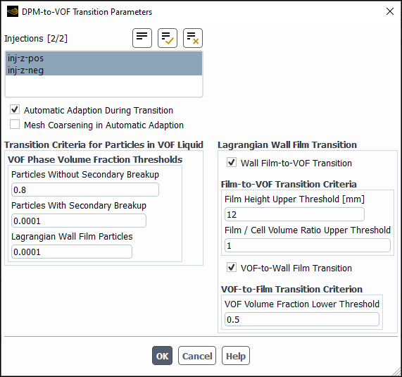
The tracking of a DPM particle is stopped as soon as the transition criteria are met, and the particle is scheduled for the model transition. All such particles are then transitioned into equivalent amounts of the selected VOF phase before the transport equation solver for the continuous phase is started for the current timestep.
The DPM-to-VOF model transition mechanism conserves mass and momentum of the transitioning phase regardless of the sizes of the particles and the cells. Particles that are much smaller than the cell are usually transitioned into the same cell, while particles that are larger than the cell are transitioned by introducing VOF liquid and removing equal amounts of VOF gas in multiple cells that form a hemispherically-shaped phase boundary around the location of the particle at the time when the model transition mechanism is triggered.
The figures below show changes in the gas-liquid interface and in the mesh in the process of the DPM-to-VOF model transition and automatic mesh adaption.
Figure 26.42: DPM Particles at the Gas-Liquid Interface displays a planar gas-liquid surface and three large Lagrangian DPM particles. The center points of the particles have just reached the phase boundary and the particles are about to be converted.
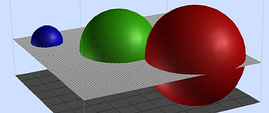
Figure 26.43: Surface Mesh Before the Model Transition is Triggered shows the surface mesh of the surrounding box. The phase boundary has been resolved by the solution-adaptive mesh refinement using appropriate criteria.
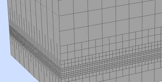
Figure 26.44: Gas-Liquid Interface after the Model Transition is Triggered shows the VOF phase interface right after the model transition has been triggered.
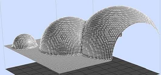
For the smallest particle, a hemisphere has been formed. Its volume is equal to that of the Lagrangian DPM particle. This includes the part of the particle that has already penetrated the VOF liquid.
The other two particles overlapped, which was neglected in the calculation of the particle trajectories. This has been taken into account by the DPM-to-VOF model transition mechanism to ensure total conservation of mass.
Figure 26.45: Surface Mesh After the Mesh Adaption and Phase Transition demonstrates the surface mesh of the same surrounding box as in Figure 26.43: Surface Mesh Before the Model Transition is Triggered after the DPM particles have been transitioned to VOF liquid. During the model transition, automatic adaption has been triggered as many times as necessary, so that the maximum mesh refinement has been reached, and the new gas-liquid boundary has been formed as a result. At the same time, the mesh coarsening has removed the mesh refinement in the location inside the large particle where an interface no longer exists after the model transition.
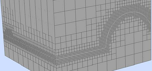
Note: The DPM-to-VOF model transition mechanism is independent of the phase materials. It may, therefore, be possible to apply the same model transition mechanism to scenarios with exchanged gas and liquid phases, for example, for gas bubbles modeled as Lagrangian DPM particles that reach a free liquid surface. However, no experience has been gathered with the application of this transition mechanism to such a scenario.
In addition, the volume-balancing approach would result in more recognizable mass losses in the liquid phase as VOF liquid would be removed and replaced by VOF gas wherever a Lagrangian DPM particle reaches the VOF gas-liquid interface. This may be appropriate if the process of displacing liquid by accumulating gas is to be modeled, but it is not acceptable, for example, for the analysis of a bubble column or an aerated stirred tank reactor where conservation of the liquid is expected.
For such applications, it is recommended to either approximate the free liquid surface with the No Slip shear condition and escape DPM wall boundary conditions or use a user-defined function to stop particle tracking for particles representing gas bubbles that have reached the free liquid surface.
In the current implementation of the DPM-to-VOF model transition, no splashing or any other kind of interaction between a droplet and a film or pool of liquid is considered. Whenever the center of a Lagrangian DPM particle reaches a cell that fulfills the applicable criteria, the amount of liquid represented by the particle is assumed to stick to the existing VOF liquid.
In addition to momentum and mass of the transitioning phase, heat and composition are also conserved. However, as explained above, in the Volume-Balancing Eulerian Phase, conservation of mass (or volume) and other quantities associated with the mass is not fulfilled.
The DPM-to-VOF model transition is not compatible with:
Steady-state flow
Steady particle tracking
2D Fluent mode
Eulerian multiphase model with Multi- Fluid VOF enabled
Shared-memory parallel DPM tracking
Use DPM Domain option of the Hybrid parallel DPM tracking mode