


Information about non-premixed combustion and mixture fraction theory are presented in the following sections:
The basis of the non-premixed modeling approach is that under
a certain set of simplifying assumptions, the instantaneous thermochemical
state of the fluid is related to a conserved scalar quantity known
as the mixture fraction,  . The mixture fraction can be written in terms of
the atomic mass fraction as [601]:
. The mixture fraction can be written in terms of
the atomic mass fraction as [601]:
 | (8–1) |
where  is the elemental mass fraction
for element,
is the elemental mass fraction
for element,  . The subscript ox denotes the
value at the oxidizer stream inlet and the subscript fuel denotes
the value at the fuel stream inlet. If the diffusion coefficients
for all species are equal, then Equation 8–1 is identical for all elements, and the mixture fraction definition
is unique. The mixture fraction is therefore the elemental mass fraction
that originated from the fuel stream.
. The subscript ox denotes the
value at the oxidizer stream inlet and the subscript fuel denotes
the value at the fuel stream inlet. If the diffusion coefficients
for all species are equal, then Equation 8–1 is identical for all elements, and the mixture fraction definition
is unique. The mixture fraction is therefore the elemental mass fraction
that originated from the fuel stream.
If a secondary stream (another fuel or oxidant, or a non-reacting stream) is included, the fuel and secondary mixture fractions are simply the elemental mass fractions of the fuel and secondary streams, respectively. The sum of all three mixture fractions in the system (fuel, secondary stream, and oxidizer) is always equal to 1:
 | (8–2) |
This indicates that only points on the plane ABC (shown in
Figure 8.1: Relationship of Mixture Fractions (Fuel, Secondary Stream,
and Oxidizer)) in the mixture fraction space
are valid. Consequently, the two mixture fractions,  and
and  , cannot vary independently; their values are valid
only if they are both within the triangle OBC shown in Figure 8.1: Relationship of Mixture Fractions (Fuel, Secondary Stream,
and Oxidizer).
, cannot vary independently; their values are valid
only if they are both within the triangle OBC shown in Figure 8.1: Relationship of Mixture Fractions (Fuel, Secondary Stream,
and Oxidizer).
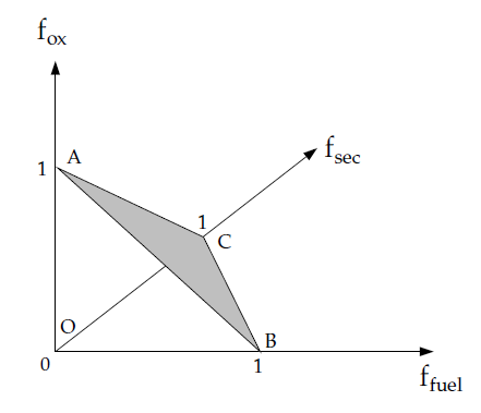
Figure 8.2: Relationship of Mixture Fractions (Fuel, Secondary Stream, and Normalized Secondary Mixture Fraction)
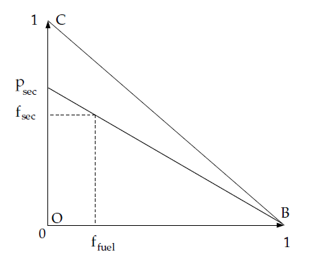
Ansys Fluent discretizes the triangle OBC as shown in Figure 8.2: Relationship of Mixture Fractions (Fuel, Secondary Stream,
and Normalized Secondary Mixture Fraction). Essentially, the primary mixture
fraction,  , is allowed to vary between zero and one, as for
the single mixture fraction case, while the secondary mixture fraction
lies on lines with the following equation:
, is allowed to vary between zero and one, as for
the single mixture fraction case, while the secondary mixture fraction
lies on lines with the following equation:
 | (8–3) |
where  is
the normalized secondary mixture fraction and is the value at the
intersection of a line with the secondary mixture fraction axis. Note
that unlike
is
the normalized secondary mixture fraction and is the value at the
intersection of a line with the secondary mixture fraction axis. Note
that unlike  ,
,  is bounded between zero and one, regardless of the
  value.
An important characteristic of the normalized secondary mixture
fraction,  ,
is its assumed statistical independence from the fuel mixture fraction,
,
is its assumed statistical independence from the fuel mixture fraction,  . Note that unlike
  ,
,  is
not a conserved scalar. This normalized mixture fraction definition,
is
not a conserved scalar. This normalized mixture fraction definition,  , is used everywhere in Ansys Fluent when prompted for
Secondary Mixture Fraction except when defining the rich limit for
a secondary fuel stream, which is defined in terms of
, is used everywhere in Ansys Fluent when prompted for
Secondary Mixture Fraction except when defining the rich limit for
a secondary fuel stream, which is defined in terms of  .
.
Under the assumption of equal diffusivities, the species equations
can be reduced to a single equation for the mixture fraction,  . The reaction source terms
in the species equations cancel (since elements are conserved in chemical
reactions), and therefore
. The reaction source terms
in the species equations cancel (since elements are conserved in chemical
reactions), and therefore  is a conserved quantity. While the assumption of
equal diffusivities is problematic for laminar flows, it is generally
acceptable for turbulent flows where turbulent convection overwhelms
molecular diffusion. The Favre mean (density-averaged) mixture fraction
equation is
is a conserved quantity. While the assumption of
equal diffusivities is problematic for laminar flows, it is generally
acceptable for turbulent flows where turbulent convection overwhelms
molecular diffusion. The Favre mean (density-averaged) mixture fraction
equation is
 | (8–4) |
where  is laminar thermal conductivity of the mixture,
  is the mixture specific heat,
  is the Prandtl number,
  is the turbulent viscosity,
  is the source term due solely to transfer of mass into the gas phase from
liquid fuel droplets or reacting particles (for example, coal), and
is the source term due solely to transfer of mass into the gas phase from
liquid fuel droplets or reacting particles (for example, coal), and  is any user-defined source term.
In addition to solving for the Favre mean mixture fraction, Ansys Fluent solves
a conservation equation for the mixture fraction variance,  [283]:
 | (8–5) |
where  is the turbulent kinetic energy, and
  . The default values for the constants
  ,
,  , and
, and  are 0.85, 2.86, and 2.0, respectively.
The mixture fraction variance is used in the closure model describing turbulence-chemistry interactions (see Modeling of Turbulence-Chemistry Interaction).
For a two-mixture-fraction problem,  and
and  are obtained from Equation 8–4 and Equation 8–5 by substituting
  for
for  and
and  for
for  .
.  is obtained from Equation 8–4 by substituting
  for
for  .
.  is then calculated using Equation 8–3, and
  is obtained by
solving Equation 8–5 with
is obtained by
solving Equation 8–5 with  substituted for
  . To a first-order approximation, the variances
in
. To a first-order approximation, the variances
in  and
and  are relatively
insensitive to
are relatively
insensitive to  , and therefore
the equation for
, and therefore
the equation for  is essentially the same as
  .
.
Important: The equation for  instead of
  is valid when
the mass flow rate of the secondary stream is relatively small compared
with the total mass flow rate.
is valid when
the mass flow rate of the secondary stream is relatively small compared
with the total mass flow rate.
For Large Eddy Simulations, the transport equation is not solved for the mixture fraction variance. Instead, it is modeled as
 | (8–6) |
| where | |
 = constant = constant | |
 = subgrid length scale (see Equation 4–307) = subgrid length scale (see Equation 4–307) |
The constant  is computed dynamically when the Dynamic
Stress option is enabled in the Viscous dialog box, else a constant value (with a default of 0.5) is used.
is computed dynamically when the Dynamic
Stress option is enabled in the Viscous dialog box, else a constant value (with a default of 0.5) is used.
If the Dynamic Scalar Flux option is enabled,
the turbulent Sc ( in Equation 8–4) is computed dynamically.
With the SBES turbulence model, clearly identifiable RANS and LES regions are present in the domain. When the transition from RANS to LES and vice versa occurs, the mixture fraction variance from the RANS formulation calculated using Equation 8–5 and the mixture fraction variance from the LES formulation modeled using Equation 8–6 will not recover the identical behavior. To ensure consistent transition between RANS and LES models, the transport equation of the mixture fraction variance is used in the RANS region, while the algebraic formulation is used in the LES region. The blending of the two is done in the same way as for turbulent viscosity (Equation 4–297). The mixture fraction variance for SBES is modeled as:
 | (8–7) |
The mixture fraction definition can be understood in relation to common measures of reacting systems. Consider a simple combustion system involving a fuel stream (F), an oxidant stream (O), and a product stream (P) symbolically represented at stoichiometric conditions as
 | (8–8) |
where  is the air-to-fuel ratio on a mass basis. Denoting
the equivalence ratio as
is the air-to-fuel ratio on a mass basis. Denoting
the equivalence ratio as  , where
 | (8–9) |
the reaction in Equation 8–8, under more general mixture conditions, can then be written as
 | (8–10) |
Looking at the left side of this equation, the mixture fraction for the system as a whole can then be deduced to be
 | (8–11) |
Equation 8–11 allows the computation
of the mixture fraction at stoichiometric conditions ( = 1) or at fuel-rich
conditions (for example,
= 1) or at fuel-rich
conditions (for example,  > 1),
or fuel-lean conditions (for example,
> 1),
or fuel-lean conditions (for example,  < 1).
< 1).
The power of the mixture fraction modeling approach is that the chemistry is reduced to one or two conserved mixture fractions. Under the assumption of chemical equilibrium, all thermochemical scalars (species fractions, density, and temperature) are uniquely related to the mixture fraction(s).
For a single mixture fraction in an adiabatic system, the instantaneous
values of mass fractions, density, and temperature depend solely on
the instantaneous mixture fraction,  :
:
 | (8–12) |
If a secondary stream is included, the instantaneous values
will depend on the instantaneous fuel mixture fraction,  , and the secondary partial
fraction,
, and the secondary partial
fraction,  :
:
 | (8–13) |
In Equation 8–12 and Equation 8–13,  represents
the instantaneous species mass fraction, density, or temperature.
In the case of non-adiabatic systems, the effect of heat loss/gain
is parameterized as
represents
the instantaneous species mass fraction, density, or temperature.
In the case of non-adiabatic systems, the effect of heat loss/gain
is parameterized as
 | (8–14) |
for a single mixture fraction system, where  is the instantaneous enthalpy
(see Equation 5–8).
is the instantaneous enthalpy
(see Equation 5–8).
If a secondary stream is included,
 | (8–15) |
Examples of non-adiabatic flows include systems with radiation, heat transfer through walls, heat transfer to/from discrete phase particles or droplets, and multiple inlets at different temperatures. Additional detail about the mixture fraction approach in such non-adiabatic systems is provided in Non-Adiabatic Extensions of the Non-Premixed Model.
In many reacting systems, the combustion is not in chemical equilibrium. Ansys Fluent offers several approaches to model chemical non-equilibrium, including the finite-rate (see The Generalized Finite-Rate Formulation for Reaction Modeling), EDC (see The Eddy-Dissipation-Concept (EDC) Model), and PDF transport (see Composition PDF Transport) models, where detailed kinetic mechanisms can be incorporated.
There are three approaches in the non-premixed combustion model to simulate chemical non-equilibrium. The first is to use the Rich Flammability Limit (RFL) option in the Equilibrium model, where rich regions are modeled as a mixed-but-unburnt mixture of pure fuel and a leaner equilibrium burnt mixture (see Enabling the Rich Flammability Limit (RFL) Option in the User’s Guide). The second approach is the Steady Diffusion Flamelet model, where chemical non-equilibrium due to diffusion flame stretching by turbulence can be modeled. The third approach is the Unsteady Diffusion Flamelet model where slow-forming product species that are far from chemical equilibrium can be modeled. See The Diffusion Flamelet Models Theory and The Unsteady Diffusion Flamelet Model Theory for details about the Steady and Unsteady Diffusion Flamelet models in Ansys Fluent.
Equation 8–12 through Equation 8–15 describe the instantaneous relationships between mixture fraction and species fractions, density, and temperature under the assumption of chemical equilibrium. The Ansys Fluent prediction of the turbulent reacting flow, however, is concerned with prediction of the averaged values of these fluctuating scalars. How these averaged values are related to the instantaneous values depends on the turbulence-chemistry interaction model. Ansys Fluent applies the assumed-shape probability density function (PDF) approach as its closure model when the non-premixed model is used. The assumed shape PDF closure model is described in this section.
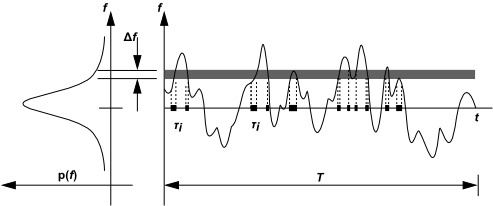
The Probability Density Function, written as  , can be
thought of as the fraction of time that the fluid spends in the vicinity
of the state
, can be
thought of as the fraction of time that the fluid spends in the vicinity
of the state  . Figure 8.3: Graphical Description of the Probability Density Function plots
the time trace of mixture fraction at a point in the flow (right-hand
side) and the probability density function of
. Figure 8.3: Graphical Description of the Probability Density Function plots
the time trace of mixture fraction at a point in the flow (right-hand
side) and the probability density function of  (left-hand side). The fluctuating
value of
(left-hand side). The fluctuating
value of  , plotted on the right side of the figure, spends
some fraction of time in the range denoted as
, plotted on the right side of the figure, spends
some fraction of time in the range denoted as  .
.  , plotted
on the left side of the figure, takes on values such that the area
under its curve in the band denoted,
, plotted
on the left side of the figure, takes on values such that the area
under its curve in the band denoted,  , is equal
to the fraction of time that
, is equal
to the fraction of time that  spends in this range. Written mathematically,
 | (8–16) |
where  is the time scale and
  is the amount
of time that
is the amount
of time that  spends in the
  band. The shape of the function
 depends on the nature of the turbulent
fluctuations in
depends on the nature of the turbulent
fluctuations in  . In practice,
  is unknown and is modeled as a
mathematical function that approximates the actual PDF shapes that
have been observed experimentally.
is unknown and is modeled as a
mathematical function that approximates the actual PDF shapes that
have been observed experimentally.
The probability density function  , describing
the temporal fluctuations of
, describing
the temporal fluctuations of  in the turbulent flow, can be used to compute averaged
values of variables that depend on
in the turbulent flow, can be used to compute averaged
values of variables that depend on  . Density-weighted mean species
mass fractions and temperature can be computed (in adiabatic systems)
as
. Density-weighted mean species
mass fractions and temperature can be computed (in adiabatic systems)
as
 | (8–17) |
for a single-mixture-fraction system. When a secondary stream exists, mean values are calculated as
 | (8–18) |
where  is the PDF
of
is the PDF
of  and
and  is the PDF
of
is the PDF
of  .
Here, statistical independence of
.
Here, statistical independence of  and
and  is
assumed, so that
is
assumed, so that  .
.
Similarly, the mean time-averaged fluid density,  , can be computed as
 | (8–19) |
for a single-mixture-fraction system, and
 | (8–20) |
when a secondary stream exists.  or
or  is the instantaneous
density obtained using the instantaneous species mass fractions and
temperature in the ideal gas law equation.
is the instantaneous
density obtained using the instantaneous species mass fractions and
temperature in the ideal gas law equation.
Using Equation 8–17 and Equation 8–19 (or Equation 8–18 and Equation 8–20), it remains only
to specify the shape of the function  (or
(or  and
and  ) in order to determine the local mean fluid
state at all points in the flow field.
) in order to determine the local mean fluid
state at all points in the flow field.
The shape of the assumed PDF,  , is described
in Ansys Fluent by one of two mathematical functions:
, is described
in Ansys Fluent by one of two mathematical functions:
the double-delta function (two-mixture-fraction cases only)
the
 -function (single- and two-mixture-fraction
cases)
-function (single- and two-mixture-fraction
cases)
The double-delta function is the most easily computed, while
the  -function most closely represents experimentally
observed PDFs. The shape produced by this function depends solely
on the mean mixture fraction,
-function most closely represents experimentally
observed PDFs. The shape produced by this function depends solely
on the mean mixture fraction,  , and its variance,
  . A detailed description
of each function follows.
. A detailed description
of each function follows.
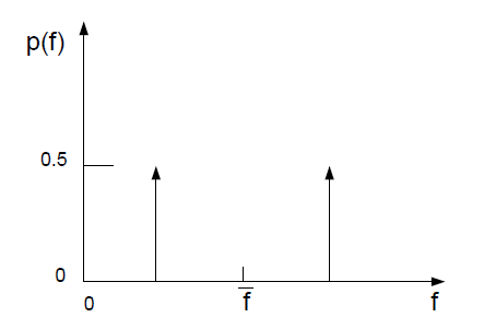
The double delta function is given by
 | (8–21) |
with suitable bounding near  = 1 and
  = 0. One example of the double
delta function is illustrated in Figure 8.4: Example of the Double Delta Function PDF Shape. As noted above, the double delta function PDF is very easy to
compute but is invariably less accurate than the alternate
= 0. One example of the double
delta function is illustrated in Figure 8.4: Example of the Double Delta Function PDF Shape. As noted above, the double delta function PDF is very easy to
compute but is invariably less accurate than the alternate  -function PDF because
it assumes that only two states occur in the turbulent flow. For this
reason, it is available only for two-mixture-fraction simulations
where the savings in computational cost is significant.
-function PDF because
it assumes that only two states occur in the turbulent flow. For this
reason, it is available only for two-mixture-fraction simulations
where the savings in computational cost is significant.
The  -function PDF shape is given by the following
function of
-function PDF shape is given by the following
function of  and
and  :
:
 | (8–22) |
where
 | (8–23) |
and
 | (8–24) |
Importantly, the PDF shape  is a function
of only its first two moments, namely the mean mixture fraction,
is a function
of only its first two moments, namely the mean mixture fraction,  , and the mixture fraction variance,
  . Thus, given Ansys Fluent’s
prediction of
. Thus, given Ansys Fluent’s
prediction of  and
and  at each point in the flow field (Equation 8–4 and Equation 8–5), the assumed PDF shape can
be computed and used as the weighting function to determine the mean
values of species mass fractions, density, and temperature using,
Equation 8–17 and Equation 8–19 (or, for a system with
a secondary stream, Equation 8–18 and Equation 8–20).
at each point in the flow field (Equation 8–4 and Equation 8–5), the assumed PDF shape can
be computed and used as the weighting function to determine the mean
values of species mass fractions, density, and temperature using,
Equation 8–17 and Equation 8–19 (or, for a system with
a secondary stream, Equation 8–18 and Equation 8–20).
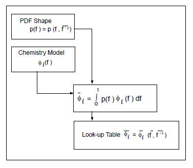
This logical dependence is depicted visually in Figure 8.5: Logical Dependence of Averaged Scalars on Mean Mixture Fraction, the Mixture Fraction Variance, and the Chemistry Model (Adiabatic, Single-Mixture-Fraction Systems) for a single mixture fraction.
Figure 8.5: Logical Dependence of Averaged Scalars on Mean Mixture Fraction, the Mixture Fraction Variance, and the Chemistry Model (Adiabatic, Single-Mixture-Fraction Systems)
Many reacting systems involve heat transfer through wall boundaries,
droplets, and/or particles. In such flows the local thermochemical
state is no longer related only to  , but also to the enthalpy,
  . The system enthalpy impacts
the chemical equilibrium calculation and the temperature and species
of the reacting flow. Consequently, changes in enthalpy due to heat
loss must be considered when computing scalars from the mixture fraction,
as in Equation 8–14.
. The system enthalpy impacts
the chemical equilibrium calculation and the temperature and species
of the reacting flow. Consequently, changes in enthalpy due to heat
loss must be considered when computing scalars from the mixture fraction,
as in Equation 8–14.
In such non-adiabatic systems, turbulent fluctuations should
be accounted for by means of a joint PDF,  . The computation of
  , however, is not practical
for most engineering applications. The problem can be simplified significantly
by assuming that the enthalpy fluctuations are independent of the
enthalpy level (that is, heat losses do not significantly impact the
turbulent enthalpy fluctuations). With this assumption,
, however, is not practical
for most engineering applications. The problem can be simplified significantly
by assuming that the enthalpy fluctuations are independent of the
enthalpy level (that is, heat losses do not significantly impact the
turbulent enthalpy fluctuations). With this assumption,  and mean scalars are calculated as
 | (8–25) |
Determination of  in the non-adiabatic system therefore requires solution
of the modeled transport equation for mean enthalpy:
in the non-adiabatic system therefore requires solution
of the modeled transport equation for mean enthalpy:
 | (8–26) |
where  accounts for source terms due
to radiation, heat transfer to wall boundaries, and heat exchange
with the dispersed phase.
accounts for source terms due
to radiation, heat transfer to wall boundaries, and heat exchange
with the dispersed phase.
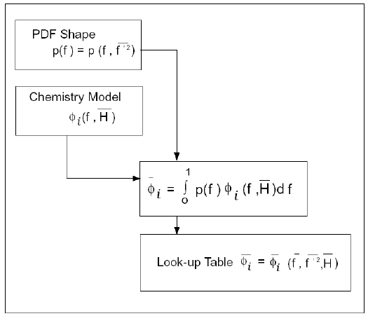
Figure 8.6: Logical Dependence of Averaged Scalars on Mean Mixture Fraction,
the Mixture Fraction Variance, Mean Enthalpy, and the Chemistry Model
(Non-Adiabatic, Single-Mixture-Fraction Systems) depicts
the logical dependence of mean scalar values (species mass fraction,
density, and temperature) on Ansys Fluent’s prediction of  ,
,  , and
, and  in non-adiabatic single-mixture-fraction
systems.
in non-adiabatic single-mixture-fraction
systems.
Figure 8.6: Logical Dependence of Averaged Scalars on Mean Mixture Fraction, the Mixture Fraction Variance, Mean Enthalpy, and the Chemistry Model (Non-Adiabatic, Single-Mixture-Fraction Systems)
When a secondary stream is included, the mean values are calculated from
 | (8–27) |
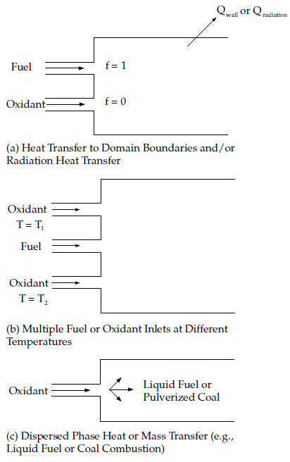
As noted above, the non-adiabatic extensions to the PDF model are required in systems involving heat transfer to walls and in systems with radiation included. In addition, the non-adiabatic model is required in systems that include multiple fuel or oxidizer inlets with different inlet temperatures. Finally, the non-adiabatic model is required in particle-laden flows (for example, liquid fuel systems or coal combustion systems) when such flows include heat transfer to the dispersed phase. Figure 8.7: Reacting Systems Requiring Non-Adiabatic Non-Premixed Model Approach illustrates several systems that must include the non-adiabatic form of the PDF model.
For an equilibrium, adiabatic, single-mixture-fraction case,
the mean temperature, density, and species fraction are functions
of the  and
and  only (see Equation 8–17 and Equation 8–22). Significant computational time
can be saved by computing these integrals once, storing them in a
look-up table, and retrieving them during the Ansys Fluent simulation.
only (see Equation 8–17 and Equation 8–22). Significant computational time
can be saved by computing these integrals once, storing them in a
look-up table, and retrieving them during the Ansys Fluent simulation.
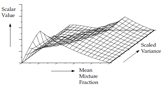
Figure 8.8: Visual Representation of a Look-Up Table for the Scalar (Mean
Value of Mass Fractions, Density, or Temperature) as a Function of
Mean Mixture Fraction and Mixture Fraction Variance in Adiabatic Single-Mixture-Fraction
Systems illustrates the
concept of the look-up tables generated for a single-mixture-fraction
system. Given Ansys Fluent’s predicted value for  and
and  at a point in
the flow domain, the mean value of mass fractions, density, or temperature
(
at a point in
the flow domain, the mean value of mass fractions, density, or temperature
( ) at that point can be obtained by table interpolation.
The table, Figure 8.8: Visual Representation of a Look-Up Table for the Scalar (Mean Value of Mass Fractions, Density, or Temperature) as a Function of Mean Mixture Fraction and Mixture Fraction Variance in Adiabatic Single-Mixture-Fraction Systems, is the mathematical result of the integration of Equation 8–17. There is one look-up table of this type for each scalar of interest (species mass fractions, density, and temperature). In adiabatic systems, where the instantaneous enthalpy is a function of only the instantaneous mixture fraction, a two-dimensional look-up table, like that in Figure 8.8: Visual Representation of a Look-Up Table for the Scalar (Mean Value of Mass Fractions, Density, or Temperature) as a Function of Mean Mixture Fraction and Mixture Fraction Variance in Adiabatic Single-Mixture-Fraction Systems, is all that is required.
Figure 8.8: Visual Representation of a Look-Up Table for the Scalar (Mean Value of Mass Fractions, Density, or Temperature) as a Function of Mean Mixture Fraction and Mixture Fraction Variance in Adiabatic Single-Mixture-Fraction Systems
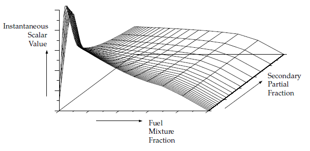
For systems with two mixture fractions, the creation and interpolation
costs of four-dimensional look-up tables are computationally expensive.
By default, the instantaneous properties  are tabulated
as a function of the fuel mixture fraction
are tabulated
as a function of the fuel mixture fraction  and the secondary partial fraction
  (see Equation 8–13),
and the PDF integrations (see Equation 8–15) are performed at run time.
This two-dimensional table is illustrated in Figure 8.9: Visual Representation of a Look-Up Table for the Scalar φ_I
as a Function of Fuel Mixture Fraction and Secondary Partial Fraction
in Adiabatic Two-Mixture-Fraction Systems. Alternatively, 4D look-up
tables can be created before the simulation and interpolated at run
time (see Full Tabulation of the Two-Mixture-Fraction Model in the User's
Guide).
(see Equation 8–13),
and the PDF integrations (see Equation 8–15) are performed at run time.
This two-dimensional table is illustrated in Figure 8.9: Visual Representation of a Look-Up Table for the Scalar φ_I
as a Function of Fuel Mixture Fraction and Secondary Partial Fraction
in Adiabatic Two-Mixture-Fraction Systems. Alternatively, 4D look-up
tables can be created before the simulation and interpolated at run
time (see Full Tabulation of the Two-Mixture-Fraction Model in the User's
Guide).
Figure 8.9: Visual Representation of a Look-Up Table for the Scalar φ_I as a Function of Fuel Mixture Fraction and Secondary Partial Fraction in Adiabatic Two-Mixture-Fraction Systems
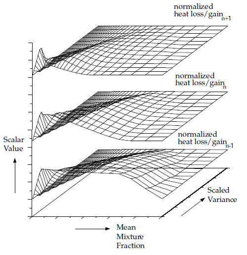
In non-adiabatic systems, where the enthalpy is not linearly related to the mixture fraction, but depends also on wall heat transfer and/or radiation, a look-up table is required for each possible enthalpy value in the system. The result, for single mixture fraction systems, is a three-dimensional look-up table, as illustrated in Figure 8.10: Visual Representation of a Look-Up Table for the Scalar as a Function of Mean Mixture Fraction and Mixture Fraction Variance and Normalized Heat Loss/Gain in Non-Adiabatic Single-Mixture-Fraction Systems, which consists of layers of two-dimensional tables, each one corresponding to a normalized heat loss or gain. The first slice corresponds to the maximum heat loss from the system, the last slice corresponds to the maximum heat gain to the system, and the zero heat loss/gain slice corresponds to the adiabatic table. Slices interpolated between the adiabatic and maximum slices correspond to heat gain, and those interpolated between the adiabatic and minimum slices correspond to heat loss.
The three-dimensional look-up table allows Ansys Fluent to determine
the value of each mass fraction, density, and temperature from calculated
values of  ,
,  , and
, and  . This three-dimensional table in Figure 8.10: Visual Representation of a Look-Up Table for the Scalar as
a Function of Mean Mixture Fraction and Mixture Fraction Variance
and Normalized Heat Loss/Gain in Non-Adiabatic Single-Mixture-Fraction
Systems is the visual representation
of the integral in Equation 8–25.
. This three-dimensional table in Figure 8.10: Visual Representation of a Look-Up Table for the Scalar as
a Function of Mean Mixture Fraction and Mixture Fraction Variance
and Normalized Heat Loss/Gain in Non-Adiabatic Single-Mixture-Fraction
Systems is the visual representation
of the integral in Equation 8–25.
Figure 8.10: Visual Representation of a Look-Up Table for the Scalar as a Function of Mean Mixture Fraction and Mixture Fraction Variance and Normalized Heat Loss/Gain in Non-Adiabatic Single-Mixture-Fraction Systems
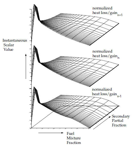
For non-adiabatic, two-mixture-fraction problems, it is very expensive to tabulate and retrieve Equation 8–27 since five-dimensional tables are required. By default, 3D lookup tables of the instantaneous state relationship given by Equation 8–15 are created. The 3D table in Figure 8.11: Visual Representation of a Look-Up Table for the Scalar φ_I as a Function of Fuel Mixture Fraction and Secondary Partial Fraction, and Normalized Heat Loss/Gain in Non-Adiabatic Two-Mixture-Fraction Systems is the visual representation of Equation 8–15. The mean density during the Ansys Fluent solution is calculated by integrating the instantaneous density over the fuel and secondary mixture fraction space (see Equation 8–27). Alternatively, 5D look-up tables can be created before the simulation and interpolated at run time (see Full Tabulation of the Two-Mixture-Fraction Model in the User's Guide). The one-time pre-generation of the 5D look-up table is very expensive, but, once built, interpolating the table during an Ansys Fluent solution is usually significantly faster than performing the integrations at run time. This is especially true for cases with a large number of cells that require many iterations or time steps to converge.
Important: Note that the computation time in Ansys Fluent for a two-mixture-fraction case will be much greater than for a single-mixture-fraction problem. This expense should be carefully considered before choosing the two-mixture-fraction model. Also, it is usually expedient to start a two-mixture-fraction simulation from a converged single-mixture-fraction solution.
Figure 8.11: Visual Representation of a Look-Up Table for the Scalar φ_I as a Function of Fuel Mixture Fraction and Secondary Partial Fraction, and Normalized Heat Loss/Gain in Non-Adiabatic Two-Mixture-Fraction Systems
Ansys Fluent has the capability of generating lookup tables using Automated Grid Refinement. The adaptive algorithm inserts grid points in all table dimensions so that changes in values of tabulated variables (such as mean temperature, density, and species mass fractions) between successive grid points as well as changes in their slopes are less than a user-specified tolerance. The advantage of automated grid refinement is that tabulated quantities are resolved only in regions of rapid change. Therefore, compared to a fixed grid, more accurate and/or smaller PDF tables will be generated.
When using automated grid refinement, table points are calculated on a coarse grid with a user
specified Initial Number of Grid Points (default of 15). A new grid point
is inserted midway between a point  and its neighbor
  if,
if,
 | (8–28) |
where  is the value of a table variable at grid point
  ,
,  is a user specified Maximum Change in Value Ratio
(default of 0.25), and
is a user specified Maximum Change in Value Ratio
(default of 0.25), and  (
( ) are the maximum (minimum) table values over all grid points.
In addition to ensuring gradual change in value between successive table points, a grid point is added if
 | (8–29) |
where the slope at any point  is defined
as,
is defined
as,
 | (8–30) |
In Equation 8–29 and Equation 8–30,  is a user specified Maximum Change in Slope Ratio
(default of 0.25),
is a user specified Maximum Change in Slope Ratio
(default of 0.25),  (
( ) are the maximum (minimum) slopes over all grid points, and
  is the value of the independent grid variable being refined (that is, mean
mixture fraction, mixture fraction variance or mean enthalpy).
is the value of the independent grid variable being refined (that is, mean
mixture fraction, mixture fraction variance or mean enthalpy).
The automated grid refinement algorithm is summarized as follows: an initial grid in the mean mixture fraction dimension is created with the specified Initial Number of Grid Points. Grid points are then inserted when the change in table mean temperature, and mean H2, CO and OH mole fractions, between two grid points, or the change in their slope between three grid points, is more than what you specified in Maximum Change in Value/Slope Ratio. This process is repeated until all points satisfy the specified value and slope change requirements, or the Maximum Number of Grid Points is exceeded. This procedure is then repeated for the mixture fraction variance dimension, which is calculated at the mean stoichiometric mixture fraction. Finally, if the non-adiabatic option is enabled, the procedure is repeated for the mean enthalpy grid, evaluated at the mean stoichiometric mixture fraction and zero mixture fraction variance.
When steady diffusion flamelets are used, the Automated Grid Refinement can generate different mean mixture fraction grid points than specified in the diffusion flamelets. For such cases, a 4th order polynomial interpolation is used to obtain the flamelet solution at the inserted points.
Note: The second order interpolation option is faster than fourth order interpolation, especially for tables with high dimensions, such as non-adiabatic flamelets. However, under-resolved tables that are interpolated with second order can lead to convergence difficulties. Therefore, the Automated Grid Refinement (AGR) option places grid points optimally when generating PDF tables. Hence, AGR should be used in general, and especially for second order interpolation.
Note: Automated grid refinement is not available with two mixture fractions.
For more information about the input parameters used to generate lookup tables, refer to Calculating the Look-Up Tables in the User's Guide.