The Ffowcs Williams and Hawkings (FW-H) equation is essentially an inhomogeneous wave equation that can be derived by manipulating the continuity equation and the Navier-Stokes equations. The FW-H  [79] , [178] equation can be written as:

(11–1)

is the sound pressure at the far field ( ). denotes a mathematical surface introduced to "embed" the exterior flow problem ( ) in an unbounded space, which facilitates the use of generalized function theory and the free-space Green function to obtain the solution. The surface ( ) corresponds to the source (emission) surface, and can be made coincident with a body (impermeable) surface or a permeable surface off the body surface. is the unit normal vector pointing toward the exterior region ( ), is the far-field sound speed, and is the Lighthill stress tensor, defined as

(11–2)

is the compressive stress tensor. For a Stokesian fluid, this is given by

(11–3)

The free-stream quantities are denoted by the subscript .

The wave equation Equation 11–1 can be integrated analytically under the assumptions of the free-space flow and the absence of obstacles between the sound sources and the receivers. The complete solution consists of surface integrals and volume integrals. The surface integrals represent the contributions from monopole and dipole acoustic sources and partially from quadrupole sources, whereas the volume integrals represent quadrupole (volume) sources in the region outside the source surface. The contribution of the volume integrals becomes small when the flow is low subsonic and the source surface encloses the source region. In Ansys Fluent, the volume integrals are dropped. Thus, we have

(11–4)

where

(11–5)

(11–6)

where

(11–7)

(11–8)

When the integration surface coincides with an impenetrable wall, the two terms on the right in Equation 11–4 , and , are often referred to as thickness and loading terms, respectively, in light of their physical meanings. The square brackets in Equation 11–5 and Equation 11–6 denote that the kernels of the integrals are computed at the corresponding retarded times, , defined as follows, given the receiver time, , and the distance to the receiver, ,

(11–9)

The various subscripted quantities appearing in Equation 11–5 and Equation 11–6 are the inner products of a vector and a unit vector implied by the subscript. For instance, and , where and denote the unit vectors in the radiation and wall-normal directions, respectively. The Mach number vector in Equation 11–5 and Equation 11–6 relates to the motion of the integration surface: . The quantity is a scalar product . The dot over a variable denotes source-time differentiation of that variable.

For the calculation of the aerodynamic sound caused by external flow around a body, the Convective Effects option must be enabled (see Setting Model Constants in the User's Guide ) with the far-field fluid velocity vector to be additionally specified. This option is relevant to practical situations such as the flight tests (microphones mounted on an airplane) or wind tunnel measurements (microphones mounted within the wind tunnel core flow region).

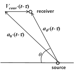
With the convective effects taken into account, the retarded time calculation becomes more complicated than the simple form of Equation 11–9 . As illustrated in Figure 11.1: Schematic of the Convective Effect on the Retarded Time Calculation , the effective sound propagation velocity is lower than in the upstream hemisphere and higher than in the downstream hemisphere, where is the direction angle towards the receiver counted from the upstream direction. According to Figure 11.1: Schematic of the Convective Effect on the Retarded Time Calculation the retarded time with the convective effect must be computed as

(11–10)

An obvious limitation for the Convective Effects option is that the far-field convection must be subsonic

Figure 11.1: Schematic of the Convective Effect on the Retarded Time Calculation

Note the following remarks regarding the applicability of the FW-H integral solution: