


Information about radiation modeling is presented in the following sections:
- 16.3.1. Using the Radiation Models
- 16.3.2. Setting Up the P-1 Model with Non-Gray Radiation
- 16.3.3. Setting Up the DTRM
- 16.3.4. Setting Up the S2S Model
- 16.3.5. Setting Up the DO Model
- 16.3.6. Setting Up the MC Model
- 16.3.7. Defining Material Properties for Radiation
- 16.3.8. Defining Boundary Conditions for Radiation
- 16.3.9. Solution Strategies for Radiation Modeling
- 16.3.10. Postprocessing Radiation Quantities
- 16.3.11. Solar Load Model
For theoretical information about the radiation models in Ansys Fluent, refer to Modeling Radiation in the Theory Guide.
The procedure for setting up and solving a radiation problem is outlined below, and described in detail in referenced sections. Steps that are relevant only for a particular radiation model are noted as such. The steps that are pertinent to radiation modeling, are shown here. For information about inputs related to other models that you are using in conjunction with radiation, see the appropriate sections for those models.
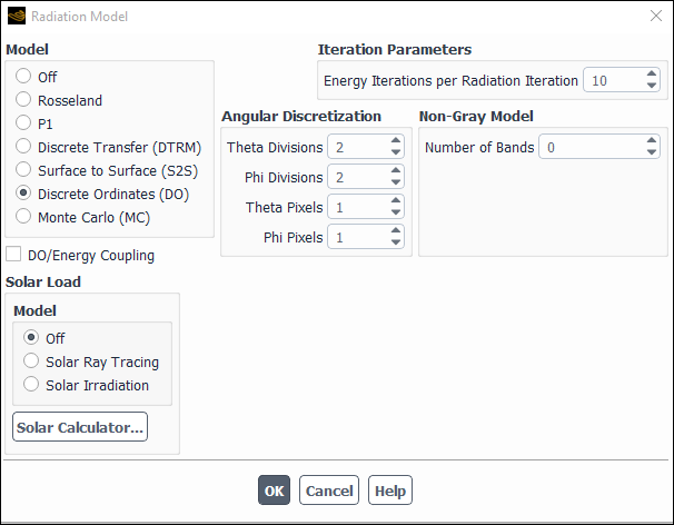
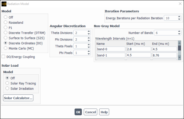
Enable radiative heat transfer by selecting a radiation model (Rosseland, P1, Discrete Transfer (DTRM), Surface to Surface (S2S), Discrete Ordinates, or Monte Carlo (MC)) under Model in the Radiation Model dialog box (Figure 16.16: The Radiation Model Dialog Box (DO Model)).
 Setup →
Models → Radiation
Setup →
Models → Radiation
 Edit...
Important: The Rosseland model can be used only with the pressure-based solver.
Note that when the P-1, the DTRM, the S2S, DO, or MC model is enabled, the Radiation Model dialog box expands to show additional parameters. These parameters will not appear if you select the Rosseland model. If you are running a 3D case, you will have the added option of using the solar load model. The solar load options will be displayed in the dialog box, below the radiation model settings.
When the radiation model is active, the radiation fluxes will be included in the solution of the energy equation at each iteration. If you set up a problem with the radiation model turned on, and you then decide to turn it off completely, you must select the button in the Radiation Model dialog box.
Note that when you enable a radiation model, Ansys Fluent will automatically enable the energy equation so that step is not needed.
Set the appropriate radiation parameters.
If you are modeling non-gray radiation using the P-1 model, define the non-gray radiation parameters as described in Setting Up the P-1 Model with Non-Gray Radiation.
If you are using the DTRM, define the ray tracing as described in Setting Up the DTRM.
If you are using the S2S model, define the surface clusters and view factors settings and compute or read the view factors as described in Setting Up the S2S Model.
If you are using the DO model, choose DO/Energy Coupling if desired, define the angular discretization as described in Setting Up the DO Model and, if relevant, define the non-gray radiation parameters as described in Defining Non-Gray Radiation for the DO Model.
If you are using the MC model, specify the Target Number of Histories as described in Setting Up the MC Model and, if relevant, similar to when using the DO model, define the non-gray radiation parameters as described in Defining Non-Gray Radiation for the DO Model.
Define the material properties as described in Defining Material Properties for Radiation.
Define the boundary conditions as described in Defining Boundary Conditions for Radiation. If your model contains a semi-transparent medium, see the information below on setting up semi-transparent media.
Set the parameters that control the solution (DTRM, DO, MC, S2S, and P-1 only) as described in Solution Strategies for Radiation Modeling.
Run the solution as described in Running the Calculation.
Postprocess the results as described in Postprocessing Radiation Quantities.
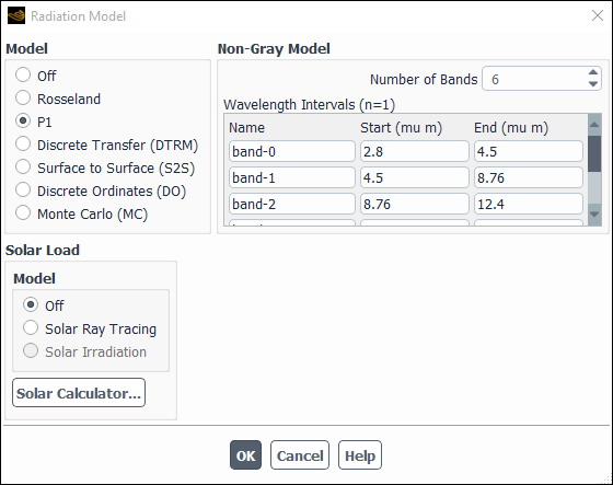
If you want to model non-gray radiation using the P-1 model, you can specify the
Number of Bands under Non-Gray Model
in the expanded Radiation Model dialog box (Figure 16.17: The Radiation Model Dialog Box (Non-Gray P-1 Model)). By default, the Number of
Bands is set to zero, indicating that only gray radiation will be
modeled. Because the cost of computation increases directly with the number of
bands, you should try to minimize the number of bands used. When a nonzero
Number of Bands is specified, the Radiation
Model dialog box will expand once again to show the
Wavelength Intervals. For each wavelength band, you can
specify a Name, as well as the Start and
End wavelength of the band in  m. Note that the wavelength bands are specified for vacuum
(
m. Note that the wavelength bands are specified for vacuum
( ). For more information about non-gray radiation calculations, see
Defining Non-Gray Radiation for the DO Model.
). For more information about non-gray radiation calculations, see
Defining Non-Gray Radiation for the DO Model.
Ansys Fluent allows you to use a user-defined function (UDF) to modify the
emissivity weighting factor  (which otherwise defaults to the black body emission factor
obtained from a standard Planck distribution). The emissivity weighting factor
appears in the emission term of the radiative transfer equation for the non-gray
model, as shown in Equation 5–64
in the Theory Guide. For more
information, see the Fluent Customization Manual.
(which otherwise defaults to the black body emission factor
obtained from a standard Planck distribution). The emissivity weighting factor
appears in the emission term of the radiative transfer equation for the non-gray
model, as shown in Equation 5–64
in the Theory Guide. For more
information, see the Fluent Customization Manual.
For information about setting up the DTRM, see the following sections:
When you select the Discrete Transfer model and click in the Radiation Model dialog box, the DTRM Rays dialog box (Figure 16.18: The DTRM Rays Dialog Box) will open automatically. If you need to modify the current settings later in the problem setup or solution procedure, you can open this dialog box by clicking in the Physics ribbon tab (Model Specific group box).
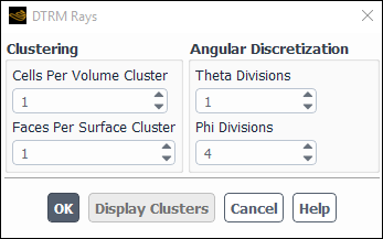
In this dialog box you will set parameters for and create the rays and clusters discussed in The DTRM Equations in the Theory Guide.
The procedure is as follows:
To control the number of radiating surfaces and absorbing cells, set the Cells Per Volume Cluster and Faces Per Surface Cluster. (See the explanation below.)
To control the number of rays being traced, set the number of Theta Divisions and Phi Divisions. (Guidelines are provided below.)
When you click in the DTRM Rays dialog box, The Select File Dialog Box will open prompting you for the name of the “ray file”. After you have specified the filename and chosen whether to write a binary ray file, Ansys Fluent will write the ray file and then read it afterward. During the write process the status of the DTRM ray tracing will be reported in the Ansys Fluent console. For example:
 Completed 25% tracing of DTRM rays

 Completed 50% tracing of DTRM rays

 Completed 75% tracing of DTRM rays

 Completed 100 % tracing of DTRM rays
See following sections for details on DTRM Rays dialog box inputs.
Important: If you cancel the DTRM Rays dialog box without writing and reading the ray file, the DTRM will be disabled.
Your inputs for Cells Per Volume Cluster and Faces Per Surface Cluster will control the number of radiating surfaces and absorbing cells. By default, each is set to 1, so the number of surface clusters (radiating surfaces) will be the number of boundary faces, and the number of volume clusters (absorbing cells) will be the number of cells in the domain. For small 2D problems, these are acceptable numbers, but for larger problems you will want to reduce the number of surface and/or volume clusters in order to reduce the ray-tracing expense. See Clustering in the Theory Guide for details about clustering.
Note:
Only zones attached to fluid cell zones are used for creating surface clusters.
Faces Per Surface Cluster (FPSC) is indicative of the actual reduction factor except when the surfaces are planar. The surface clustering algorithm uses other criteria (angle between faces, and so on) to ensure the clusters are nearly planar, so it is possible that there will be no further reduction in the total number of clusters beyond a certain value of FPSC.
Your inputs for Theta Divisions and Phi Divisions will control the number of rays being traced from each surface cluster (radiating surface).
Theta Divisions defines the number of discrete divisions in
the angle  used to define the solid angle about a point
  on a surface. The solid angle is defined as
  varies from 0 to 90 degrees (in the Theory Guide), and the default setting of 1 for
the number of discrete settings implies that there will be one ray traced from
the surface.
varies from 0 to 90 degrees (in the Theory Guide), and the default setting of 1 for
the number of discrete settings implies that there will be one ray traced from
the surface.
Phi Divisions defines the number of discrete divisions in
the angle  used to define the solid angle about a point
  on a surface. The solid angle is defined as
  varies from 0 to 360 degrees (Figure 5.2: Angles θ and φ Defining the Hemispherical Solid Angle
About a Point P in the Theory Guide). The default setting of 4 implies
that each ray traced from the surface will be located at a
90° angle, and in combination with the
default setting for Theta Divisions, above, implies that 4
rays will be traced from each surface control volume. In many cases, it is
recommended that you at least double the number of divisions in
varies from 0 to 360 degrees (Figure 5.2: Angles θ and φ Defining the Hemispherical Solid Angle
About a Point P in the Theory Guide). The default setting of 4 implies
that each ray traced from the surface will be located at a
90° angle, and in combination with the
default setting for Theta Divisions, above, implies that 4
rays will be traced from each surface control volume. In many cases, it is
recommended that you at least double the number of divisions in  and
and  .
.
After you have activated the DTRM and defined all of the parameters controlling the ray tracing, you must create a ray file, which will be read back in and used during the radiation calculation. The ray file contains a description of the ray traces (for example, path lengths, cells traversed by each ray). This information is stored in the ray file, instead of being recomputed, in order to speed up the calculation process.
By default, a binary ray file will be written. You can also create text (formatted) ray files by turning off the Write Binary Files option in The Select File Dialog Box.
Important: Do not write or read a compressed ray file, because Ansys Fluent will not be able to access the ray tracing information properly from a compressed ray file.
The ray filename must be specified to Ansys Fluent only once. Thereafter, the filename is stored in your case file and the ray file will be automatically read into Ansys Fluent whenever the case file is read. Ansys Fluent will remind you that it is reading the ray file after it finishes reading the rest of the case file by reporting its progress in the console.
Note that the ray filename stored in your case file may not contain the full name of the directory in which the ray file exists. The full directory name will be stored in the case file only if you initially read the ray file through the GUI (or if you typed in the directory name along with the filename when using the text interface). In the event that the full directory name is absent, the automatic reading of the ray file may fail (since Ansys Fluent does not know in which directory to look for the file), and you will need to manually specify the ray file, using the File/Read/DTRM Rays... ribbon tab item. The safest approaches are to use the GUI when you first read the ray file or to supply the full directory name when using the text interface.
Important: You must recreate the ray file whenever you do anything that changes the mesh, such as:
change the type of a boundary zone
adapt the mesh
scale the mesh
You can open the DTRM Rays dialog box directly by clicking in the Physics ribbon tab (Model Specific group box).
Once a ray file has been created or read in manually, you can click the button in the DTRM Rays dialog box to graphically display the clusters in the domain. See Displaying Rays and Clusters for the DTRM for additional information about displaying rays and clusters.
When you select the Surface to Surface (S2S) model, the Radiation Model dialog box will expand to show additional parameters (see Figure 16.19: The Radiation Model Dialog Box (S2S Model)). In these additional group boxes, you will set the solution parameters (see S2S Solution Parameters for further details), access the view factors and clustering settings, and compute the view factors for your problem or read previously computed view factors into Ansys Fluent.
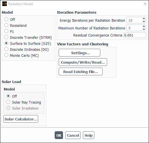
The S2S radiation model is very expensive in terms of computation effort and memory requirements when there are a large number of radiating surfaces. You can reduce the number of radiating surfaces by grouping faces together to form surface clusters. The surface cluster information (coordinates and connectivity of the nodes, surface cluster IDs) is used by Ansys Fluent in the radiosity calculations and to compute the view factors.
Important:
You must recreate the surface cluster information whenever you do anything that changes the mesh, such as:
change the type of a boundary zone
scale the mesh
Note that you do not need to recalculate view factors after shell conduction at any wall has been enabled or disabled (see Thermal Boundary Conditions at Walls for more information about shell conduction). However, enabling or disabling shell conduction in the parallel version of Fluent does cause a migration of cells and hence a change in the partition. Whenever there is cell migration, the previously read view factor file is no longer valid, and the view factor file must be read again using either the button in the Radiation Model dialog box or the File/Read/View Factors... ribbon tab item.
Ansys Fluent will warn you to recreate the cluster/view factor file if a boundary zone has been changed from a wall to an internal wall (or vice versa), or if a boundary zone has been merged, separated, or fused.
You can use the View Factors and Clustering dialog box (Figure 16.20: The View Factors and Clustering Dialog Box) to define how the surface clusters are formed and how the view factors are calculated for the S2S model. To open this dialog box, click Settings... in the View Factors and Clustering group box in the Radiation Model Dialog Box (Figure 16.19: The Radiation Model Dialog Box (S2S Model)).
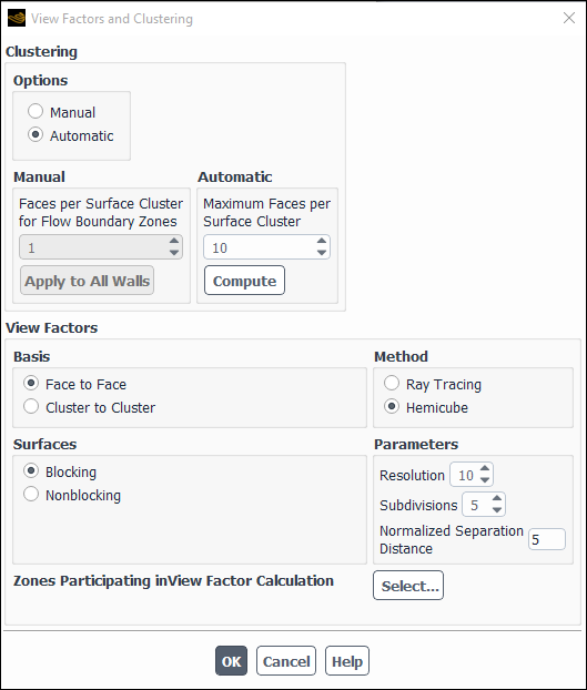
You can set the number of faces per surface cluster (FPSC) for each flow
boundary (that is, exhaust fan, inlet vent, intake fan, outlet vent,
mass-flow inlet, mass-flow outlet, pressure far-field, pressure inlet,
pressure outlet, outflow, and velocity inlet boundary) and wall that is
adjacent to a fluid zone; in this way, you can control the number of
radiating surfaces and (if you select Cluster to
Cluster for Basis) view factor surfaces.
By default, the FPSC value is set to  everywhere, so the number of surface clusters
(radiating/view factor surfaces) will be equal to the number of boundary
faces. For small 2D problems, this is an acceptable number. For larger
problems, you may want to reduce the number of surface clusters (that is,
increase the FPSC) to reduce both the size of the view factor file and the
memory requirement. Such a reduction in the number of clusters, however,
comes at the cost of some accuracy. Note that for a thermally coupled mesh
interface (that is, a fluid-fluid interface with Coupled
Wall enabled, or an interface involving a solid zone), the
FPSC is always set to 1. See Clustering in the Theory Guide for details about clustering.
everywhere, so the number of surface clusters
(radiating/view factor surfaces) will be equal to the number of boundary
faces. For small 2D problems, this is an acceptable number. For larger
problems, you may want to reduce the number of surface clusters (that is,
increase the FPSC) to reduce both the size of the view factor file and the
memory requirement. Such a reduction in the number of clusters, however,
comes at the cost of some accuracy. Note that for a thermally coupled mesh
interface (that is, a fluid-fluid interface with Coupled
Wall enabled, or an interface involving a solid zone), the
FPSC is always set to 1. See Clustering in the Theory Guide for details about clustering.
Important: If you plan to use the cluster to cluster basis for the view factor calculation, be sure that the FPSC values are appropriate for both the radiosity calculation and the view factors.
Note that during the creation of a cluster on a non-conformal interface, its parent thread is taken into the consideration; it may happen that the cluster is somewhat larger than its child face, which may lead some inaccuracy in the flux calculation.
The Clustering group box in the View Factors and Clustering dialog box (Figure 16.20: The View Factors and Clustering Dialog Box) provides two methods for revising the default FPSC values:
manual
automatic
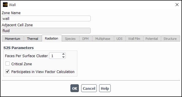
If you select Manual in the Options group box, you can specify an FPSC value for all flow boundaries in the Faces per Surface Cluster for Flow Boundary Zones number-entry box in the Manual group box. If you then click Apply to All Walls, you will apply this value to all wall zones that are adjacent to fluid zones as well. For a wall that requires a different FPSC value (that is, you may want a lower value for walls in critical areas, and higher values in non-critical areas), you will need to open the boundary condition dialog box (Figure 16.21: The Wall Dialog Box) for that particular wall and modify the Faces Per Surface Cluster in the S2S Parameters group box of the Radiation tab. Note that the Radiation tab also allows you to specify whether the wall participates in the view factor calculation, as described in Specifying Boundary Zone Participation.
Note:
Only zones attached to fluid cell zones are used for creating surface clusters.
Faces Per Surface Cluster (FPSC) is indicative of the actual reduction factor except when the surfaces are planar. The surface clustering algorithm uses other criteria (angle between faces, and so on) to ensure the clusters are nearly planar, so it is possible that there will be no further reduction in the total number of clusters beyond a certain value of FPSC.
Important: The Faces Per Surface Cluster number-entry box will not be visible in the GUI on wall boundary zones that are attached to a solid.
Using the manual method to specify the FPSC values for walls can become very cumbersome if the model involves a large number of radiating faces, which is typically the case in underhood models. In such circumstances, it is recommended that you use the automatic clustering method instead. In this method, different FPSC values are assigned to the walls automatically, based on the distance of the walls from and the FPSC values of the walls that are defined as critical. The steps you will need to take are as follows:
Select Automatic from the Options list in the View Factors and Clustering dialog box.
For each wall that you deem critical, perform the following actions in the Wall dialog box (Figure 16.21: The Wall Dialog Box):
Click the Radiation tab.
Enter an appropriate value for Faces Per Surface Cluster in the S2S Parameters group box.
Enable the Critical Zone option.
Click to close the Wall dialog box.
Enter the Maximum Faces per Surface Cluster value in the View Factors and Clustering dialog box and click the button. Ansys Fluent will automatically calculate and update the Faces Per Surface Cluster values for all Wall dialog boxes adjacent to fluid zones that do not have Critical Zone enabled, without computing the clusters.
You can check the automatically assigned FPSC values by opening the boundary condition dialog box of any non-critical wall of interest and examining the value for Faces Per Surface Cluster in the S2S Parameters group box of Radiation tab. You can manually modify the value for Faces Per Surface Cluster as necessary.
Whether you set the FPSC value manually or automatically, you have the
option of modifying the cutoff or “split” angle between
adjacent face normals for the purpose of controlling surface clustering.
The split angle sets the limit for which adjacent faces are clustered. A
smaller split angle allows for a better representation of the view
factor. By default, no surface cluster will contain any face that has a
face normal greater than 20°. To modify
the value of this parameter, you can use the
split-angle text command:
define →
models →
radiation →
s2s-parameters →
split-angle
You can control many aspects of how the view factors are calculated for your S2S model: how surfaces are defined; the computational method and related parameters; whether surface blocking will be accounted for; and which boundary zones will participate in the calculation. All of these controls are available in the View Factors group box in the View Factors and Clustering dialog box (Figure 16.20: The View Factors and Clustering Dialog Box), and are described in the sections that follow.
Ansys Fluent allows two ways to define the surfaces used for the view factor calculation, as described in Clustering and View Factors in the Theory Guide. If you want the surfaces to be the boundary faces of the mesh, select Face to Face for Basis in the View Factor group box of the View Factors and Clustering dialog box. This is the default selection.
Alternatively, you can select Cluster to Cluster for Basis, in order to reduce the computational expense and storage requirements. In this case, the surfaces used to calculate the view factors are the clusters defined by the settings in the Cluster group box of the View Factors and Clustering dialog box. The reduction in computational time will be proportional to the number of surface clusters used in the view factor calculation. The trade-offs of using the cluster to cluster basis for the calculation are that the accuracy may decrease, and the following limitations apply:
The mesh must be 3D.
You cannot subdivide the faces as part of the hemicube method parameters, which can cause the view factors to be overestimated.
Polyhedral meshes are restricted to 1 face per surface cluster.
When using Cluster to Cluster, surface clusters will form on non-conformal interfaces by default only with the Ray Tracing method enabled. If you do not want clusters to form on non-conformal interfaces, you can use the following command and answer
no.define/models/radiation/s2s-parameters/enable-mesh-interface-clustering?
Ansys Fluent provides two methods for computing view factors: the ray tracing method (which is selected by default) and the hemicube method. The following limitations apply:
The hemicube method is available only for 3D and axisymmetric cases.
The hemicube method should not be used when any of the zones are defined as periodic or symmetry boundaries, as these types are not currently supported.
For the ray tracing method, when running in distributed parallel mode (including with Microsoft Job Scheduler), the working directory must be shared across all machines.
The hemicube method uses a differential area-to-area method and calculates the view factors on a row-by-row basis. The view factors calculated from the differential areas are summed to provide the view factor for the whole surface. This method originated from the use of the radiosity approach in the field of computer graphics [33].
To use the hemicube method to compute the view factors, select Hemicube from the Method list in the View Factors and Clustering dialog box. It is recommended that you use the hemicube method for large, complex models with few obstructing surfaces between the radiating surfaces.
The hemicube method is based upon three assumptions about the geometry of the surfaces: aliasing, visibility, and proximity. To validate these assumptions, you can specify three different hemicube parameters, which can help you obtain better accuracy in calculating view factors. In most cases, however, the default settings will be sufficient.
Aliasing—The true projection of each visible face onto the hemicube can be accurately accounted for by using a finite-resolution hemicube. As described previously, the faces are projected onto a hemicube. Because of the finite resolution of the hemicube, the projected areas and resulting view factors may be overestimated or underestimated. Aliasing effects can be reduced by increasing the value of the Resolution of the hemicube in the Parameters group box.
Visibility—The visibility between any two faces does not change. In some cases, face
 has a complete view of face
  from its centroid, but some other face
 occludes much of face
  from face
  . In such a case, the hemicube method will
overestimate the view factor between face
. In such a case, the hemicube method will
overestimate the view factor between face  and face
  calculated from the centroid of face
 . This error can be reduced by subdividing face
 into smaller subfaces. You can specify the
number of subfaces by entering a value for
Subdivisions in the
Parameters group box. Note that you
cannot subdivide the faces when Cluster to
Cluster is selected for
Basis.
into smaller subfaces. You can specify the
number of subfaces by entering a value for
Subdivisions in the
Parameters group box. Note that you
cannot subdivide the faces when Cluster to
Cluster is selected for
Basis.Proximity—The distance between faces is great compared to the effective diameter of the faces. The proximity assumption is violated whenever faces are close together in comparison to their effective diameter or are adjacent to one another. In such cases, the distances between the centroid of one face and all points on the other face vary greatly. Since the view factor dependence on distance is nonlinear, the result is a poor estimate of the view factor.
In the Parameters group box, you can set a limit for the Normalized Separation Distance, which is the ratio of the minimum face separation to the effective diameter of the face. If the computed normalized separation distance is less than the specified value, the face will then be divided into a number of subfaces until the normalized distances of the subfaces are greater than the specified value. Alternatively, you can specify the number of subfaces to create for such faces by entering a value for Subdivisions.
While the hemicube method projects radiating surfaces onto a hemicube, the ray tracing method instead traces rays through the centers of every hemicube face to determine which surfaces are visible through that face. Note that the ray tracing method does not subdivide the faces (as can be done when using the hemicube method by setting the Subdivisions or Normalized Separation Distance parameters), and so the view factors may be less accurate than those calculated using the hemicube method for surfaces that have a normalized separation distance less than 5.
To use the ray tracing method to compute the view factors, select Ray Tracing from the Method list in the View Factors and Clustering dialog box. You can adjust the value of the Resolution in the Parameters group box in order to reduce the impact of aliasing effects, as described previously.
View factor calculations depend on the geometric orientations of surface pairs with respect to each other. Two situations may be encountered when examining surface pairs:
If there is no obstruction between the surface pairs under consideration, then they are referred to as “nonblocking” surfaces.
If there is another surface blocking the views between the surfaces under consideration, then they are referred to as “blocking” surfaces. Blocking will change the view factors between the surface pairs and require additional checks to compute the correct value of the view factors.
For cases with blocking surfaces, select Blocking from the Surfaces list in the View Factors and Clustering dialog box. For cases with nonblocking surfaces, you can choose either Blocking or Nonblocking without affecting the accuracy. However, it is better to choose Nonblocking for such cases, as it takes less time to compute.
You can choose to exclude walls and inlet and exit boundaries from participating in the view factor calculation. If you are unsure whether it is necessary to calculate view factors for a particular boundary zone ahead of time, it is recommended that you allow it to participate; you can always reverse this decision as part of a future calculation run.
There are two ways in which you can enable/disable the participation of walls and inlet and exit boundaries in the view factor calculation. One of those ways is to use the Participates in View Factor Calculation option in the Radiation tab of the boundary condition dialog box. The other method is to use the Participating Boundary Zones dialog box (Figure 16.22: The Participating Boundary Zones Dialog Box), which is accessed by clicking the button next to the Zones Participating in View Factor Calculation label in the View Factors and Clustering dialog box. For cases that are made up of a very large number of zones, such as underhood applications, the latter method is recommended.
Important: If you compute the view factors and then later alter which boundary zones participate in the view factor calculation, you must recompute the view factors so that the data is up to date.
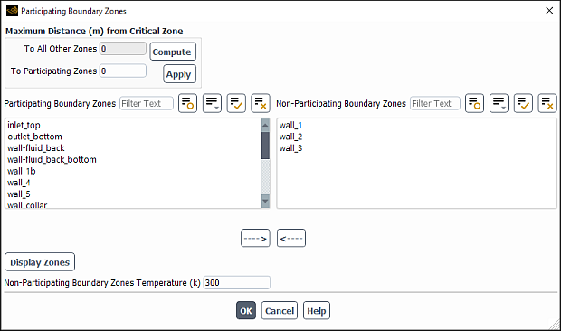
The Participating Boundary Zones dialog box allows you to easily specify those zones that are participating or non-participating without having to visit the boundary conditions dialog box of each zone. For cases that have a small number of boundary zones, you can simply select the zones that you do not want to participate in the view factor calculation from the Participating Boundary Zones list and click the arrow button that points to the right, so that the zones are moved to the Non-Participating Boundary Zones list; if you make an error, you can always reverse this process (that is, select a zone in the Non-Participating Boundary Zones list and click the arrow button that points to the left). This can be cumbersome for cases that have a large number of boundary zones, and so the following procedure is recommended instead:
Make sure that your clustering options (see Forming Surface Clusters) are appropriate for your view factor settings:
Select Automatic from the Options list in the Clustering group box of the View Factors and Clustering dialog box, as this enables some GUI items in the Participating Boundary Zones dialog box.
Important: Note that if you do not want to use the Automatic option for the clustering, you can revert to the Manual option after you are done using the Participating Boundary Zones dialog box.
Verify that the walls you specified as critical (by enabling the Critical Zone option in the Radiation tab of the boundary condition dialog box) also correspond to those that are critical for the view factor calculation. You must have specified at least one critical zone for the steps that follow.
Click the button in the Maximum Distance from Critical Zone dialog box, to update the value displayed for To All Other Zones. This value represents the maximum distance between the centroids of a critical zone and a non-critical zone in the mesh; it is for information purposes only, and cannot be edited in this dialog box.
Based on the value displayed for To All Other Zones, enter a threshold value for To Participating Zones. The value you enter will specify the maximum distance allowed between the centroids of a critical zone and a zone that participates in the view factor calculation. Then click the button to move all zones beyond this distance into the Non-Participating Boundary Zones list.
Review the zones displayed in the Participating Boundary Zones and Non-Participating Boundary Zones lists. If necessary, select zones in these lists and use the arrow buttons to move them to the appropriate list, as described previously.
If at any point you want to visually identify zones displayed in the Participating Boundary Zones and Non-Participating Boundary Zones lists, select the zones and click the button. Only the selected zones will be displayed in the graphics window.
If any zones are displayed in the Non-Participating Boundary Zones list, ensure to enter an appropriate temperature for Non-Participating Boundary Zones Temperature. In most cases the appropriate value is the ambient temperature, which by default is assumed to be 300 K.
After you have specified which zones do not participate in view factor calculation and set their temperature, click to store the settings and close the Participating Boundary Zones dialog box. You can then proceed to computing the view factors, as described in the section that follows.
Ansys Fluent can compute the view factors for your problem in the current session and save them to a file for use in the current session and future sessions.
Note: You can accelerate view factor calculations by using Ansys Fluent in parallel. For more information see Accelerating View Factor Calculations Using General Purpose Graphics Processing Units (GPGPUs).
To compute view factors in your current Ansys Fluent session, you must first set the parameters for the view factor calculation in the View Factors and Clustering dialog box (see View Factors and Clustering Settings for details) and click to save them. When you have set the view factor and surface cluster parameters, click the button in the View Factors and Clustering group box of the Radiation Model dialog box. A Select File dialog box will open, prompting you for the name of the file to which you would like to save the surface cluster information and view factors.
View factor files can be created in any of the following formats:
CFF S2S format (
filename.s2s.h5)Selecting CFF S2S Files for Files of type automatically adds the
s2s.h5extension.S2S compressed format (
filename.s2s.gz)Selecting S2S Files for Files of type allows you to add the
s2s.gzextension.S2S format (
filename.s2s)Selecting S2S Files for Files of type allows you to add the
s2sextension.
Important: Writing S2S files in .h5 format has the following
limitations.
Not supported when using GPU acceleration.
Not supported for mixed Windows/Linux mode.
Note that when using the TUI, you must directly specify the extension in the file name you provide.
The option to Write Binary Files is enabled by default, which reduces the time needed to write and read view factor files. When you click in the Select File dialog box, Ansys Fluent writes the surface cluster information to the file. Ansys Fluent uses the surface cluster information to compute the view factors, save the view factors to the same file, and then automatically read the view factors. The Ansys Fluent console will report the status of the view factor calculation. For example:
 Completed 25% calculation of view factors

 Completed 50% calculation of view factors

 Completed 75% calculation of view factors

 Completed 100 % calculation of view factors
Important:
You must recompute the view factors if you take any of following actions after the initial computation:
if you alter which boundary zones participate in the view factor calculation (either by using the Participating Boundary Zones dialog box, or by enabling / disabling the Participates in View Factor Calculation option in the Radiation tab of the boundary condition dialog box)
if you scale or unscale the mesh by using the Scale Mesh dialog box
The view factor file format for this version of Ansys Fluent is known as the compressed row format (CRF) and is a more efficient way of writing view factors than in versions that are prior to Fluent 6.4. In the CRF format, only nonzero view factors with their associated cluster IDs are stored to the file. This reduces the size of the
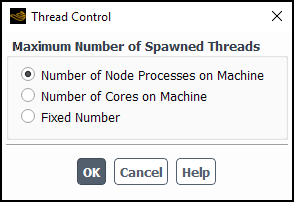
.s2sfile, and reduces the time it takes to read the file into Ansys Fluent. While the CRF file format is the default, you can still use the older file format if necessary. Contact your support engineer for more information.View factors using ray tracing are computed with the MPI/OpenMP hybrid model for parallel runs. By default, one OpenMP thread is used per MPI process, as specified in the Thread Control Dialog Box (see Controlling the Threads for details). To use all the available cores on your machine as OpenMP threads, select Number of Cores on Machine. A Fixed Number of cores can also be used based on your needs.
Note: For cases that use the S2S model and contain non-conformal interfaces, if the mesh interfaces are defined after the case has been read, then the intersection of the interface zones will occur during the initialization process, which will cause relabeling of faces throughout the domain. If you attempt to compute view factors before solution initialization in such a case, then the following message will be displayed in the console and the view factors will be computed automatically during solution initialization to avoid a mismatch with the case file:
Intersection zones for non-conformal interfaces are not created.
View factors will be computed during solution initialization.
If the view factors for your problem have already been computed and saved to a
file, you can read them into Ansys Fluent. To read in the view factors, click
button in the View
Factors and Clustering group box of the Radiation
Model dialog box. A Select File dialog box
will open where you can specify the name of the file containing the view
factors. For Files of type, select CFF S2S
Files to read .h5 files or select
S2S Files to read other formats. Alternatively, you can
read the view factors file using the File/Read/View
Factors... ribbon tab item.
For information about setting up the DO model, see the following sections:
For information about accelerating the DO solver, see Accelerating Discrete Ordinates (DO) Radiation Calculations.
When you select the Discrete Ordinates model, the Radiation Model dialog box will expand to show inputs for Angular Discretization (see Figure 16.16: The Radiation Model Dialog Box (DO Model)). In this section, you will set parameters for the angular discretization and pixelation described in Angular Discretization and Pixelation in the Theory Guide.
Theta Divisions ( ) and Phi Divisions (
 ) will define the number of control angles used to discretize
each octant of the angular space (see Figure 5.3: Angular Coordinate System in the Theory Guide). Note that higher levels of
discretization are recommended for problems where specular exchange of radiation
is important to increase the likelihood of the correct beam direction being
captured. For a 2D model, Ansys Fluent will solve only 4 octants (due to
symmetry); therefore, a total of
) will define the number of control angles used to discretize
each octant of the angular space (see Figure 5.3: Angular Coordinate System in the Theory Guide). Note that higher levels of
discretization are recommended for problems where specular exchange of radiation
is important to increase the likelihood of the correct beam direction being
captured. For a 2D model, Ansys Fluent will solve only 4 octants (due to
symmetry); therefore, a total of  directions
  will be solved. For a 3D model, 8 octants are solved,
resulting in
will be solved. For a 3D model, 8 octants are solved,
resulting in  directions
  . By default, the number of Theta
Divisions and the number of Phi Divisions
are both set to 2. For most practical problems, these settings are acceptable,
however, a setting of 2 is considered to be a coarse estimate. Increasing the
discretization of Theta Divisions and Phi
Divisions to a minimum of 3, or up to 5, will achieve more
reliable results. A finer angular discretization can be specified to better
resolve the influence of small geometric features or strong spatial variations
in temperature, but larger numbers of Theta Divisions and
Phi Divisions will add to the cost of the
computation.
. By default, the number of Theta
Divisions and the number of Phi Divisions
are both set to 2. For most practical problems, these settings are acceptable,
however, a setting of 2 is considered to be a coarse estimate. Increasing the
discretization of Theta Divisions and Phi
Divisions to a minimum of 3, or up to 5, will achieve more
reliable results. A finer angular discretization can be specified to better
resolve the influence of small geometric features or strong spatial variations
in temperature, but larger numbers of Theta Divisions and
Phi Divisions will add to the cost of the
computation.
Theta Pixels and Phi Pixels are used
to control the pixelation that accounts for any control volume overhang (see
Figure 5.7: Pixelation of Control Angle in the Theory Guide and the
figures and discussion preceding it). For problems involving gray-diffuse
radiation, the default pixelation of  is usually sufficient. For problems involving symmetry,
periodic, specular, or semi-transparent boundaries, a pixelation of
is usually sufficient. For problems involving symmetry,
periodic, specular, or semi-transparent boundaries, a pixelation of
 is recommended and will achieve acceptable results. The
computational effort, as a result of increasing the pixelation, is less than the
computational effort caused by increasing the divisions. You should be aware,
however, that increasing the pixelation adds to the cost of computation.
is recommended and will achieve acceptable results. The
computational effort, as a result of increasing the pixelation, is less than the
computational effort caused by increasing the divisions. You should be aware,
however, that increasing the pixelation adds to the cost of computation.
Important: Note that pixelations are applied to boundary faces by default.
If you want to model non-gray radiation using the DO model, you can specify
the Number of Bands ( ) under Non-Gray Model in the expanded
Radiation Model dialog box (Figure 16.24: The Radiation Model Dialog Box (Non-Gray DO Model)). For a 2D model, Ansys Fluent will
solve
) under Non-Gray Model in the expanded
Radiation Model dialog box (Figure 16.24: The Radiation Model Dialog Box (Non-Gray DO Model)). For a 2D model, Ansys Fluent will
solve  directions. For a 3D model,
  directions will be solved. By default, the Number of
Bands is set to zero, indicating that only gray radiation will be
modeled. Because the cost of computation increases directly with the number of
bands, you should try to minimize the number of bands used. In many cases, the
absorption coefficient or the wall emissivity is effectively constant for the
wavelengths of importance in the temperature range of the problem. For such
cases, the gray DO model can be used with little loss of accuracy. For other
cases, non-gray behavior is important, but relatively few bands are necessary.
For typical glasses, for example, two or three bands will frequently
suffice.
directions will be solved. By default, the Number of
Bands is set to zero, indicating that only gray radiation will be
modeled. Because the cost of computation increases directly with the number of
bands, you should try to minimize the number of bands used. In many cases, the
absorption coefficient or the wall emissivity is effectively constant for the
wavelengths of importance in the temperature range of the problem. For such
cases, the gray DO model can be used with little loss of accuracy. For other
cases, non-gray behavior is important, but relatively few bands are necessary.
For typical glasses, for example, two or three bands will frequently
suffice.
When a nonzero Number of Bands is specified, the
Radiation Model dialog box will expand once again to
show the Wavelength Intervals (Figure 16.24: The Radiation Model Dialog Box (Non-Gray DO Model)). You can specify a
Name for each wavelength band, as well as the
Start and End wavelength of the
band in  m. Note that the wavelength bands are specified for vacuum
(
m. Note that the wavelength bands are specified for vacuum
( ). Ansys Fluent will automatically account for the refractive
index in setting band limits for media with
). Ansys Fluent will automatically account for the refractive
index in setting band limits for media with  different from unity.
The frequency of radiation remains constant as radiation travels across a
semi-transparent interface. The wavelength, however, changes such that
 is constant. Therefore, when radiation passes from a medium
with refractive index
is constant. Therefore, when radiation passes from a medium
with refractive index  to one with refractive index
  , the following relationship holds:
 | (16–3) |
Here  and
and  are the wavelengths associated with the two media. It is
conventional to specify the wavelength rather than frequency.
Ansys Fluent requires you to specify wavelength bands (in
are the wavelengths associated with the two media. It is
conventional to specify the wavelength rather than frequency.
Ansys Fluent requires you to specify wavelength bands (in  m) for an equivalent medium with
  .
.
For example, consider a typical glass with a step jump in the absorption
coefficient at a cut-off wavelength of  . The absorption coefficient is
  for
for  and
and  for
for  . The refractive index of the glass is
  . Since
  is constant across a semi-transparent interface, the
equivalent cut-off wavelength for a medium with
is constant across a semi-transparent interface, the
equivalent cut-off wavelength for a medium with  is
is  using Equation 16–3. You should choose two
bands in this case, with the limits 0 to
using Equation 16–3. You should choose two
bands in this case, with the limits 0 to  and
and  to 100. Here, the upper wavelength limit has been chosen to be
a large number, 100, in order to ensure that the entire spectrum is covered by
the bands. When multiple materials exist, you should convert all the cut-off
wavelengths to equivalent cut-off wavelengths for an
to 100. Here, the upper wavelength limit has been chosen to be
a large number, 100, in order to ensure that the entire spectrum is covered by
the bands. When multiple materials exist, you should convert all the cut-off
wavelengths to equivalent cut-off wavelengths for an  medium, and choose the band boundaries accordingly.
The bands can have different widths and need not be contiguous. You can ensure
that the entire spectrum is covered by your bands by choosing  and
and  . Here
  and
and  are the minimum and maximum wavelength bounds of your
wavelength bands, and
are the minimum and maximum wavelength bounds of your
wavelength bands, and  is the minimum expected temperature in the domain.
Ansys Fluent allows you to use a user-defined function (UDF) to modify the
emissivity weighting factor  (which otherwise defaults to the black body emission factor
obtained from a standard Planck distribution). The emissivity weighting factor
appears in the emission term of the radiative transfer equation for the non-gray
model, as shown in Equation 5–100 in the Theory Guide. For more information, see
(which otherwise defaults to the black body emission factor
obtained from a standard Planck distribution). The emissivity weighting factor
appears in the emission term of the radiative transfer equation for the non-gray
model, as shown in Equation 5–100 in the Theory Guide. For more information, see DEFINE_EMISSIVITY_WEIGHTING_FACTOR in
the Fluent Customization Manual.
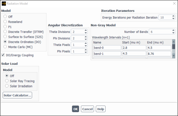
For applications involving optical thicknesses greater than 10, you can enable the DO/Energy Coupling option in the Radiation Model (Figure 16.25: The Radiation Model Dialog Box with DO/Energy Coupling Enabled) in order to couple the energy and intensity equations at each cell, solving them simultaneously. This approach accelerates the convergence of the finite volume scheme for radiative heat transfer and can be used with the gray or non-gray radiation model.
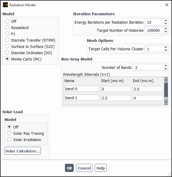
In the Iteration Parameters group box of the Radiation Model dialog box, you have the option of revising the Target Number of Histories to be tracked for the Monte Carlo (MC) simulation. The default value is 100,000. This can have a large effect on the accuracy of simulation results. For details, see Monte Carlo Solution Accuracy in the Theory Guide.
In some cases, Fluent might calculate substantially more histories than the specified Target Number of Histories, particularly if a fine surface mesh is used. The solver will ensure that an appropriate minimum number of histories are started at each surface face, and that can increase the total number of histories that are used during the calculation. Thus the CPU usage may not scale directly with changes to the specified target.
In the Mesh Options group box, you can coarsen the radiation mesh by specifying a Target Cells Per Volume Cluster greater than one. By default, it is set to one which implies no coarsening. Any value greater than one reduces the number of effective cells in the domain used by the MC radiation model. The coarsening is achieved by merging cells together and, therefore, does not affect the surface mesh resolution or alter the faces of any merged cells. The reduction in cells may speed up the radiation calculation and reduce peak memory usage, however, it may also have an impact on solution accuracy.
You have the option specifying multiple radiation bands using the Non-Gray Model group box. For each desired band, you must specify a start and end wavelength similar to Defining Non-Gray Radiation for the DO Model.
When you are using the P-1, DO, MC, or Rosseland radiation model in Ansys Fluent, you
should be sure to define both the absorption and scattering coefficients of the
fluid in the Create/Edit Materials dialog box. Note that you
can either enter a constant value for these parameters, or you can specify them
using a user-defined function (UDF). For more information, see DEFINE_PROPERTY UDFs in the Fluent Customization Manual.
![]() Setup →
Setup → ![]() Materials
Materials
If you are modeling semi-transparent media using the DO or MC model, you should also define the refractive index for the semi-transparent fluid or solid material. When using the Rosseland model, you can specify the refractive index only for the fluid material. When using the P-1 model, you should define the refractive index for the fluid material only. For the DTRM, you need to define only the absorption coefficient.
If your model includes gas phase species such as combustion products, absorption
and/or scattering in the gas may be significant. The scattering coefficient should
be increased from the default of zero if the fluid contains dispersed particles or
droplets that contribute to scattering. Note that when using the non-gray model, you
cannot specify a different scattering coefficient for each band. Alternatively, you
can specify the scattering coefficient as a user-defined function (UDF). For more
information, see DEFINE_PROPERTY UDFs in the Fluent Customization Manual.
Ansys Fluent allows you to enter a composition-dependent absorption coefficient for
 and
and  mixtures, using the WSGGM. The method for computing a variable
absorption coefficient is described in Radiation in Combusting Flows in the Theory Guide. Radiation Properties
provides a detailed description of the procedures used for specification of
radiation properties.
mixtures, using the WSGGM. The method for computing a variable
absorption coefficient is described in Radiation in Combusting Flows in the Theory Guide. Radiation Properties
provides a detailed description of the procedures used for specification of
radiation properties.
If you are using the non-gray P-1, DO, or MC model, you can specify a
different constant absorption coefficient for each of the bands used by the
gray-band model, as described in Radiation Properties. You
cannot, however, compute a composition-dependent absorption coefficient in each
band. If you use the WSGGM to compute a variable absorption coefficient, the
value will be the same for all bands. Alternatively, you can specify a
user-defined function (UDF) for the absorption coefficient. For more
information, see DEFINE_PROPERTY UDFs in the Fluent Customization Manual.
If you are using the non-gray P-1, DO, or MC model, you can specify a different constant refractive index for each of the bands used by the gray-band model, as described in Radiation Properties. You cannot, however, compute a composition-dependent refractive index in each band.
When you set up a problem that includes radiation, you will set additional boundary conditions at inlets, outlets, and walls. These inputs are described in the sections that follow. The boundary condition dialog boxes can be opened by right-clicking the boundary name in the tree (under Setup/Boundary Conditions) and clicking Edit... in the menu that opens; alternatively, you can open them from the Boundary Conditions task page:
![]() Setup →
Setup → ![]() Boundary
Conditions
Boundary
Conditions
The following topics are discussed:
- 16.3.8.1. Inlet and Outlet Boundary Conditions
- 16.3.8.2. Wall Boundary Conditions for the DTRM, P-1, S2S, and Rosseland Models
- 16.3.8.3. Wall Boundary Conditions for the DO Model
- 16.3.8.4. Wall Boundary Conditions for the MC Model
- 16.3.8.5. Solid Cell Zones Conditions for the DO or MC Models
- 16.3.8.6. Thermal Boundary Conditions
When radiation is active, you can define the emissivity at each inlet and
exit boundary when you are defining boundary conditions in the associated
inlet or exit boundary dialog box (for example, Pressure
Inlet dialog box, Velocity Inlet dialog
box, Pressure Outlet dialog box). Enter the appropriate
value for Internal Emissivity. The default value for
all boundary types is 1. Alternatively, you can specify a user-defined
function for emissivity. For more information, see DEFINE_PROFILE in the
Fluent Customization Manual.
For the non-gray P-1, DO, and MC models, the specified constant emissivity will be used for all wavelength bands.
Important: The Internal Emissivity boundary condition is not available with the Rosseland model.
Ansys Fluent includes an option that allows you to take into account the influence of the temperature of the gas and the walls beyond the inlet/exit boundaries, and specify different temperatures for radiation and convection at inlets and exits. This is useful when the temperature outside the inlet or exit differs considerably from the temperature in the enclosure. For example, if the temperature of the walls beyond the inlet is 2000 K and the temperature at the inlet is 1000 K, you can specify the outside wall temperature to be used for computing radiative heat flux, while the actual temperature at the inlet is used for calculating convective heat transfer. To do this, you would specify a radiation temperature of 2000 K as the black body temperature.
Although this option allows you to account for both cooler and hotter outside walls, you must use caution in the case of cooler walls, since the radiation from the immediate vicinity of the hotter inlet or outlet almost always dominates over the radiation from cooler outside walls. If, for example, the temperature of the outside walls is 250 K and the inlet temperature is 1500 K, it might be misleading to use 250 K for the radiation boundary temperature. This temperature might be expected to be somewhere between 250 K and 1500 K; in most cases it will be close to 1500 K. Its value depends on the geometry of the outside walls and the optical thickness of the gas in the vicinity of the inlet.
In the flow inlet or exit dialog box (for example, Pressure Inlet dialog box, Velocity Inlet dialog box), select Specified External Temperature in the External Black Body Temperature Method drop-down list, and then enter the value of the radiation boundary temperature as the Black Body Temperature.
Important:
If you want to use the same temperature for radiation and convection, retain the default selection of Boundary Temperature as the External Black Body Temperature Method.
The Black Body Temperature boundary condition is not available with the Rosseland model.
For the DO and MC models, you also have the option of specifying the BC Type with the following options:
The boundary behaves as described in Emissivity and Black Body Temperature above.
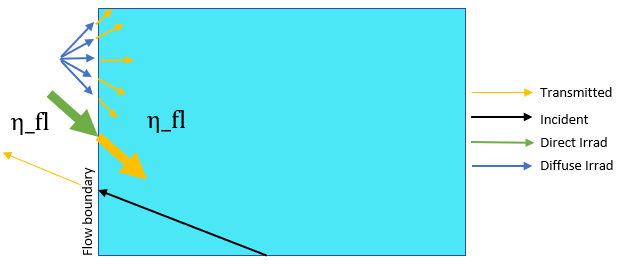
The boundary behaves similarly to an external semi-transparent wall, however, the irradiation flux passes through the transparent flow boundary from outside the computational domain into the adjacent fluid zone without getting reflected, absorbed or refracted (as shown in Figure 16.27: Treatment of Radiation at Transparent Boundary). For further details see, Semi-Transparent Exterior Walls in the Fluent Theory Guide.
The irradiation beam is defined in the same way as for an extremal semi-transparent wall. Specifically, for defining the beam width for the DO model, see Beam Width and Direction for External Irradiation Beam in the Fluent Theory Guide.
Incident radiation on a flow boundary from within the domain is also transmitted specularly.
Details for specifying a transparent boundary are similarly described for external semi-transparent wall boundaries for the DO and MC models, respectively.
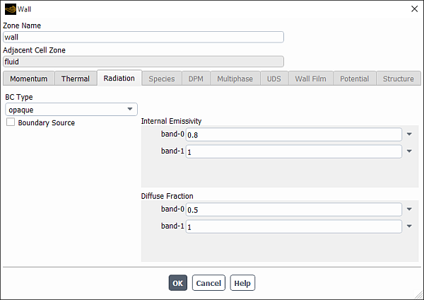
The DTRM, S2S, Rosseland, and gray P-1 models assume all walls to be gray and
diffuse. The only radiation boundary condition required in the
Wall dialog box is the Internal
Emissivity. For the Rosseland model, the internal emissivity is
automatically set to 1. For the DTRM, S2S, and gray P-1 models, you can enter
the appropriate value for Internal Emissivity in the
Radiation tab of the Wall dialog
box. The default value is 1. Alternatively, you can specify a user-defined
function for Internal Emissivity. For more information, see
DEFINE_PROFILE in the
Fluent Customization Manual.
For the non-gray P-1 model, specify a constant Internal Emissivity for each wavelength band in the Radiation tab of the Wall dialog box (the default value in each band is 1). Alternatively, you can specify the internal emissivity using a boundary condition parameter (see Creating a New Parameter). See Defining Boundary Conditions for Radiation for details.
When the S2S model is used, you can specify that some of the walls and inlet and exit boundaries are not participating in the view factor calculation. This capability allows you to save time computing the view factors and also reduce the memory required to store the view factor file during the Ansys Fluent calculation. See Specifying Boundary Zone Participation for details.
Important:
Whenever you revise which boundary zones participate in the calculation, you will need to recompute the view factors.
The Flux Reports dialog box will not show the exact balance of the Radiation Heat Transfer Rate because the radiative heat transfer to those boundaries that do not participate in the view factor calculation is not included.
When the DO model is used, you can model opaque walls, as discussed in Boundary and Cell Zone Condition Treatment at Opaque Walls in the Theory Guide, as well as semi-transparent walls (Cell Zone and Boundary Condition Treatment at Semi-Transparent Walls in the Theory Guide).
You can use a diffuse wall to model wall boundaries in many industrial applications since, for the most part, surface roughness makes the reflection of incident radiation diffuse. For highly polished surfaces, such as reflectors or mirrors, the specular boundary condition is appropriate. The semi-transparent boundary condition can be appropriate, for example, when modeling for glass panes in air.
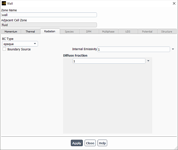
In the Radiation tab of the Wall dialog box (Figure 16.28: The Wall Dialog Box Showing Radiation Conditions for an Opaque Wall), select opaque in the BC Type drop-down list to specify an opaque wall.
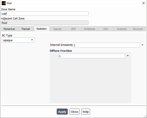
Specify the fraction of reflected radiation flux that is to be treated as
diffuse. By default, the Diffuse Fraction is set to
 , indicating that all of the radiation is diffuse. A
diffuse fraction equal to
, indicating that all of the radiation is diffuse. A
diffuse fraction equal to  indicates purely specular reflected radiation. A diffuse
fraction between
indicates purely specular reflected radiation. A diffuse
fraction between  and
and  will result in partially diffuse and partially specular
reflected energy. If the non-gray DO model is being used, the
Diffuse Fraction can be specified for each band.
See Boundary and Cell Zone Condition Treatment at Opaque Walls
in the Theory Guide for more details.
will result in partially diffuse and partially specular
reflected energy. If the non-gray DO model is being used, the
Diffuse Fraction can be specified for each band.
See Boundary and Cell Zone Condition Treatment at Opaque Walls
in the Theory Guide for more details.
For gray-radiation DO models, enter the appropriate value for Internal Emissivity (default value is 1). For non-gray DO models, specify a constant Internal Emissivity for each wavelength band in the Radiation tab of the Wall dialog box. (The default value in each band is 1.) Alternatively, you can specify the internal emissivity using a boundary condition parameter (see Creating a New Parameter).
You can also specify the external emissivity and external radiation
temperature for an opaque wall when the thermal conditions are set to
Radiation or Mixed in the
Wall dialog box (Figure 16.29: The Wall Dialog Box Showing External Emissivity and External
Radiation Temperature Thermal Conditions). Alternatively, you can
specify a UDF for these parameters; for more information, see DEFINE_PROFILE in the
Fluent Customization Manual.
Figure 16.29: The Wall Dialog Box Showing External Emissivity and External Radiation Temperature Thermal Conditions
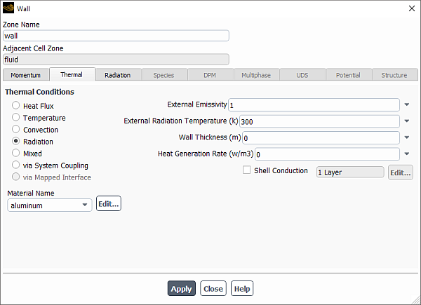
For more information on boundary condition treatment at opaque walls, see Boundary and Cell Zone Condition Treatment at Opaque Walls in the Theory Guide.
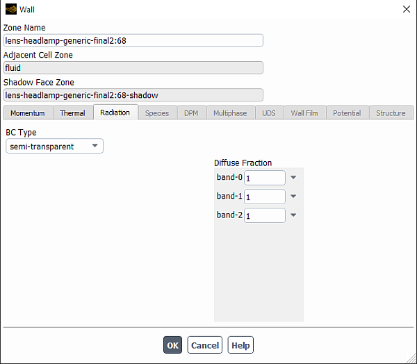
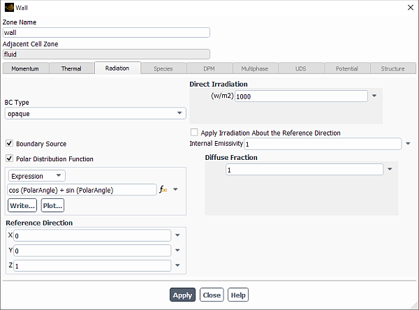
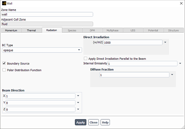
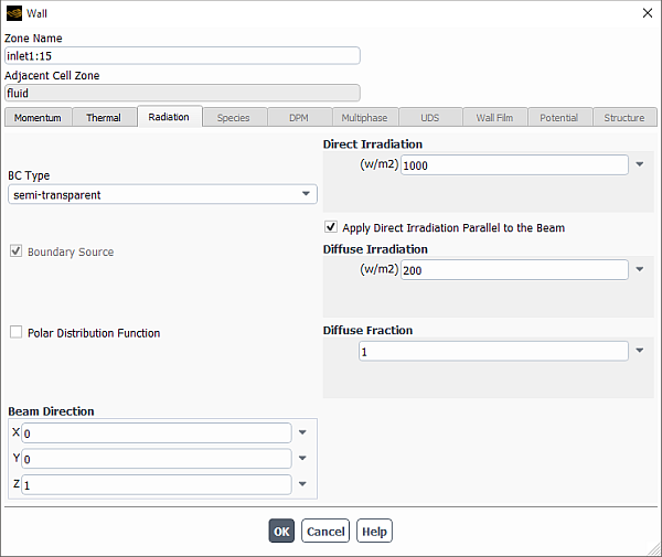
To define radiation for an exterior semi-transparent wall, click the Radiation tab in the Wall dialog box and then select semi-transparent in the BC Type drop-down list (Figure 16.30: The Wall Dialog Box for a Semi-Transparent Wall Boundary). The dialog box will expand to display the semi-transparent wall inputs needed to define an external irradiation flux (Figure 16.30: The Wall Dialog Box for a Semi-Transparent Wall Boundary).
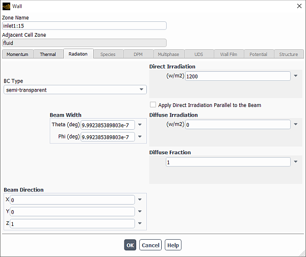
Then perform the following steps:
Specify the value of the irradiation flux (in W/m2) under Direct or Diffuse Irradiation. If the non-gray DO model is being used, a constant Direct or Diffuse Irradiation can be specified for each band.
Important: Note that the external diffuse irradiation specified when using Radiation or Mixed thermal conditions (selected in the Thermal tab), or Diffuse Irradiation (in the Radiation tab) is always distributed hemispherically after transmission through semi-transparent walls (that is independent of whether the external semi-transparent boundary wall is defined as a diffusely or specularly reflecting type).
By default, Apply Direct Irradiation Parallel to the Beam is selected, which means Fluent assumes that the value you specify for Direct Irradiation is the irradiation flux parallel to the Beam Direction. When deselected, Ansys Fluent assumes that the value you specify for Direct Irradiation is the irradiation flux normal to the boundary. See Figure 5.12: DO Irradiation on External Semi-Transparent Wall in Semi-Transparent Exterior Walls in the Theory Guide for details.
Define the Beam Width by specifying the beam Theta and Phi extents. Beam width is specified as the solid angle over which the irradiation is distributed. The default value for beam width is
 , which is suitable for collimated beam radiation.
A beam width less than this is likely to result in zero irradiation
flux.
, which is suitable for collimated beam radiation.
A beam width less than this is likely to result in zero irradiation
flux.Specify the (X,Y,Z) vector that defines the Beam Direction. The beam direction is defined as the vector of the centroid of the solid angle (beam width). You can specify the Beam Direction as a constant, a profile or a UDF. This is especially useful in applications where the shape of the radiative source is circular or cylindrical (or nonlinear). For information about boundary profiles, see Reading and Writing Profile Files.
Note that the actual direction of the beam of radiation that enters the domain will be further influenced by the solid angles available from the number of divisions set up; the effective direction will be the direction vector of the solid angle that the incoming beam falls into. Finally, any nonzero diffuse fraction will act to spread out (hemispherically, proportional to the diffuse fraction) the irradiation that enters the domain.
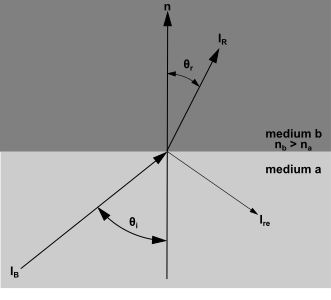
Note that the refractive index of the external medium is assumed to be 1. Therefore, if the refractive index of the fluid or solid material adjacent to the semi-transparent boundary is greater than 1, the direction of the prescribed direct irradiation after entering the computational domain will change due to refraction, and the magnitude of the incident radiation can be determined according to Figure 16.31: Refraction of Irradiation Entering Computational Domain.
For a UDF example that specifies the beam direction, see Example 5 - Beam Direction Profile at Semi-Transparent Walls in the Fluent Customization Manual.
Specify the Diffuse Fraction, the fraction of the reflected radiation from the wall that is treated as diffuse between 0 and 1. By default, the Diffuse Fraction is set to 1, indicating that all of the radiation is diffuse. A Diffuse Fraction of 0 treats the reflected radiation as purely specular. If you specify a value between 0 and 1, the radiation is treated as partially diffuse and partially specular. If the non-gray DO model is being used, the Diffuse Fraction can be specified for each band. See Diffuse Semi-Transparent Walls in the Theory Guide for details.
Important:
If Heat Flux conditions are specified in the Thermal tab of the Wall dialog box, the specified heat flux is considered to be only the conduction and convection portion of the boundary flux. The given irradiation specifies the incoming exterior radiative flux; the radiative flux transmitted from the domain interior to the outside is computed as a part of the calculation by Ansys Fluent. Internal emissivity is ignored for semi-transparent surfaces.
Note that when a boundary wall is made semi-transparent Ansys Fluent calculates the amount of radiation leaving as well as entering the domain. If you do not provide a source of irradiation or a radiating thermal condition (for example Mixed or Radiation) then you are effectively radiating to a temperature of
 K and it is highly likely you may observe
temperatures in your model that are lower than expected. Ensure
that the external (incoming) radiant conditions give good
account of the surroundings.
K and it is highly likely you may observe
temperatures in your model that are lower than expected. Ensure
that the external (incoming) radiant conditions give good
account of the surroundings.
You can also specify the external emissivity and external radiation
temperature for a semi-transparent wall when the thermal conditions are set
to Radiation or Mixed in the
Wall dialog box (Figure 16.29: The Wall Dialog Box Showing External Emissivity and External
Radiation Temperature Thermal Conditions). Alternatively, you can
specify a user-defined function (UDF) for these parameters; for more
information, see DEFINE_PROFILE in the Fluent Customization Manual.
Important: Note that for semi-transparent walls, Internal Emissivity is not available. If you want to include the effect of internal emissivity at semi-transparent walls, you must create a solid zone and specify that it participates in the radiation calculation; see Solid Semi-Transparent Media in the Theory Guide for details.
For a detailed description of boundary condition treatment at semi-transparent walls, see Cell Zone and Boundary Condition Treatment at Semi-Transparent Walls in the Theory Guide.
To define radiation for an interior (two-sided) semi-transparent wall, in the Wall dialog box, click the Radiation tab and then select semi-transparent in the BC Type drop-down list (Figure 16.32: The Wall Dialog Box for an Interior Semi-Transparent Wall). Then specify the Diffuse Fraction as described for the previous case.
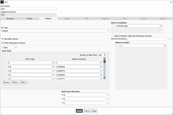
When the MC model is used, you can model walls as opaque or semi-transparent. Semi-transparent walls allows for the transmission of radiation through the wall (such as glass) whereas an opaque wall does not. Except in the case of an internal semi-transparent wall, you can also specify a Boundary Source where the wall will act as a radiation source with the specified characteristics (such as a light source).
In the Radiation tab of the Wall dialog box (Figure 16.33: The Wall Dialog Box for an Opaque Wall with MC Model (Gray)), select opaque in the BC Type.
You have the option of specifying an irradiation flux by selecting Boundary Source. (Figure 16.34: The Wall Dialog Box for an Opaque Wall with MC Model (Boundary Source))
Specify the value of the irradiation flux (in W/m2) under Direct Irradiation. If the non-gray MC model is being used, a constant Direct Irradiation can be specified for each band.
Specify the (X,Y,Z) vector that defines the Beam Direction. To model an isotropic source, you must set the Beam Direction to
0,0,0.Note: For multiband cases, if Direct Sources are zero for all bands, and you want to model a diffuse source, copy the band-wise diffuse sources to direct sources (band0 to band0, and so on). When doing this, specify the Directional Vector as zero (0,0,0). This will model the diffuse source per band as expected.
By default, Apply Direct Irradiation Parallel to the Beam is selected, which means Fluent assumes that the value you specify for Direct Irradiation is the irradiation flux parallel to the Beam Direction. When deselected, Ansys Fluent assumes that the value you specify for Direct Irradiation is the irradiation flux normal to the boundary.
Optionally select Polar Distribution Function, which can be used if the irradiation intensity varies with direction, but is rotationally symmetric about a given direction. For example, LED light sources.
You have the option of specifying a polar distribution via an Expression or Table.
If you select Expression (Figure 16.35: The Wall Dialog Box for an Opaque Wall with MC Model (Polar Distribution with Expression)), enter an expression to define the polar distribution as a function of "PolarAngle". For example:
cos(PolarAngle) + sin(PolarAngle)
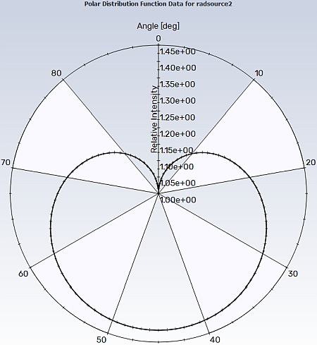
The expression is evaluated at 100 angles between 0 and 90 degrees to form data pairs of Polar Angle and Relative Intensity. You can write this polar distribution data via a
.csvfile using the Write... button or create a polar coordinates plot in the graphics window using the Plot... button (as shown in Figure 16.36: Polar Coordinate Plot of Radiation Intensity for Polar Distribution Function).Figure 16.35: The Wall Dialog Box for an Opaque Wall with MC Model (Polar Distribution with Expression)
If you select Table (Figure 16.37: The Wall Dialog Box for an Opaque Wall with MC Model (Polar Distribution with Table)), you must manually enter the data pairs or read a previously created
.csvfile.Select the Number of Data Pairs to define the polar coordinate system for your irradiation source.
Enter the data pairs in the form of Angle and Relative Intensity.
Note that the minimum number of data pairs is 2 and must include relative intensity data for 0 degrees. All angles must be between 0 and 90 degrees. Relative Intensity is typically between 0 and 1 although it does not have to be. A Relative Intensity of zero at a given angle means there is no radiation in that direction.
You have the option of reading and writing the polar distribution data (via
.csvfiles) using the Read... and Write... buttons. You can create a polar coordinate plot in the graphics window by selecting Plot... (as shown in Figure 16.36: Polar Coordinate Plot of Radiation Intensity for Polar Distribution Function).
Specify the (X,Y,Z) vector that defines the Reference Direction. This determines the center of the polar distribution function.
By default, Apply Irradiation About the Reference Direction is selected, which means Fluent assumes that the value you specify for Direct Irradiation is the irradiation flux parallel to the Reference Direction. When deselected, Ansys Fluent assumes that the value you specify for Direct Irradiation is the irradiation flux normal to the boundary.
You will also be required to specify the Internal Emissivity or, in the case of the non-gray MC model, specify an Internal Emissivity for each wavelength band.
You can also specify the external emissivity and external radiation temperature for an external wall when the thermal conditions are set to Radiation or Mixed in the Wall dialog box (Figure 16.39: The Wall Dialog Box Showing External Emissivity and External Radiation Temperature Thermal Conditions).
Figure 16.39: The Wall Dialog Box Showing External Emissivity and External Radiation Temperature Thermal Conditions
Specify the Diffuse Fraction, the fraction of the reflected radiation from the wall that is treated as diffuse between 0 and 1. By default, the Diffuse Fraction is set to 1, indicating that all of the radiation is diffuse. A diffuse fraction of 0 treats the radiation as purely specular. If you specify a value between 0 and 1, the radiation is treated as partially diffuse and partially specular. If the non-gray MC model is being used, the Diffuse Fraction can be specified for each band.
Note: For two-sided walls, while thermal boundary conditions are copied between a wall and it's shadow, any specified irradiation is not copied and each side of the wall is treated separately.
To define radiation for a semi-transparent wall, click the Radiation tab in the Wall dialog box and then select semi-transparent in the BC Type.
For internal semi-transparent walls, the boundary source option is not available. Specify the Internal Emissivity and Diffuse Fraction as described in Opaque Walls for the MC Model.
For external semi-transparent walls, Boundary Source is automatically enabled.
Provide the external irradiation as described in Opaque Walls for the MC Model, although you can specify Direct or Diffuse Irradiation for semi-transparent external walls when using the MC model as shown in Figure 16.40: The Wall Dialog Box for a Semi-transparent Wall with MC Model.
If you specify the external emissivity and external radiation temperature for a semi-transparent wall when the thermal conditions are set to Radiation or Mixed in the Wall dialog box, the external irradiation is treated as diffuse.
Important:
Note that the refractive index of the external medium is assumed to be 1.
If Heat Flux conditions are specified in the Thermal tab of the Wall dialog box, the specified heat flux is considered to be only the conduction and convection portion of the boundary flux. The given irradiation specifies the incoming exterior radiative flux; the radiative flux transmitted from the domain interior to the outside is computed as a part of the calculation by Ansys Fluent. Internal emissivity is ignored for semi-transparent surfaces.
Note that when a boundary wall is made semi-transparent Ansys Fluent calculates the amount of radiation leaving as well as entering the domain. If you do not provide a source of irradiation or a radiating thermal condition (for example Mixed or Radiation) then you are effectively radiating to a temperature of
K and it is highly likely you may observe
temperatures in your model that are lower than expected. Ensure
that the external (incoming) radiant conditions give good
account of the surroundings.Internal Emissivity is assumed to be zero for external semi-transparent walls. For Internal semi-transparent walls, internal emissivity is only required on walls between fluid and solid zones, or between two solid zones.
For a detailed description of boundary condition treatment at semi-transparent walls (for the DO model), see Cell Zone and Boundary Condition Treatment at Semi-Transparent Walls in the Theory Guide.
With the DO or MC model, you can specify whether or not you want to solve for radiation in each cell zone in the domain. By default, the DO or MC equations are solved in all fluid zones, but not in any solid zones. If you want to model semi-transparent media, for example, you can enable radiation in the solid zone(s). To do so, enable the Participates In Radiation option in the Solid dialog box (Figure 16.41: The Solid Dialog Box).
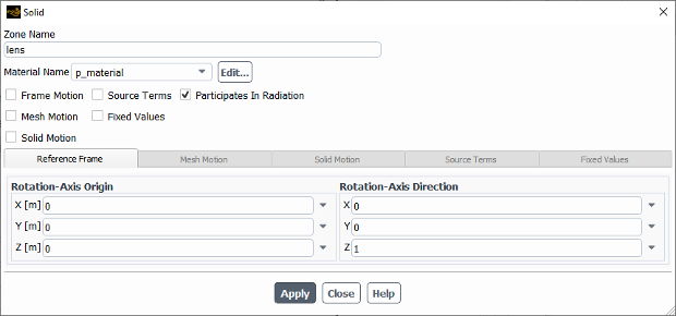
Important: In general, you should not disable the Participates In Radiation option for any fluid zones.
See Solid Semi-Transparent Media in the Theory Guide for more information on solid semi-transparent media.
In general, any well-posed combination of thermal boundary conditions can be used when any of the radiation models is active. The radiation model will be well-posed in combination with fixed temperature walls, conducting walls, and/or walls with set external heat transfer boundary conditions (Thermal Boundary Conditions at Walls). You can also use any of the radiation models with heat flux boundary conditions defined at walls, in which case the heat flux you define will be treated as the sum of the convective and radiative heat fluxes. The exception to this is the case of semi-transparent walls for the DO model. Here, Ansys Fluent allows you to specify the convective and radiative portions of the heat flux separately.
For the P-1, DTRM, S2S, DO, MC radiation models, there are several parameters that control the radiation calculation. You can use the default solution parameters for most problems, or you can modify these parameters to control the convergence and accuracy of the solution. Iteration parameters that are unique for a particular radiation model are specified in the Radiation Model dialog box. For the DTRM, S2S, DO, and MC models there are a common set of Iteration Parameters that control the frequency that the radiation model field is solved (as described in Iteration Parameters For Radiation Solve Frequency). Spatial Discretization (Discretization in the Theory Guide) and Under-Relaxation Factors (Under-Relaxation of Variables in the Theory Guide) are specified in the Solution Methods and Solution Controls task pages, respectively. The Convergence Criterion (Modifying Convergence Criteria) is set in the Residual Monitors dialog box.
There are no solution parameters to be set for the Rosseland model, since it impacts the solution only through the energy equation.
Important: If radiation is the only model being solved in Ansys Fluent and all other equations are disabled, then the radiation transfer equation will automatically be solved for every iteration.
For the P-1 radiation model, you can control the convergence criterion and under-relaxation factor. You should also pay attention to the optical thickness, as described below.
The default convergence criterion for the P-1 model is 10-6, the same as that for the energy equation, since the two are closely linked. See Monitoring Residuals for details about convergence criteria. You can set the Convergence Criterion for p1 in the Residual Monitors dialog box.
![]() Solution →
Monitors → Residuals
Solution →
Monitors → Residuals
![]() Edit...
Edit...
The under-relaxation factor for the P-1 model is set with those for other variables, as described in Setting Under-Relaxation Factors. Note that since the equation for the radiation temperature (Equation 5–60 in the Theory Guide) is a relatively stable scalar transport equation, in most cases you can safely use large values of under-relaxation (0.9–1.0).
For optimal convergence with the P-1 model, the optical thickness
 must be between 0.01 and 10 (preferably not larger than 5).
Smaller optical thicknesses are typical for very small enclosures
(characteristic size of the order of 1 cm), but for such problems you can
safely increase the absorption coefficient to a value for which
must be between 0.01 and 10 (preferably not larger than 5).
Smaller optical thicknesses are typical for very small enclosures
(characteristic size of the order of 1 cm), but for such problems you can
safely increase the absorption coefficient to a value for which  . Increasing the absorption coefficient will not change the
physics of the problem because the difference in the level of transparency of a
medium with optical thickness = 0.01 and one with optical thickness <0.01 is
indistinguishable within the accuracy level of the computation.
. Increasing the absorption coefficient will not change the
physics of the problem because the difference in the level of transparency of a
medium with optical thickness = 0.01 and one with optical thickness <0.01 is
indistinguishable within the accuracy level of the computation.
You can control the frequency that the radiation field is updated as the continuous phase solution proceeds for steady and transient simulations. For details, see Iteration Parameters For Radiation Solve Frequency.
When the DTRM is active, Ansys Fluent updates the radiation field during the calculation and computes the resulting energy sources and heat fluxes via the ray-tracing technique described in Ray Tracing in the Theory Guide. Ansys Fluent provides several solution parameters in the expanded portion of the Radiation Model dialog box (Figure 16.42: The Radiation Model Dialog Box (DTRM)).
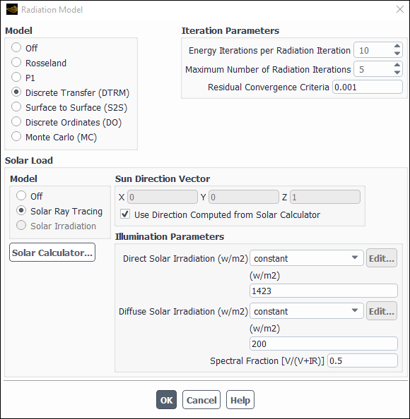
You can control the maximum number of iterations of the radiation calculation during each global iteration by changing the Maximum Number of Radiation Iterations. The default setting of 5 means that the radiosity will be updated up to 5 times. The actual number of iterations will be less if the residual convergence criterion is exceeded at any point during these iterations.
The Residual Convergence Criteria parameter (0.001 by default) determines when the radiation intensity update is converged. It is defined as the maximum normalized change in the surface intensity from one DTRM radiation iteration to the next (see Equation 16–4).
You can control the frequency that the radiation field is updated as the continuous phase solution proceeds for steady and transient simulations. For details, see Iteration Parameters For Radiation Solve Frequency.
You can control the maximum number of iterations of the radiation calculation during each global iteration by changing the Maximum Number of Radiation Iterations. The default setting of 5 means that the radiosity will be updated up to 5 times. The actual number of iterations will be less if the residual convergence criterion is exceeded at any point during these iterations.
The Residual Convergence Criteria (0.001 by default) determines when the radiosity update is converged. It is defined as the maximum normalized change in the radiosity from one S2S radiation iteration to the next (see Equation 16–5).
You can control the frequency that the radiation field is updated as the continuous phase solution proceeds for steady and transient simulations. For details, see Iteration Parameters For Radiation Solve Frequency.
For most problems, the default under-relaxation of 1.0 for the DO equations is
adequate. For problems with large optical thicknesses ( ), you may experience slow convergence or solution oscillation.
For such cases, under-relaxing the energy and DO equations is useful.
Under-relaxation factors between 0.9 and 1.0 are recommended for both
equations.
), you may experience slow convergence or solution oscillation.
For such cases, under-relaxing the energy and DO equations is useful.
Under-relaxation factors between 0.9 and 1.0 are recommended for both
equations.
You can control the frequency that the radiation field is updated as the continuous phase solution proceeds for steady and transient simulations. For details, see Iteration Parameters For Radiation Solve Frequency.
Wall Irradiation Flux.Normalized Std Deviation and
Radiation Intensity.Normalized Std Deviation (both
available during postprocessing) can give an indication of the quality of the
solution. They arise from the stochastic nature of the Monte Carlo model.
The Monte Carlo radiation solver computes the standard deviation error based on Poisson statistics. The user-specified number of histories is divided into several groups. Histories are selected from each group and their physical interactions (emission, absorption, reflection, and so on) are tracked through the domain. At the end of the calculation, each group provides values for the quantities of interest, such as irradiation heat flux or absorbed radiation. The mean value, and standard deviation, of each quantity of interest are computed from the groups. A normalized standard deviation is computed by dividing the standard deviation by the mean value.
Wall Irradiation Flux.Normalized Std Deviationis the maximum normalized standard deviation of the irradiation flux at an element face on a boundary. The presence of small isolated boundary regions with values ofWall Irradiation Flux.Normalized Std Deviationlarger than 30% is an indication that the element faces in those regions were insufficiently sampled. Increasing the Target Number of Histories may help address this, at the expense of computational effort.Radiation Intensity.Normalized Std Deviationis the maximum normalized standard deviation of the radiation intensity within an element. The value ofRadiation Intensity.Normalized Std Deviationis expected to be less than 30% within a reliable radiation field solution.
Because of the stochastic behavior, it can be difficult to judge the convergence of MC radiation cases based on residuals alone, particularly if the standard deviations are large. It is recommended that you create a temperature probe (for example, a Surface Report Definition) and monitor its stability during the solution. For more information, see Creating Report Definitions.
For the DTRM, S2S, DO, and MC models, you can control the frequency that the radiation field is updated as the continuous phase solution proceeds. The options available to control the radiation solve frequency depends on whether the simulation is steady or transient.
Steady Simulations
Under Iteration Parameters, the option Update
Radiation Based On can only be set to
iteration with the default Iteration
Interval set to 10. This means that the radiation calculation is
performed once every 10 iterations of the solution process. Increasing the
number can speed the calculation process, but may slow overall
convergence.
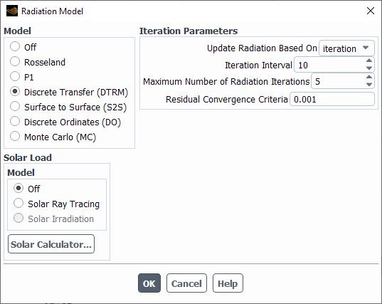
Note: If you are using the pressure-based solver with the S2S model and you first solve the flow equations with the energy equation turned off, you should reduce the Iteration Interval from 10 to 1 or 2. This will ensure the convergence of the radiosity. If the default value of 10 is kept in this case, it is possible that the flow and energy residuals may converge and the solution will terminate before the radiosity is converged.
Transient Simulations
Under Iteration Parameters, the option Update
Radiation Based On can be set to
time-step or
flow-time.
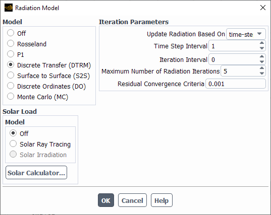
For updating radiation based on time-step, you must
specify the Time Step Interval and Iteration
Interval. The default value of 1 for Time Step
Interval means the radiation field will be updated every time
step. The default Iteration Interval of 0 means the
radiation field is updated after the first iteration in a time step. For
example, a Time Step Interval of 2 means the radiation
field is updated every other time step. An Iteration
Interval of 5 means the radiation field is updated every 5
iterations within a timestep.
For updating radiation based on flow-time, you must
specify the Time Interval in seconds and
Iteration Interval. The default value of 1 second for
Time Interval means the radiation field will be updated
once for every 1 second of flow time. The default Iteration
Interval of 0 means the radiation field is only updated to
satisfy the Time Interval condition. For example, a
Time Interval of 2 seconds means the radiation field is
updated after every 2 seconds of flow time. An Iteration
Interval of 5 means the radiation field is updated every 5
iterations within a timestep.
Once the radiation problem has been set up, you can proceed as usual with the calculation. Note that while the P-1 and DO models will solve additional transport equations and report residuals, the DTRM and the Rosseland and S2S models will not (since they impact the solution only through the energy equation). Residuals for the DTRM and S2S model radiation iterations are reported by Ansys Fluent every time such an iteration is performed, as described below.
When running the S2S model with the parallel solver, note that coupled walls are encapsulated, which may cause problems with the partitioning of the mesh. See Troubleshooting for recommendations on correcting such problems.
The residual for radiation as calculated by the P-1 model is updated after each iteration and reported with the residuals for all other variables. Ansys Fluent reports the normalized P-1 radiation residual as defined in Monitoring Residuals for the other transport equations.
After each DO iteration, the DO model reports a composite normalized residual for all the DO transport equations. The definition of the residuals is similar to that for the other transport equations (see Monitoring Residuals).
Ansys Fluent does not include a DTRM residual in its usual residual report that is issued after each iteration. The effect of radiation on the solution can be gathered, instead, via its impact on the energy field and the energy residual. However, each time a DTRM iteration is performed, Ansys Fluent will print out the normalized radiation error for each DTRM radiation iteration. The normalized radiation error is defined as
 | (16–4) |
where the error  is the maximum change in the intensity (
 ) at the current radiation iteration, normalized by the
maximum surface emissive power, and
) at the current radiation iteration, normalized by the
maximum surface emissive power, and  is the total number of radiating surfaces. Note that the
default radiation convergence criterion, as noted in DTRM Solution Parameters, defines the radiation calculation
to be converged when
is the total number of radiating surfaces. Note that the
default radiation convergence criterion, as noted in DTRM Solution Parameters, defines the radiation calculation
to be converged when  decreases to
  or less.
Ansys Fluent does not include an S2S residual in its usual residual report that is issued after each iteration. The effect of radiation on the solution can be gathered, instead, via its impact on the energy field and the energy residual. However, each time an S2S iteration is performed, Ansys Fluent will print out the normalized radiation error for each S2S radiation iteration. The normalized radiation error is defined as
 | (16–5) |
where the error  is the maximum change in the radiosity (
 ) at the current radiation iteration, normalized by the
maximum surface emissive power, and
) at the current radiation iteration, normalized by the
maximum surface emissive power, and  is the total number of radiating surface clusters. Note
that the default radiation convergence criterion, as noted in DTRM Solution Parameters, defines the radiation calculation
to be converged when
is the total number of radiating surface clusters. Note
that the default radiation convergence criterion, as noted in DTRM Solution Parameters, defines the radiation calculation
to be converged when  decreases to
  or less.
Sometimes, you may want to set up your Ansys Fluent model with the radiation model active and then disable the radiation calculation during the initial calculation phase. For the P-1 and DO models, you can turn off the radiation calculation temporarily by deselecting P1 or Discrete Ordinates in the Equations dialog box, which is accessed by right-clicking Solution Controls in the tree (under Solution) and clicking Equations... in the menu that opens. For the DTRM and the S2S model, there is no radiation calculation to disable in the Equations dialog box. You can instead set a very large number for Energy Iterations per Radiation Iteration in the Iteration Parameters group box of the Radiation Model dialog box.
If you turn off the radiation calculation, Ansys Fluent will skip the update of the radiation field during subsequent iterations, but will leave in place the influence of the current radiation field on energy sources due to absorption, wall heat fluxes, and so on. Turning the radiation calculation off in this way can therefore be used to initiate your modeling work with the radiation model inactive and/or to focus the computational effort on the other equations if the radiation model is relatively well converged.
Information regarding postprocessing radiation quantities can be found in the following sections:
Ansys Fluent provides radiation quantities that you can use in postprocessing when your model includes the solution of radiative heat transfer. You can generate graphical plots or alphanumeric reports of the following variables/functions:
In the Radiation... category:
Incident Radiation (P-1, DO, MC)
Incident Radiation (Band n) (non-gray P-1, non-gray DO, non-gray MC)
Absorption Coefficient (DTRM, P-1, DO, Rosseland)
Scattering Coefficient (P-1, DO, Rosseland)
Refractive Index (P1, DO, Rosseland)
Radiation Temperature (P-1, DO, MC)
Surface Cluster ID (S2S)
Volumetric Absorbed Radiation (P-1, DO, MC)
Volumetric Emitted Radiation (P-1, DO, MC)
Radiation Intensity.Normalized Std Deviation (MC)
Wall Irradiation Flux.Normalized Std Deviation (MC)
In the Wall Fluxes... category:
Radiation Heat Flux (All)
Surface Incident Radiation (S2S, DTRM, DO, MC)
Absorbed Radiation Flux (DO, MC)
Reflected Radiation Flux (DO, MC)
Transmitted Radiation Flux (DO, MC)
Beam Irradiation Flux (DO, MC)
See Field Function Definitions for definitions of these postprocessing variables. Note that in addition, incident radiation, transmitted, reflected and absorbed radiation flux are also available on a per-band basis for the non-gray DO model.
Important:
The sign convention on the radiative heat flux is such that the heat flux from the wall surface is a positive quantity.
It is possible to export heat flux data on wall zones (including radiation) to a generic file that you can examine or use in an external program. See Exporting Heat Flux Data for details.
Take care not to confuse Incident Radiation and Surface Incident Radiation. Incident Radiation is a volumetric quantity giving the total radiant load passing through the cell (in all directions), whereas Surface Incident Radiation is the total radiant load hitting the surface (which will subsequently be absorbed, transmitted and reflected). There is no direct means to report how much radiation has been absorbed/emitted/scattered in cells.
You can use the Flux Reports dialog box to compute the radiative heat transfer through each boundary of the domain, or to sum the radiative heat transfer through all boundaries.
![]() Results → Reports
→ Fluxes
Results → Reports
→ Fluxes
![]() Edit...
Edit...
See Fluxes Through Boundaries for details about generating flux reports.
The DTRM yields a global heat balance and a balance of radiant heat fluxes only in the limit of a sufficient number of rays. In any given calculation, therefore, if the number of rays is insufficient you may find that the radiant fluxes do not obey a strict balance. Such imbalances are the inevitable consequence of the discrete ray tracing procedure and can be minimized by selecting a larger number of rays from each wall boundary.
When you use the DTRM, Ansys Fluent allows you to display surface or volume clusters, as well as the rays that emanate from a particular surface cluster. You can use the DTRM Graphics dialog box (Figure 16.45: The DTRM Graphics Dialog Box) for all of these displays.
![]() Results → Model
Specific → DTRM Graphics...
Results → Model
Specific → DTRM Graphics...
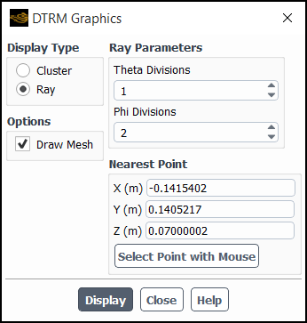
To view clusters, select Cluster under Display Type and then select either Surface or Volume under Cluster Type.
To display all of the surface or volume clusters, select the Display All Clusters option under Cluster Selection and click the button.
To display only the cluster (surface or volume) nearest to a specified point, deselect the Display All Clusters option and specify the coordinates under Nearest Point. You may also use the mouse to choose the nearest point. Click the button and then right-click a point in the graphics window.
To display the rays emanating from the surface cluster nearest to the specified point, select Ray under Display Type. Set the appropriate values for Theta and Phi Divisions under Ray Parameters (see Setting Up the DTRM for details), and then click the button. Figure 16.46: Ray Display shows a ray plot for a simple 2D geometry.
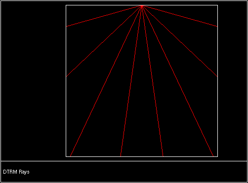
For some problems, especially complex 3D geometries, you may want to include portions of the mesh in your ray or cluster display as spatial reference points. For example, you may want to show the location of an inlet and an outlet along with displaying the rays. This is accomplished by enabling the Draw Mesh option in the DTRM Graphics dialog box. The Mesh Display dialog box will appear automatically when you enable the Draw Mesh option, and you can set the mesh display parameters there. When you click Display in the DTRM Graphics dialog box, the mesh display, as defined in the Mesh Display dialog box, will be included in the ray or cluster display.
When you use the S2S model, Ansys Fluent allows you to view the values of the view factor and radiation emitted from one zone to any other zone. You can use the S2S Information dialog box (Figure 16.47: The S2S Information Dialog Box) to generate a report of these values in the console or as a separate file.
![]() Results → Model
Specific → S2S Information...
Results → Model
Specific → S2S Information...
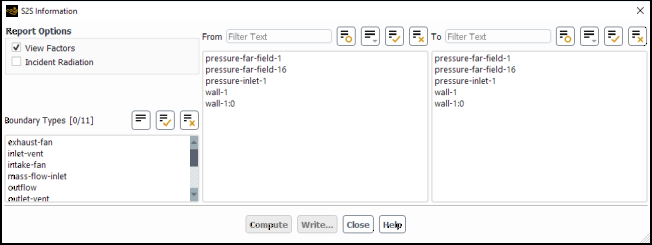
The steps for generating the report are as follows:
Specify the values in which you are interested by selecting View Factors and/or Incident Radiation.
Choose the zones for which you would like data by selecting them in the lists under From and To (at least one zone must be selected under each list). To select all of the zones of a particular type, click that category in the list under Boundary Types.
Specify how you would like to present the data. To report the values in the console, click the button. To write the data as an S2S Info File (
.sifformat), click the button and enter a file name in The Select File Dialog Box.
The following is an example of how the data is presented:
S2S Information
From wall1 to:
                    View factor       Incident Radiation
          wall1          0.0000                   0.0000
          wall2          0.2929              171387.7813
          wall3          0.2929              155305.7969
          wall4          0.4142               29055.9023

From wall2 to:
                    View factor       Incident Radiation
          wall1          0.2929              306451.9688
          wall2          0.0000                   0.0000
          wall3          0.4142              214195.0938
          wall4          0.2929               19153.2715
Note that the header listed above (S2S Information)
is not displayed in the console.
Ansys Fluent provides a solar load model that can be used to calculate radiation effects from the sun’s rays that enter a computational domain. Two options are available for the model: Solar Ray Tracing and Solar Irradiation. The Solar Ray Tracing approach is a highly efficient and practical means of applying solar loads as heat sources in the energy equations. In cases where you want to use the DO or MC model to calculate radiation effects within the domain, the Solar Irradiation option is available to supply outside beam direction and intensity parameters directly to the radiation model. The solar load model includes a solar calculator utility that can be used to construct the sun’s location in the sky for a given time-of-day, date, and position. Solar load is available in the 3D solver only, and can be used to model steady and unsteady flows.
Typical applications that are well-suited for solar load simulations include the following:
automotive climate control (ACC) applications
human comfort modeling applications in buildings
The effects of solar loading are needed in many ACC applications, where the temperature, humidity, and velocity fields around passengers (and drivers) are desired. ACC systems are tested for their capacity to cool down passenger compartments after they have been “soaked” in intense solar radiation. Ansys Fluent’s solar load model will enable you to simulate solar loading effects and predict the time it will take to reasonably cool down the cabin of a car that has been exposed to solar radiation, as well as predict the time interval needed to lower the temperature in specified points and areas within the domain.
In the analysis of buildings, solar loading provides a significant burden on the cooling requirement in warm climates, particularly where architects want to use the aesthetics of glazed facades. Even in cooler climates, solar loading can provide a burden during warmer seasons where modern buildings are well insulated against thermal loss during winter months. As well as providing an engineer with a practical tool for determining the solar heating effect inside a building, Ansys Fluent’s solar load model will allow the solar transmission through all glazed surfaces to be determined over the course of a day, allowing important decisions to be made before undertaking any flow studies. Ansys Fluent’s solar load model also allows you to simulate porous blinds, which can transmit a portion of the solar radiation while also allowing fluid flow.
The solar load model’s ray tracing algorithm can be used to predict the direct illumination energy source that results from incident solar radiation. It takes a beam that is modeled using the sun position vector and illumination parameters, applies it to any or all wall, porous jump, and inlet/outlet boundary zones that you specify, performs a face-by-face shading analysis to determine well-defined shadows on all boundary faces and interior walls, and computes the heat flux on the boundary faces that results from the incident radiation.
Important: The solar ray tracing model includes only boundary zones that are adjacent to fluid zones in the ray tracing calculation. Therefore, boundary zones that are attached to solid zones are treated as transparent and are not included in the ray tracing algorithm.
The resulting heat flux that is computed by the solar ray tracing algorithm is coupled to the Ansys Fluent calculation via a source term in the energy equation. The heat sources are added directly to computational cells bordering each face and are assigned to adjacent cells in the following order: shell conduction cells, solid cells, and fluid cells. Heat sources are assigned to one of these types of adjacent cells, only. You can choose to override this order and include adjacent fluid cells in the solar load calculation by issuing a command in the text user interface (see Text Interface-Only Commands for details). Note that the sun position vector and solar intensity can be entered either directly by you or computed from the solar calculator. Direct and diffuse irradiation parameters can also be specified using a user-defined function (UDF) and hooked to Ansys Fluent in the Radiation Model dialog box.
The solar ray tracing option allows you to include the effects of direct solar illumination as well as diffuse solar radiation in your Ansys Fluent model. A two-band spectral model is used for direct solar illumination and accounts for separate material properties in the visible and infrared bands. A single-band hemispherical-averaged spectral model is used for diffuse radiation. Opaque materials are characterized in terms of two-band absorptivities. A semi-transparent material requires specification of absorptivity and transmissivity. Values that you specify for transmissivity and absorptivity are defined for normal incident rays. Ansys Fluent recomputes/interpolates these values for the given angle of incidence.
The solar ray tracing algorithm also accounts for internal scattered and
diffusive loading. The reflected component of direct solar irradiation is
tracked. A fraction of this radiative heat flux, called internally scattered
energy is applied to all the surfaces participating in the solar load
calculation, weighted by area. The internally scattered energy depends on the
scattering fraction that is specified in the TUI, whose default value is
 . Depending on the reflectivity of the primary surface, the
scattering fraction can be responsible for the inclusion (or exclusion) of a
large amount of radiation within the rest of the domain.
. Depending on the reflectivity of the primary surface, the
scattering fraction can be responsible for the inclusion (or exclusion) of a
large amount of radiation within the rest of the domain.
Also included as internally scattered energy is the contribution of the transmitted component of diffuse solar irradiation (which enters a domain through semi-transparent walls depending upon the hemispherical transmissivity). The total value of internally scattered energy is reported to the Ansys Fluent console. The ambient flux is obtained by dividing the internally scattered energy by the total surface area of the faces participating in the solar load calculation.
Note that Solar Ray Tracing is not a participating radiation model. It does not deal with emission from surfaces, and the reflecting component of the primary incident load is distributed uniformly across all surfaces rather than being local to the surfaces reflected to. If surface emission is an important factor in your case then you can consider implementing a radiation model (for example, P-1) in conjunction with Solar Ray Tracing.
Note the following limitation when using the solar ray tracing model:
Non-conformal interfaces are not supported with Solar Ray Tracing.
If solving in parallel, Fluent computes Solar Ray Tracing on only the host process although the calculation does employ multiple threads. Therefore, it is important to ensure the host process has sufficient available RAM for the computation.
The shading calculation that is used for solar ray tracing is a straightforward application of vector geometry. A ray is traced from the centroid of a test face in the direction of the sun. Every other face is checked to determine if the ray intersects the candidate face and if the candidate face is in front of the test face. If both conditions are met, then an opaque face completely shades the test face. A semi-transparent face attenuates the incident energy.
A Barycentric coordinate formulation is used to construct triangle-ray
intersections. A quadrilateral ray intersection method is used to handle the
case when model surfaces contain quadrilaterals. A quad-tree preprocessing
step is applied to reduce the ray tracing algorithm complexity that can lead
to long run times for  faces and greater. The quad-tree refinement factor can be
modified in the text interface. The default value of this parameter is
faces and greater. The quad-tree refinement factor can be
modified in the text interface. The default value of this parameter is
 , which is sufficient to cover the entire spectrum of mesh
sizes between one cell and five million cells. If the mesh is greater than
five million cells, an increase in this parameter would reduce the CPU time
needed to compute the solar loads.
, which is sufficient to cover the entire spectrum of mesh
sizes between one cell and five million cells. If the mesh is greater than
five million cells, an increase in this parameter would reduce the CPU time
needed to compute the solar loads.
Incident solar radiation can be applied to glass and plastic glazing materials of various types at wall boundaries, and the effects of coated glazings modeled using the solar ray tracing algorithm. To model solar optical properties, you will need to specify the transmissivity and reflectivity of the material in the Wall boundary conditions dialog box. You can obtain these values from the glass (or plastic) manufacturer or use data from another source (for example, ASHRAE Handbook).
Glazing optical properties are dependent on incident angle, and the
variation is significant for an incident angle greater than  degrees. As the incident angle increases from zero,
transmissivity decreases, reflectivity increases, and absorptivity increases
initially due to lengthened optical path, and then decreases as more
incident radiation is reflected. The shape of the property curve varies with
glass type and thickness. This difference is more pronounced for coated
glass or for a multiple-pane glazing system. It cannot be assumed that all
glazing systems have a universal angular dependence.
degrees. As the incident angle increases from zero,
transmissivity decreases, reflectivity increases, and absorptivity increases
initially due to lengthened optical path, and then decreases as more
incident radiation is reflected. The shape of the property curve varies with
glass type and thickness. This difference is more pronounced for coated
glass or for a multiple-pane glazing system. It cannot be assumed that all
glazing systems have a universal angular dependence.
For coated glazings, the spectral transmissivity and reflectivity at any incident angle are approximated in the solar load model from the normal angle of incidence [45].
Transmissivity is given by
(16–6) |
where
 | (16–7) |
Reflectivity is given by
 | (16–8) |
where
 | (16–9) |
The constants used in Equation 16–6 and
Equation 16–8 are for coated glazings
and are taken from Finlayson and Arasteh. [45]. The normal transmissivity and reflectivity,  and
and  are specified in the Wall boundary
conditions dialog box.
are specified in the Wall boundary
conditions dialog box.
The following inputs are required for the solar ray tracing algorithm:
sun direction vector
direct solar irradiation
diffuse solar irradiation
spectral fraction
direct and IR absorptivity (opaque wall)
direct and IR absorptivity and transmissivity (semi-transparent wall and porous jump)
diffuse hemispherical absorptivity and transmissivity (semi-transparent wall)
solar transmissivity factor
quad tree refinement factor
scattering fraction
ground reflectivity
The sun direction vector is the direction vector looking to the sun, from which the direct irradiation will be incident. You can enter the vector components (X, Y, Z) and the direct and diffuse solar irradiation fluxes in the Radiation Model dialog box, or you can have these parameters derived from the solar calculator. These irradiation fluxes can also be specified using a user-defined function (User-Defined Functions (UDFs) for Solar Load). The spectral fraction is the final input in the Radiation Model dialog box. This defines the split of visible and infra-red (shortwave and longwave respectively) radiation, specifically the fraction of the direct irradiation flux that is in the visible band. These quantities can also be defined through the text interface.
The scattering fraction defines the amount of non-absorbed radiation that will be distributed (uniformly) across all participating surfaces. This is required as the solar load model does not track the rays beyond the first opaque surface. Therefore, a highly glazed space where incident radiation is likely to be reflected back out will have a low value. Conversely, a predominantly opaque (wall-bounded) space where reflected radiation is likely to be incident upon (and ultimately absorbed by) other opaque surfaces will have a high value. This parameter is defined through the text interface only, taking a default value of 1.0:
define →
models →
radiation →
solar-parameters →
scattering-fraction
The ground reflectivity is used by the solar calculator to compute the background diffuse radiation intensity component contributed to by radiation reflected off the ground. This should be based on typical figures for the surface reflectivity of the outside ground surfaces. By default this is set to 0.2, but can be adjusted through the text-interface:
define →
models →
radiation →
solar-parameters →
ground-reflectivity
The quad-tree-refinement parameter determines the level of detail used by the shading algorithm. By default this is set to 7 which will generally work well, but can lie between 0 and 10. This is defined only through the text interface:
define → models
→ radiation →
solar-parameters →
quad-tree-refinement
Further details on the text interface-only entries is provided later in this section (see Text Interface-Only Commands).
The absorptivity and transmissivity parameters related to a wall or porous jump are entered in the Wall (under the Radiation tab) or Porous Jump boundary condition dialog box, respectively, for the particular boundary zones you want to participate in solar ray tracing. On flow boundaries you have a solar transmissivity factor to allow you to attenuate the incoming solar flux, for example, set to 1 for a fully open inlet or set to 0 for a light obscuring louvered inlet.
The solar load model’s Solar Irradiation option provides you with an easy means of applying a solar load directly to the DO or MC model. Unlike the ray tracing solar load option, the Solar Irradiation method does not compute heat fluxes and apply them as heat sources to the energy equation. Instead, the irradiation flux is applied directly to semi-transparent walls (which you specify) as a boundary condition, and the radiative heat transfer is derived from the solution of the radiation model itself.
The following inputs are required for Solar Irradiation at semi-transparent walls:
direct irradiation
diffuse irradiation
beam direction
beam width (only required for DO model)
diffuse fraction
In the Wall boundary condition dialog box for each
semi-transparent wall you want to participate in Solar Irradiation, you can
specify that the beam direction, direct irradiation, and diffuse irradiation be
derived from the solar parameters (for example, solar calculator) that you set
(or compute) in the Radiation Model dialog box. This is
done by checking the Use Beam Direction from Solar Load Model
Settings and Use Irradiation from Solar Load Model
Settings boxes. When selected, Ansys Fluent sets the beam width
(the angle subtended by the sun) to the default value of  degrees when using the DO model.
Important: Note that the sign of the beam direction that is needed for the DO or MC model is opposite the sun direction vector that is entered or derived from the solar parameters. The beam direction in the DO or MC model is the direction of external radiation (for example, radiation coming from the sun), while the sun direction vector in the solar load model points to the sun.
Ansys Fluent provides a solar calculator that can be used to compute solar beam direction and irradiation for a given time, date, and position. These values can be used as inputs to the solar ray tracing algorithm or as semi-transparent wall boundary conditions for solar irradiation.
Inputs needed for the solar calculator are:
global position (latitude, longitude, time zone)
starting date and time
mesh orientation
solar irradiation method
sunshine factor
Global position consists of latitude, longitude, and time zone (relative to GMT). The time of day for a transient simulation is the starting time plus the flow-time. For mesh orientation, you will need to specify the North and East direction vector in the CFD mesh. The default solar irradiation method is Fair Weather Conditions. Alternatively, you can choose the Theoretical Maximum method. The sunshine factor is simply a linear reduction factor for the computed incident load that allows for cloud cover to be accounted for, if appropriate.
You can specify these inputs in the Solar Calculator dialog box that is accessible from the Radiation Model dialog box (Figure 16.51: The Solar Calculator Dialog Box). Alternatively, you can enter the parameters using text interface commands (Additional Text Interface Commands).
The following values are computed by the solar calculator and are displayed in the console whenever the solar calculator is used:
sun direction vector
sunshine fraction
direct normal solar irradiation at earth’s surface
diffuse solar irradiation - vertical and horizontal surface
ground reflected (diffuse) solar irradiation - vertical surface
Direct normal solar irradiation is computed using the ASHRAE Fair Weather Conditions method, when this option is selected in the solar calculator. Note: Equation 20 and Table 7 from Chapter 30 of the 2001 ASHRAE Handbook of Fundamentals. The theoretical maximum values for direct normal solar irradiation and diffuse solar irradiation are computed using NREL’s Theoretical Maximum method, when this option is selected. In practice, these values are unlikely to be experienced due to atmospheric conditions.
Ansys Fluent computes the diffuse solar irradiation components (vertical and horizontal) internally for each face in the domain. When the Theoretical Maximum method is chosen, these diffuse irradiation values provide estimates for the maximum vertical and horizontal surface effects.
Ansys Fluent provides two options for computing the solar load: Fair Weather Conditions method and Theoretical Maximum method. Although these methods are similar, there is a key difference. The Fair Weather Conditions method imposes greater attenuation on the solar load, which is representative of atmospheric conditions that are fair–but not completely clear.
The equation for normal direct irradiation applying the Fair Weather Conditions Method is taken from the ASHRAE Handbook:
 | (16–10) |
where  and
and  are apparent solar irradiation at air mass
  and atmospheric extinction coefficient, respectively.
These values are based on the earth’s surface on a clear day.
and atmospheric extinction coefficient, respectively.
These values are based on the earth’s surface on a clear day.
 is the solar altitude (in degrees) above the
horizontal.
is the solar altitude (in degrees) above the
horizontal.
The equation for direct normal irradiation that is used for the Theoretical Maximum Method is taken from NREL’s Solar Position and Intensity Code (Solpos):
 | (16–11) |
where  is the top of the atmosphere direct normal solar
irradiance and
is the top of the atmosphere direct normal solar
irradiance and  is the correction factor used to account for reduction in
solar load through the atmosphere.
is the correction factor used to account for reduction in
solar load through the atmosphere.
The calculation for the diffuse load in the solar model is based on the approach suggested in the 2001 ASHRAE Fundamental Handbook (Chapter 20, Fenestration). The equation for diffuse solar irradiation on a vertical surface is given by:
 | (16–12) |
where  is a constant whose values are given in Table 7 from
Chapter 30 of the 2001 ASHRAE Handbook of Fundamentals,
is a constant whose values are given in Table 7 from
Chapter 30 of the 2001 ASHRAE Handbook of Fundamentals,  is the ratio of sky diffuse radiation on a vertical
surface to that on a horizontal surface (calculated as a function of
incident angle), and
is the ratio of sky diffuse radiation on a vertical
surface to that on a horizontal surface (calculated as a function of
incident angle), and  is the direct normal irradiation at the earth’s
surface on a clear day.
is the direct normal irradiation at the earth’s
surface on a clear day.
The equation for diffuse solar irradiation for surfaces other than vertical surfaces is given by:
 | (16–13) |
where  is the tilt angle of the surface (in degrees) from the
horizontal plane.
is the tilt angle of the surface (in degrees) from the
horizontal plane.
The equation for ground reflected solar irradiation on a surface is given by:
 | (16–14) |
where  is the ground reflectivity. The total diffuse irradiation
on a given surface will be the sum of
is the ground reflectivity. The total diffuse irradiation
on a given surface will be the sum of  and
and  when the input for diffuse solar radiation is taken from
the solar calculator. Otherwise, if the
when the input for diffuse solar radiation is taken from
the solar calculator. Otherwise, if the constant
option is selected in the Radiation dialog box, then
the total diffuse irradiation will be the same as specified in the dialog
box.
In calculating the solar load that will be incident on each surface, it is necessary to distinguish between the calculation of diffuse and direct solar loads. A direct load will be tracked from participating transmissive boundary surfaces and non-participating boundary surfaces, the former provides some opportunity to attenuate the incoming flux by absorption and reflection, while the non-participating surfaces allow the flux to enter without any drop in intensity. The direct load is then tracked through the model space until it is incident on an opaque surface, or it exists through a transmissive or non-participating boundary zone. During its passage, its intensity will be attenuated as it passes through participating semi-transparent internal walls, where some radiation may be absorbed and some may be reflected. The total amount of direct radiation that is reflected at internally facing surfaces will be added to the scattered radiation budget for further use later.
The diffuse load originates at participating transmissive boundary surfaces. It is these surfaces that permit diffuse radiation to enter, irrespective of their orientation relative to the direction vector. For each transmissive surface, some of the incoming diffuse load may be immediately absorbed and/or reflected to the outside. The rest is assumed to be transmitted inside and summed from all of these surfaces to give an initial diffuse budget. Onto this budget is added a fraction of the previously computed scattered radiation from the direct load, the fraction used is defined as an input to the model. This provides the total diffuse load. This is then uniformly distributed across all surfaces that are participating in the solar calculation, irrespective of whether they are opaque or semi-transparent. There is no scope to define local absorptivity for this distribution and no biasing with regards proximity to transmissive surfaces. Note that a non-participating boundary zone will allow direct load to enter the model space but will not provide an incoming quantity of diffuse load.
Note that the solar flux that is externally incident on an opaque surface will be completely disregarded, for example solar load on an opaque roof of a model whose internals only are modeled will not be included as a heat gain. Instead, this heat gain should be manually calculated and applied as a thermal condition, typically using a fixed heat flux or a radiation/mixed condition.
When you want to run a steady-state solution with solar load enabled, you simply set up the solar load model (Setting Up the Solar Load Model) and boundary conditions (Setting Boundary Conditions for Solar Loading) for your case, and then run the simulation. The solution data file will contain the solar fluxes that you can use for postprocessing. For a steady-state solution, the solar loads are computed on initialization. If you want to initially solve a case without solar loading (say, for stability) and then add the effects of solar loading afterward, you will need to enable the solar load model through the text user interface (TUI).
Important: Note that you can compute the solar load at any time once you have set up
the model by using the sol-on-demand text interface
command (see Additional Text Interface Commands for
details).
When you want to run a transient solar load simulation, the process is the same as for the steady-state case but you will need to specify the additional Time Steps per Solar Load Update parameter in the Radiation Model dialog box. Ansys Fluent will re-compute the sun position and irradiation and update solar loads with this specified frequency.
Important: Note that parallel simulations involving the solar load model are set up and computed using the same steps as in serial.
You can write a user-defined function (UDF) to specify direct and diffuse
solar intensity using the DEFINE_SOLAR_INTENSITY
macro. See DEFINE_SOLAR_INTENSITY for more information.
After it is interpreted or compiled, you can hook your intensity UDF for
direct or diffuse solar irradiation by selecting
user-defined in the drop-down lists for these
parameters in the Radiation Model dialog box. See Step
2 in Setting Up the Solar Load Model for details.
The solar load model is enabled in the Radiation Model dialog box (Figure 16.48: The Radiation Model Dialog Box).
![]() Setup →
Models → Radiation
Setup →
Models → Radiation
![]() Edit...
Edit...
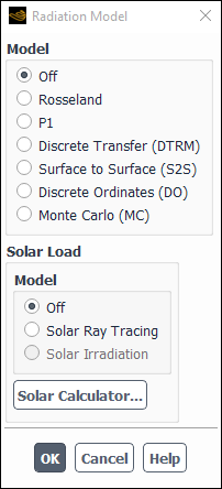
Important: Solar load is available in the 3D solver only, and can be used to model steady and unsteady flows.
The solar load model has two options: Solar Ray Tracing and Solar Irradiation. Solar Ray Tracing can be applied as a stand-alone solar loading model, or it can be used in conjunction with one of the Ansys Fluent radiation models. Solar Irradiation is available only when the Discrete Ordinates (DO) or Monte Carlo (MC)radiation model is enabled.
To set up the solar load model, perform the following steps:
Enable the solar load model in the Radiation Model Dialog Box.
To enable the solar ray tracing algorithm, select Solar Ray Tracing under Solar Load (Figure 16.49: The Radiation Model Dialog Box (With Solar Load Model Solar Ray Tracing Option)).
To enable the Solar Irradiation option, first select the DO or MC model, and then select Solar Irradiation under Solar Load (Figure 16.50: The Radiation Model Dialog Box (with Solar Load Model Solar Irradiation Option)).
When using the non-gray DO or MC model, if the wavelengths of the specified bands do not cover the entire solar spectrum, a message is written to the console displaying what percentage of the full solar model has been covered. It is recommended that the full solar spectrum is considered.
When using the non-gray MC model, if you only specify one band then Fluent will automatically cover the entire solar spectrum
Define the solar parameters.
Enter values for the X, Y, and Z components of the Sun Direction Vector. Alternatively, you can choose to have this vector computed from the solar calculator by enabling the Use Direction Computed from Solar Calculator option.
Specify the illumination parameters.
Enter a value for Direct Solar Irradiation under Illumination Parameters. This parameter is the amount of energy per unit area in
 due to direct solar irradiation.
This value may depend on the time of year and the
clearness of the sky. Make your selection in the
drop-down list next to Direct Solar
Irradiation and either enter a
constant value, have the
value computed from the solar
calculator, or specify it using a
user-defined function. Note
that only compiled (not interpreted) UDFs can be
used to specify Direct Solar
Irradiation. (For more information on
writing solar intensity UDFs, see
due to direct solar irradiation.
This value may depend on the time of year and the
clearness of the sky. Make your selection in the
drop-down list next to Direct Solar
Irradiation and either enter a
constant value, have the
value computed from the solar
calculator, or specify it using a
user-defined function. Note
that only compiled (not interpreted) UDFs can be
used to specify Direct Solar
Irradiation. (For more information on
writing solar intensity UDFs, see DEFINE_SOLAR_INTENSITYin the Fluent Customization Manual.) For transient simulations, you have the additional option of specifying a time-dependent piecewise-linear and polynomial profile for direct solar irradiation.Enter a value for Diffuse Solar Irradiation for the DO model only, which is the amount of energy per unit area in
 due to diffuse solar irradiation.
This value may depend on the time of year, the
clearness of the sky, and also on ground
reflectivity. Make your selection in the drop-down
list next to Diffuse Solar
Irradiation and either enter a
constant value, have the
value computed from the solar
calculator, or specify it using a
user-defined function. Note
that only compiled (not interpreted) UDFs can be
used to specify Diffuse Solar
Irradiation. (For more information on
writing solar intensity UDFs, see
due to diffuse solar irradiation.
This value may depend on the time of year, the
clearness of the sky, and also on ground
reflectivity. Make your selection in the drop-down
list next to Diffuse Solar
Irradiation and either enter a
constant value, have the
value computed from the solar
calculator, or specify it using a
user-defined function. Note
that only compiled (not interpreted) UDFs can be
used to specify Diffuse Solar
Irradiation. (For more information on
writing solar intensity UDFs, see DEFINE_SOLAR_INTENSITYin the Fluent Customization Manual.) For transient simulations, you have the additional option of specifying a time-dependent piecewise-linear and polynomial profile for diffuse solar irradiation.If you are using the Solar Ray Tracing solar load model (Figure 16.49: The Radiation Model Dialog Box (With Solar Load Model Solar Ray Tracing Option)), then you will need to enter a value for Spectral Fraction. The spectral fraction is the fraction of incident solar radiation in the visible part of the solar radiation spectrum.

(16–15)
where
 is the visible incident solar
radiation, and
is the visible incident solar
radiation, and  is the total incident solar
radiation (visible plus infrared).
is the total incident solar
radiation (visible plus infrared).
Use the solar calculator to compute solar beam direction and irradiation.
Click in the Radiation Model dialog box to open the Solar Calculator dialog box (Figure 16.51: The Solar Calculator Dialog Box).
In the Solar Calculator dialog box, define the Global Position by the following parameters:
Enter a real number in degrees for Longitude. Values may range from
 to
to  where negative values indicate the
Western hemisphere and positive values indicate the
Eastern hemisphere.
where negative values indicate the
Western hemisphere and positive values indicate the
Eastern hemisphere.Enter a real number for Latitude in degrees. Values can range from
 (the South Pole) to
 (the North Pole), with
 defined as the equator.
Enter an integer for Timezone that is the local time zone in hours relative to Greenwich Mean Time (+-GMT). This value can range from
 to
to  .
.
Important: Note that you must specify all three Global Position parameters for the solar calculator.
Define the local Date and Time by the following parameters:
Enter an integer for Day and Month under Day of Year.
Enter an integer for Hour that ranges from
 to
to  under Time of
Day. Enter an integer or floating point
number for Minute.
under Time of
Day. Enter an integer or floating point
number for Minute.The time of day is based on a 24-hour clock:
 hours and
  minutes corresponds to 12:00 a.m.
and
minutes corresponds to 12:00 a.m.
and  hours
hours  min corresponds to 11:59.99 p.m.
For example, if the local time was 12:01:30 a.m.,
you would enter
min corresponds to 11:59.99 p.m.
For example, if the local time was 12:01:30 a.m.,
you would enter 0for Hour and1.5for Minute. If the local time was 4:17 p.m., you would enter16for Hour and17for Minute.
Define the Mesh Orientation as the vectors for North and East in the CFD mesh system of coordinates.
Select the appropriate Solar Irradiation Method. The Fair Weather Conditions is the default method.
Enter an integer for Sunshine Fraction (default =
 ).
).Click .
The solar calculator output parameters are computed and the results are reported in the console. The default values are shown below:
 Fair Weather Conditions:
  Sun Direction Vector: X: -0.0785396, Y: 0.170758, X: 0.982178
  Sunshine Fraction: 1
  Direct Normal Solar Irradiation (at Earth’s surface) [W/m^2]:
  881.635
  Diffuse Solar Irradiation - vertical surface: [W/m^2]:
  152.107
  Diffuse Solar Irradiation - horizontal surface: [W/m^2]:
  118.727
  Ground Reflected Solar Irradiation - vertical surface: [W/m^2]:
  96.4649
For transient simulations, enter the Time Steps Per Solar Load Update under Update Parameters. The number of time steps that you specify will direct the Ansys Fluent solver to update the solar load data for the specified flow-time intervals in the unsteady solution process.
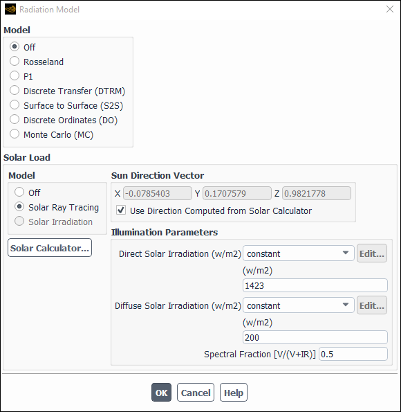
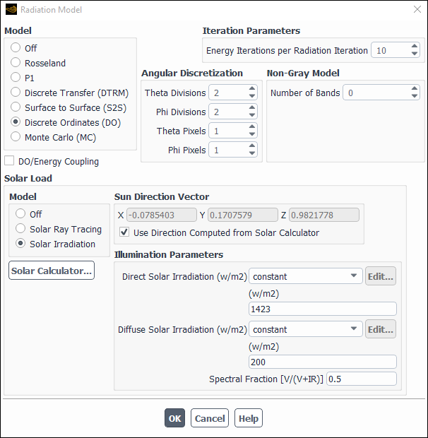
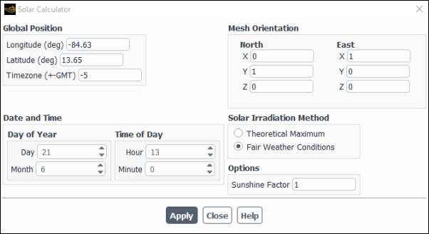
Once you have defined the solar parameters for the solar load model (Setting Up the Solar Load Model), you will need to set up boundary conditions for boundary zones that will participate in solar loading. The boundary condition dialog boxes can be opened by right-clicking the boundary name in the tree (under Setup/Boundary Conditions) and clicking Edit... in the menu that opens; alternatively, you can open them from the Boundary Conditions task page:
![]() Setup →
Setup → ![]() Boundary Conditions
Boundary Conditions
Note: Solar ray tracing is designed to be applied to your geometrical information, therefore, you must include every side of the external, or outer, enclosure/boundary for ray-tracing purposes, unless you expect that solar irradiation cannot enter through such boundaries. If you exclude any internal zone from the solar load computation, then this would mean that the resulting obstruction or blockage has been removed which would also be equivalent to a transparent surface. Excluded walls will also not participate in the computation of scattered energy by the solar load model and, therefore, do not gain any heat from scattered energy.
Set the boundary condition for each inlet and exit boundary zone that you want to include in solar loading.
Open the inlet or exit boundary condition dialog box (for example, Velocity Inlet) and click the Radiation tab (Figure 16.52: The Velocity Inlet Dialog Box).
Enable the Participates in Solar Ray Tracing option (this option is enabled for all boundary conditions by default). If you deactivate solar ray tracing by disabling this option the surface will be ignored and the solar ray will pass through it with no interaction, regardless of the boundary condition type.
Enter a value between
0and1for the Solar Transmissivity Factor. This will allow you to control the amount of solar irradiation entering the domain. By reducing the solar transmissivity factor from 1 to 0.5, you can effectively cut the total internal energy source entering the domain by half.Important: Note that the solar transmissivity factor is applied to both direct and diffuse solar irradiation components.
Click .
Set the boundary condition for each wall boundary zone that you want to include in solar loading.
Open a Wall boundary condition dialog box and click the Radiation tab.
Define the wall as opaque or semi-transparent. (An opaque wall will not allow any solar radiation to pass through it, while a semi-transparent surface will allow a portion of the solar radiation to pass through it.)
For an opaque wall, select opaque from the drop-down list for BC Type (Figure 16.53: The Wall Dialog Box). Then enable the Participates in Solar Ray Tracing option (this option is enabled for all boundary conditions by default) in the Solar Boundary Conditions group box and enter constant values for Direct Visible and Direct IR absorptivity. Note that if you deactivate solar ray tracing by disabling the Participates in Solar Ray Tracing option, the surface will be ignored and the solar ray will pass through it with no interaction, regardless of the boundary condition type.
Important: Absorption in the visible and infrared portions of the spectrum define the surface material for the opaque wall.
For a semi-transparent wall, select semi-transparent from the drop-down list for BC Type (Figure 16.54: The Wall Dialog Box). Then, enable the Participates in Solar Ray Tracing option (this option is enabled for all boundary conditions by default) in the Solar Boundary Conditions group box and enter constant values for Direct Visible, Direct IR, and Diffuse Hemispherical absorptivity and transmissivity. Note that if you deactivate solar ray tracing by disabling the Participates in Solar Ray Tracing option, the surface will be ignored and the solar ray will pass through it with no interaction, regardless of the boundary condition type.
Important: For semitransparent coupled walls, the solar ray tracing settings are defined on the original wall and not on the shadow wall.
Absorption and transmittance in the visible and infrared portions of the spectrum, as well as the “shading” formulation (Diffuse Hemispherical), define the surface material for a semi-transparent wall. These parameters are properties of the glazed unit and should be provided by the glazing manufacturer. The direct components are based on normal incident radiation (Ansys Fluent adjusts this for the actual angle of incidence). Most manufacturers present this information in a slightly different way so it may be necessary to seek guidance from the supplier. Another useful source of data can be found in the ASHRAE Fundamentals Handbook, chapter on Fenestration.
Click .
Set the boundary condition for each porous jump boundary zone that you want to include in solar loading. You can define the boundary such that it acts as a semi-transparent surface that will allow a portion of the solar radiation to pass through it, along with fluid flow. In this way you can represent a partial opening (for example, a grate, a grill, or a louver) that is a combination of gaps and (typically) opaque surfaces.
Open the Porous Jump boundary condition dialog box (Figure 16.55: The Porous Jump Dialog Box).
Define the Face Permeability, Porous Medium Thickness, Pressure-Jump Coefficient, and Thermal Contact Resistance as described in User Inputs for the Porous Jump Model.
Define the settings in the Solar Boundary Conditions group box.
Enable the Participates in Solar Ray Tracing option (this option is enabled for all boundary conditions by default). Note that if you deactivate solar ray tracing by disabling the Participates in Solar Ray Tracing option, the surface will be ignored and the solar ray will pass through it with no interaction, regardless of the boundary condition type.
Enter constant values (between 0 and 1) for Direct Visible and Direct IR in the Absorptivity group box. These values act as multipliers for the visible and infrared portions of the direct solar radiation spectrum, respectively, to account for the absorption of the porous jump.
Important: One reasonable way to estimate the Direct Visible and Direct IR absorptivity values for a grill, and so on, is to use the product of the obstructed area fraction and the surface absorptivity. For example, if 40% of the grill facial area is obstructed with grill slats, and the slats have a surface absorptivity of 0.7, you could estimate the absorptivity as being 0.28.
Enter constant values (between 0 and 1) for Direct Visible and Direct IR in the Transmissivity group box. These values act as multipliers for the visible and infrared portions of the direct solar radiation spectrum, respectively, to account for the transmissivity of the porous jump.
Important: One reasonable way to estimate the Direct Visible and Direct IR transmissivity values for a grill, and so on, is to use the open area fraction. For example, if a grill has openings between the slats that amount to 60% of the area, you could estimate the transmissivity as being 0.6.
Click .
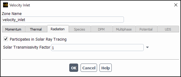
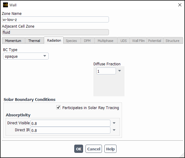
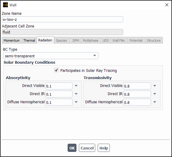

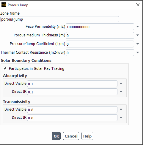
For Solar Irradiation, all boundary conditions are set up as normal for the DO or MC model, except that now you can select semi-transparent boundary surfaces that will provide a source of solar irradiation.
Open a Wall boundary condition dialog box and click the Radiation tab (Figure 16.56: The Wall Dialog Box Radiation tab with Solar Irradiation).
Select semi-transparent from the drop-down list for BC Type.
Enable the Use Beam Direction from Solar Load Model Settings option, under Solar BC Options, to have the values for beam direction applied from the Solar Load Model settings in the Radiation dialog box.
Important: Note that the sign of the beam direction that is needed for the DO or MC model is opposite the sun direction vector that is entered or derived from the solar parameters. The beam direction in the DO or MC model is the direction of external radiation (for example, radiation coming from the sun), while the sun direction vector in the solar load model points to the sun.
Enable the Use Irradiation from Solar Load Model Settings option to have the irradiation specified on the Radiation Model dialog box for the Solar Load model applied for direct and diffuse irradiation.
If selected while using the multiband approach for the DO or MC models, the direct and diffuse irradiation is calculated and applied in each band, according to the black body emission weighting factor.
When Use Irradiation from Solar Load Model Settings is enabled, the beam width will automatically be set to
 degrees - the angle subtended by the
sun.
degrees - the angle subtended by the
sun.Click .
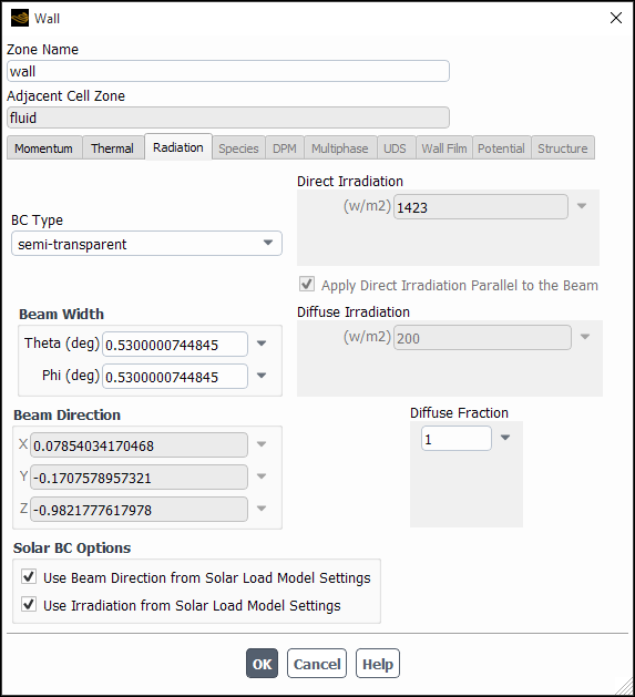
Ansys Fluent has provided some additional commands for solar load setup that are only available in the text interface. These commands are present in the following sections.
It is possible to direct Ansys Fluent to automatically save solar
load data to a generic file that you can examine or use in an external
program. This is done by executing the text command
autosave-solar-data from the text
interface. Note, this command is only available on Linux in serial mode
-t0.
define →
models →
radiation →
solar-parameters →
autosave-solar-data
Enter a value for the autosave solar data file frequency when prompted, in order to specify the frequency (in time steps) at which you want the solar load data written to a file. The default value is zero, which means that no automatic saving is performed.
Enter the filename, in quotations.
Choose to write file in binary format.
The text interface command for
autosave-solar-data for a file named
solar and a frequency of  is shown below:
 /define/models/radiation/solar-parameters> autosave-solar-data
  Autosave Solar Data File Frequency [0] 1
  Enter Filename [""] "solar"
When you are executing a transient simulation in serial or parallel Ansys Fluent version 18.2 or later and you want to read the solar load data file from a serial run performed in an earlier version, you can use the following text command:
define →
models →
radiation →
solar-parameters →
autoread-solar-data
Enter a value for the autoread solar data file frequency when prompted, in order to specify the frequency (in time steps) at which you want the solar load data read from the file generated during the serial run. The default value is zero, which means that no automatic reading is performed.
Enter the filename, in quotations.
The text interface command for
autoread-solar-data for a file named
solar and a frequency of  is shown below:
 /define/models/radiation/solar-parameters> autoread-solar-data
  Autoread Solar Data File Frequency [0] 1
  Enter Filename [""] "solar"
  Use Binary Format for Reading Data Files [yes]
When the solar load model is enabled, you can direct Ansys Fluent to align the camera direction with the sun position using the text interface command:
define →
models →
radiation →
solar-parameters →
sol-camera-pos
This command is useful when you are executing a transient simulation and you want to capture an image of your model with solar load parameters displayed (such as solar heat flux) as the sun position changes with time in order to create an animation. See Postprocessing Solar Load Quantities for details.
You can modify the default scattering fraction ( ) using the text interface command:
define →
models →
radiation →
solar-parameters →
scattering-fraction
The scattering fraction is the amount of direct radiation that has
been reflected from opaque surfaces (after entering through the
transparent surfaces) that will be considered to remain within the space
and be evenly distributed among all surfaces. The value is between
 and
and  .
.
The text interface command for specifying a
scattering-fraction of  is shown below:
 /define/models/radiation/solar-parameters> scattering-fraction
  Scattering Fraction [1] .5
You can direct Ansys Fluent to apply the solar load that is computed from the solar ray tracing algorithm to adjacent fluid cells by issuing the following command at the text interface:
define →
models →
radiation →
solar-parameters →
sol-adjacent-fluidcells
The text interface command is shown below:
 /define/models/radiation/solar-parameters> sol-adjacent-fluidcells
  Apply Solar Load on adjacent Fluid Cells? [no] y
This command allows you to apply solar loads to adjacent fluid cells only, even if solid or shell conduction zones are present. By applying the solar load on adjacent fluid cells, you are overruling the default order of the adjacent cell assignment in Ansys Fluent which is shell, solid, fluid.
You can modify the default value ( ) for the maximum quad tree refinement factor in the
solar ray tracing algorithm using the text command:
) for the maximum quad tree refinement factor in the
solar ray tracing algorithm using the text command:
define →
models →
radiation →
solar-parameters →
quad-tree-parameters
The text interface command is shown below, when a new maximum
refinement value of  is specified:
 /define/models/radiation/solar-parameters> quad-tree-parameters
  Maximum Quad-Tree Refinement [7] 10
You can modify the default value ( ) for the ground reflectivity using the text
command:
) for the ground reflectivity using the text
command:
define →
models →
radiation →
solar-parameters →
ground-reflectivity
Ground reflectivity  (Equation 16–14) includes the
contribution of reflected solar radiation from ground surfaces. It is
treated as part of the total diffuse solar irradiation when the solar
calculator is used in conjunction with the
(Equation 16–14) includes the
contribution of reflected solar radiation from ground surfaces. It is
treated as part of the total diffuse solar irradiation when the solar
calculator is used in conjunction with the Diffuse Solar
Irradiation illumination parameter. The default value
is  .
.
 /define/models/radiation/solar-parameters> ground-reflectivity
  Ground Reflectivity [0.2] 0.5
For consistency with cases set up previous to Fluent 2019 r1, you can use the following command so that the complete solar load is applied to the first band only.
define →
models →
radiation →
apply-full-solar-irradiation?
  /define/models/radiation/apply-full-solar-irradiation?
Apply full solar irradiation to first band? [no] yes
Some solar load commands that are available in the graphical user interface are also made available in the text interface. For example, you can turn the solar load model on using the text command:
define →
models →
radiation →
solar?
You can also enter the solar calculator parameters in the text interface by executing the command:
define →
models →
radiation →
solar-calculator
Once invoked, you will be prompted to enter the solar calculator input parameters.
To set the illumination parameters, select this option from the
solar-parameters menu:
define →
models →
radiation →
solar-parameters →
illumination-parameters
And finally, you can direct Ansys Fluent to compute the solar load on demand, by issuing the text command:
define →
models →
radiation →
solar-parameters →
sol-on-demand
When the command is initiated, the solar data are written to the console.
The following solar load quantities can be used to visualize the illuminated areas and shadows created by solar radiation.
solar heat flux (that is, sum of visible and IR absorbed solar flux on opaque walls)
absorbed visible and IR solar flux (semi-transparent walls and porous jump boundaries only)
reflected visible and IR solar flux (semi-transparent walls and porous jump boundaries only)
transmitted visible and IR solar flux (semi-transparent walls and porous jump boundaries only)
These quantities are available for postprocessing of solar loading at wall
boundaries and can be displayed as contours of Wall Fluxes
in the Contours dialog box. For steady-state simulations,
the solar flux data is computed at solution initialization and is available for
postprocessing. You can also compute the solar load at any time during your
Ansys Fluent session, after you have set up the model and applied boundary
conditions. To compute the solar load on demand, you can issue the
sol-on-demand command in the text interface (see
Additional Text Interface Commands for details).
Solar heat flux, for example, can be displayed for surfaces using the Contours dialog box. A sample dialog box is shown below (Figure 16.57: The Contours Dialog Box).
![]() Results → Graphics
→ Contours
Results → Graphics
→ Contours
![]() New...
New...
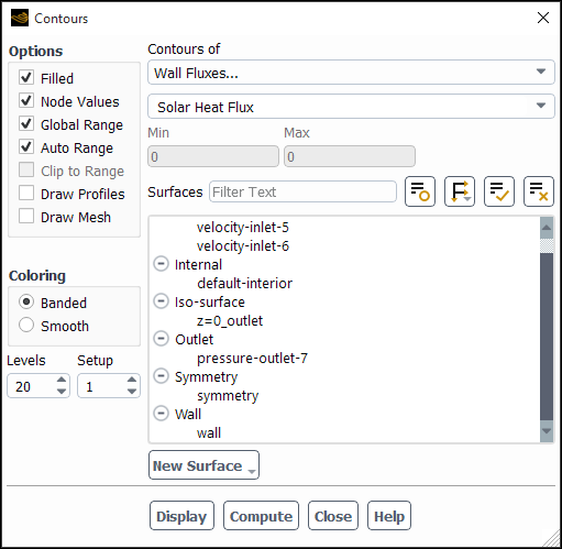
The solar camera alignment command is useful when you want to take timed pictures of solar loading effects of your model during transient simulations, and later create animations of the image files using an external program. Follow the procedure below.
Read (or set up) your transient case file in Ansys Fluent.
Set up the automatic execution of solution commands in the Execute Commands dialog box that will: 1) display solar load parameter graphics, 2) re-position the solar camera such that the view is aligned with the instantaneous sun direction, and 3) generate a picture image file (
.tiff) during the solution process in the Execute Commands dialog box. Solution →
Calculation Activities →
Execute Commands
Edit...
Initialize and run the solution.
Animate the
.tifffiles using an external animation tool.
The following commands entered in the Execute
Commands dialog box will direct Ansys Fluent to display
contours of solar heat flux, align the camera with the current direction of
the sun, and then generate a picture image file
(.tiff) of the solar heat flux contour every
300 time steps during the unsteady simulation. See Figure 16.58: The Execute Commands Dialog Box.
 /di/cont solar-heat-flux ,,
 /def/mod/rad/solar-para/sol-camera-pos
 /di/hc "flux-%t.tiff"
Ansys Fluent provides some additional solar load variables that you can use for postprocessing when your model includes solar ray tracing. You can generate graphical plots or alphanumeric reports of the following variables:
In the Wall Fluxes... category:
Solar Heat Flux
Transmitted Visible Solar Flux (semi-transparent walls and porous jump boundaries)
Transmitted IR Solar Flux (semi-transparent walls and porous jump boundaries)
Reflected Visible Solar Flux (semi-transparent walls and porous jump boundaries)
Reflected IR Solar Flux (semi-transparent walls and porous jump boundaries)
Absorbed Visible Solar Flux (semi-transparent walls and porous jump boundaries)
Absorbed IR Solar Flux (semi-transparent walls and porous jump boundaries)
See Field Function Definitions for their definitions.