


The Boundary Conditions task page allows you to set the type of a boundary and display other dialog boxes to set the boundary condition parameters for each boundary.
Controls
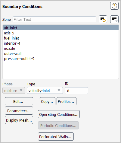
- Zone
contains a selectable list of boundary zones from which you can select the zone of interest. You can check a zone type by using the mouse probe (see Controlling the Mouse Button Functions) on the displayed physical mesh. This feature is particularly handy if you are setting up a problem for the first time, or if you have two or more boundary zones of the same type and you want to determine the zone IDs. To do this you must first display the mesh with the Mesh Display Dialog Box. Then click the boundary zone with the right (select) mouse button. Ansys Fluent will print the zone ID and type of that boundary zone in the console window.
- Phase
specifies the phase for which conditions at the selected boundary Zone are being set. This item appears if the VOF, mixture, or Eulerian multiphase model is being used. See Defining Multiphase Cell Zone and Boundary Conditions for details.
- Type
contains a drop-down list of boundary condition types for the selected zone. The list contains all possible types to which the zone can be changed.
Important: Note that you cannot use this method to change zone types to or from the periodic type, since additional restrictions exist for this boundary type. Creating Periodic Zones and Interfaces explains how to create and uncouple periodic zones.
- ID
displays the zone ID number of the selected zone. (This is for informational purposes only; you cannot edit this number.)
- Edit...
opens the appropriate dialog box for setting the boundary conditions for that particular boundary type.
- Copy...
opens the Copy Conditions Dialog Box, which allows you to copy boundary conditions from one zone to other zones of the same type. See Copying Cell Zone and Boundary Conditions for details.
- Profiles...
opens the Profiles Dialog Box.
- Parameters...
opens the Parameters Dialog Box.
- Operating Conditions...
opens the Operating Conditions Dialog Box.
- Display Mesh...
opens the Mesh Display Dialog Box.
- Periodic Conditions...
opens the Periodic Conditions Dialog Box.
- Perforated Walls...
opens the Perforated Walls Dialog Box.
For additional information, see the following sections:
- 51.7.1. Axis Dialog Box
- 51.7.2. Degassing Dialog Box
- 51.7.3. Exhaust Fan Dialog Box
- 51.7.4. Fan Dialog Box
- 51.7.5. Inlet Vent Dialog Box
- 51.7.6. Intake Fan Dialog Box
- 51.7.7. Interface Dialog Box
- 51.7.8. Interior Dialog Box
- 51.7.9. Mass-Flow Inlet Dialog Box
- 51.7.10. Mass-Flow Outlet Dialog Box
- 51.7.11. Outflow Dialog Box
- 51.7.12. Outlet Vent Dialog Box
- 51.7.13. Overset Dialog Box
- 51.7.14. Periodic Dialog Box
- 51.7.15. Porous Jump Dialog Box
- 51.7.16. Pressure Far-Field Dialog Box
- 51.7.17. Pressure Inlet Dialog Box
- 51.7.18. Pressure Outlet Dialog Box
- 51.7.19. Radiator Dialog Box
- 51.7.20. RANS/LES Interface Dialog Box
- 51.7.21. Symmetry Dialog Box
- 51.7.22. Velocity Inlet Dialog Box
- 51.7.23. Wall Dialog Box
- 51.7.24. Periodic Conditions Dialog Box
- 51.7.25. Perforated Walls Dialog Box
The Axis dialog box can be used to modify the name of an axis zone; there are no conditions to be set. It is opened from the Boundary Conditions Task Page. See Axis Boundary Conditions for information about axis boundaries.
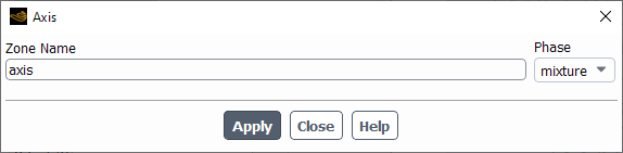
Controls
- Zone Name
sets the name of the zone.
- Phase
displays the name of the phase. This item appears if the VOF, mixture, or Eulerian multiphase model is being used.
The Degassing dialog box can be used to modify the name of a degassing zone; there are no conditions to be set. It is opened from the Boundary Conditions Task Page. See Degassing Boundary Conditions for information about axis boundaries.

Controls
- Zone Name
sets the name of the zone.
- Phase
displays the name of the phase.
The Exhaust Fan dialog box sets the boundary conditions for an exhaust fan zone. It is opened from the Boundary Conditions Task Page. See Inputs at Exhaust Fan Boundaries for details about defining the items below.
Important: This feature offers reduced functionality when running Fluent under the Pro capability level.

Controls
- Zone Name
sets the name of the zone.
- Phase
displays the name of the phase. It appears only for multiphase flows.
- Momentum
contains the momentum parameters.
- Backflow Reference Frame
specify whether backflow temperature, pressure, and flow directions are in the Absolute or Relative to the Adjacent Cell Zone reference frame.
- Gauge Pressure
sets the gauge pressure at the outlet boundary.
- Backflow Direction Specification Method
sets the direction of the inflow stream should the flow reverse direction. You can choose Direction Vector, Normal to Boundary,or From Neighboring Cell.
- Coordinate System
contains a drop-down list for selecting the coordinate system. You can choose Cartesian, Cylindrical, or Local Cylindrical. This option is available only when Direction Vector is selected from the Backflow Direction Specification Method drop-down list.
- X-, Y-, Z-Component of Flow Direction
allows you to specify the velocity components in x, y, and z directions respectively. This option is available when Cartesian is selected for the Coordinate System.
- Radial-, Tangential-, Axial-Component of Flow Direction
set the direction of the flow at the boundary. These items will appear for 2D axisymmetric cases, or for 3D cases for which the selected Coordinate System is Cylindrical or Local Cylindrical.
- Backflow Pressure Specification
specifies how the pressure is calculated under backflow conditions. If you select Static Pressure, the Gauge Pressure is directly imposed as the boundary face pressure; if you select Total Pressure, the Gauge Pressure will be combined with a dynamic contribution that is based on the velocity in the adjacent cell zone.
- Pressure Jump
specifies the rise in pressure across the fan. See Specifying the Pressure Jump for details.
- Axis Origin
sets the X, Y, and Z coordinates of the origin of the local cylindrical coordinate system.
- Axis Direction
sets the X, Y, and Z components of the direction of the local cylindrical coordinate system.
- Turbulence
displays the turbulence parameters.
- Specification Method
specifies which method will be used to define the turbulence parameters. You can choose K and Epsilon (
 -
-  models and RSM only), K and Omega
(
models and RSM only), K and Omega
( -
-  models only), Intensity and Length Scale,
Intensity and Viscosity Ratio, Intensity and Hydraulic
Diameter, Modified Turbulent Viscosity (Spalart-Allmaras
model only), or Turbulent Viscosity Ratio (Spalart-Allmaras model
only). See Determining Turbulence Parameters for information about the inputs for each
of these methods. (This item will appear only for turbulent flow calculations.)
models only), Intensity and Length Scale,
Intensity and Viscosity Ratio, Intensity and Hydraulic
Diameter, Modified Turbulent Viscosity (Spalart-Allmaras
model only), or Turbulent Viscosity Ratio (Spalart-Allmaras model
only). See Determining Turbulence Parameters for information about the inputs for each
of these methods. (This item will appear only for turbulent flow calculations.)- Backflow Turbulent Kinetic Energy, Backflow Turbulent Dissipation Rate
set values for the turbulence kinetic energy
 and its dissipation rate
  . These items will appear if you choose K and
Epsilon as the Specification Method.
. These items will appear if you choose K and
Epsilon as the Specification Method.- Backflow Turbulent Kinetic Energy, Backflow Specification Dissipation Rate
set values for the turbulence kinetic energy
 and its specific dissipation rate
  . These items will appear if you choose K and
Omega as the Specification Method.
. These items will appear if you choose K and
Omega as the Specification Method.- Backflow Turbulent Intensity, Backflow Turbulent Length Scale
set values for turbulence intensity
 and turbulence length scale
  . These items will appear if you choose Intensity and Length
Scale as the Specification Method.
. These items will appear if you choose Intensity and Length
Scale as the Specification Method.- Backflow Turbulent Intensity, Backflow Turbulent Viscosity Ratio
set values for turbulence intensity
 and turbulent viscosity ratio
  . These items will appear if you choose Intensity and
Viscosity Ratio as the Specification Method.
. These items will appear if you choose Intensity and
Viscosity Ratio as the Specification Method.- Backflow Turbulent Intensity, Backflow Hydraulic Diameter
set values for turbulence intensity
 and hydraulic diameter
  . These items will appear if you choose Intensity and
Hydraulic Diameter as the Specification Method.
. These items will appear if you choose Intensity and
Hydraulic Diameter as the Specification Method.- Backflow Modified Turbulent Viscosity
sets the value of the backflow modified turbulent viscosity
 . This item will appear if you choose Modified Turbulent
Viscosity as the Specification Method.
. This item will appear if you choose Modified Turbulent
Viscosity as the Specification Method.- Backflow Turbulent Viscosity Ratio
sets the value of the backflow turbulent viscosity ratio
 . This item will appear if you choose Turbulent Viscosity
Ratio as the Specification Method.
. This item will appear if you choose Turbulent Viscosity
Ratio as the Specification Method.- Reynolds-Stress Specification Method
specifies which method will be used to determine the backflow Reynolds stress boundary conditions when the Reynolds stress turbulence model is used. You can choose either K or Turbulence Intensity or Reynolds-Stress Components. If you choose the former, Ansys Fluent will compute the Reynolds stresses for you. If you choose the latter, you will explicitly specify the Reynolds stresses yourself. See Reynolds Stress Model for details. (This item will appear only for RSM turbulent flow calculations.)
- Backflow UU, VV, WW, UV, VW, UW Reynolds Stresses
specify the backflow Reynolds stress components when Reynolds-Stress Components is chosen as the Reynolds-Stress Specification Method.
- Thermal
contains the thermal parameters. This parameter is available only when the energy equation is turned on.
- Backflow Total Temperature
sets the total temperature of the inflow stream should the flow reverse direction.
- Radiation
contains the boundary conditions for the radiation model at the exhaust fan.
- External Black Body Temperature Method, Internal Emissivity
set the radiation boundary conditions when you are using the P-1, DTRM, DO, S2S, or MC models for radiation heat transfer. See Defining Boundary Conditions for Radiation for details.
- Participates in Solar Ray Tracing
specifies whether or not the fan participates in solar ray tracing.
- Solar Transmissivity Factor
specifies a multiplier (ranging from 0 to 1) that is applied to the solar irradiation entering the domain through the fan.
- Participates in View Factor Calculation
specifies whether or not the fan participates in the view factor calculation as part of the S2S radiation model. This parameter is available only if you select the Surface to Surface radiation model.
- Species
contains the species parameters.
- Specify Species in Mole Fractions
allows you to specify the species in mole fractions rather than mass fractions.
- Mean Mixture Fraction, Mixture Fraction Variance
set inlet values for the PDF mixture fraction and its variance. (These items will appear only if you are using the non-premixed or partially premixed combustion model.)
- Secondary Mean Mixture Fraction, Secondary Mixture Fraction Variance
set inlet values for the secondary mixture fraction and its variance. (These items will appear only if you are using the non-premixed or partially premixed combustion model with two mixture fractions.)
- Species Mass Fractions
contains inputs for the mass fractions of defined species. See Defining Cell Zone and Boundary Conditions for Species for details about these inputs. These items will appear only if you are modeling non-reacting multi-species flow or you are using the finite-rate reaction formulation.
- Backflow Progress Variable
sets the value of the progress variable for premixed turbulent combustion. See Setting Boundary Conditions for the Progress Variable for details.
This item will appear only if the premixed or partially premixed combustion model is used.
- DPM
contains the discrete phase parameters. This tab is available only if you have defined at least one injection.
- Discrete Phase BC Type
sets the way that the discrete phase behaves with respect to the boundary. This item appears when one or more injections have been defined.
- reflect
rebounds the particle off the boundary with a change in its momentum as defined by the coefficient of restitution (see Particle Reflection at Wall in the Fluent Theory Guide).
- trap
terminates the trajectory calculations and records the fate of the particle as "trapped". In the case of evaporating droplets, their entire mass instantaneously passes into the vapor phase and enters the cell adjacent to the boundary. See Figure 24.40: “Trap” Boundary Condition for the Discrete Phase.
- escape
reports the particle as having "escaped" when it encounters the boundary. Trajectory calculations are terminated. See Figure 24.41: “Escape” Boundary Condition for the Discrete Phase.
- reinject
reintroduces the particle into the domain when it reaches a certain domain boundary (for example, outlet). This item appears when one or more injections have been defined and Unsteady Particle Tracking is enabled in the Discrete Phase Model dialog box. See The reinject Boundary Condition for details.
- wall-jet
indicates that the direction and velocity of the droplet particles are given by the resulting momentum flux, which is a function of the impingement angle. See Figure 12.6: "Wall Jet" Boundary Condition for the Discrete Phase in the Theory Guide.
- user-defined
specifies a user-defined function to define the discrete phase boundary condition type.
- Discrete Phase BC Function
sets the user-defined function from the drop-down list.
- Multiphase
contains the multiphase parameters.
- Backflow Granular Temperature
specifies temperature for the solids phase and is proportional to the kinetic energy of the random motion of the particles.
- Volume Fraction Specification Method
sets the method used to specify the volume fraction of the secondary phase selected in the Boundary Conditions Task Page. This section of the dialog box will appear when one of the multiphase models is being used. See Defining Multiphase Cell Zone and Boundary Conditions for details.
- Backflow Volume Fraction
specifies the volume fraction of the secondary phase as a constant, profile, of UDF function.
- From Neighboring Cell
calculates the volume fraction from the neighboring cells.
- Potential
displays the boundary conditions for the electric potential field. This tab is available only if you have enabled either the Electric Potential model or the Electrochemical reaction model in the Species Dialog Box.
- Potential Boundary Condition
is a drop-down list of available potential boundary condition types for the potential generated by electron current: Specified Flux and Specified Value. For the Specified Flux boundary condition, you will need to specify Current Density at the wall. For the Specified Value boundary condition, you will need to specify Potential at the wall.
- Electrolyte Potential Boundary Condition
is a drop-down list of available boundary condition types for the potential generated by ionic current. This item is similar to the Potential Boundary Condition drop-down list described above and is available only for the Electrolysis and H2 Pump model.
- UDS
contains the UDS parameters.
- User-Defined Scalar Boundary Condition
appears only if user-defined scalars are specified.
- User Scalar n
specifies whether the scalar is a specified flux or a specified value.
- User-Defined Scalar Boundary Value
appears only if user-defined scalars are specified.
- User Scalar n
specifies the value of the scalar.
The Fan dialog box sets the boundary conditions for a fan zone. It is opened from the Boundary Conditions Task Page. See User Inputs for Fans for details about the items below.
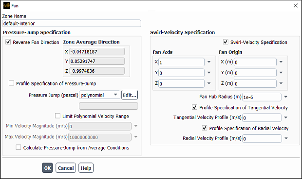
Controls
- Zone Name
sets the name of the zone.
- Pressure-Jump Specification
contains inputs that define the pressure jump across the fan.
- Reverse Fan Direction
sets the fan flow direction relative to the zone direction. If Zone Average Direction is pointing in the direction you want the fan to blow, do not select Reverse Flow; if it is pointing in the opposite direction, select Reverse Flow.
- Zone Average Direction
displays the (face-averaged) direction vector for the zone as an aid in determining whether or not you want to select Reverse Flow.
- Profile Specification of Pressure-Jump
enables the use of a boundary profile or user-defined function for the pressure jump specification. See Profiles or the Fluent Customization Manual for details. When this option is enabled, Pressure Jump Profile will appear in the dialog box and the next four items below it will not.
- Pressure Jump Profile
contains a drop-down list from which you can select a boundary profile or a user-defined function for the pressure jump definition. This item will appear if you enable Profile Specification of Pressure-Jump.
- Pressure-Jump
specifies the pressure-jump as a constant value or as a polynomial, piecewise-linear, or piecewise-polynomial function of velocity. See Defining the Pressure Jump for details.
- Limit Polynomial Velocity Range
limits the minimum and maximum velocity magnitudes used to calculate the pressure jump when it is defined as a function of velocity.
- Min Velocity Magnitude, Max Velocity Magnitude
specify the minimum and maximum values to which the velocity magnitude is limited (when the Limit Polynomial Velocity Range option is enabled).
- Calculate Pressure-Jump from Average Conditions
enables the option to use the mass-averaged velocity normal to the fan to determine a single pressure-jump value for all faces in the fan zone.
- Discrete Phase BC Type
sets the way that the discrete phase behaves with respect to the boundary. This item appears when one or more injections have been defined.
- interior
allows the particles to pass through the boundary.
- reflect
rebounds the particle off the boundary with a change in its momentum as defined by the coefficient of restitution. (See Particle Reflection at Wall in the Fluent Theory Guide.)
- trap
terminates the trajectory calculations and records the fate of the particle as "trapped". In the case of evaporating droplets, their entire mass instantaneously passes into the vapor phase and enters the cell adjacent to the boundary. See Figure 24.40: “Trap” Boundary Condition for the Discrete Phase.
- escape
reports the particle as having "escaped" when it encounters the boundary. Trajectory calculations are terminated. See Figure 24.41: “Escape” Boundary Condition for the Discrete Phase.
- reinject
reintroduces the particle into the domain when it reaches a certain domain boundary (for example, outlet). This item appears when one or more injections have been defined and Unsteady Particle Tracking is enabled in the Discrete Phase Model dialog box. See The reinject Boundary Condition for details.
- wall-jet
indicates that the direction and velocity of the droplet particles are given by the resulting momentum flux, which is a function of the impingement angle. See Figure 12.6: "Wall Jet" Boundary Condition for the Discrete Phase in the Theory Guide.
- user-defined
specifies a user-defined function to define the discrete phase boundary condition type.
- Discrete Phase BC Function
sets the user-defined function from the drop-down list.
- Swirl-Velocity Specification
contains inputs for the specification of fan swirl velocity. This section of the dialog box appears only for 3D models.
- Swirl-Velocity Specification
enables the specification of a swirl velocity for the fan.
- Fan Axis
sets the direction vector for the fan’s axis of rotation.
- Fan Origin
sets the origin in the global coordinate system through which the fan rotation axis passes.
- Fan Hub Radius
set the radius of the hub. The default is 1e-6 to avoid division by zero in the polynomial.
- Profile Specification of Tangential Velocity
enables the use of a boundary profile or user-defined function for the tangential velocity specification. See Profiles or the Fluent Customization Manual for details. When this option is enabled, Tangential Velocity Profile will appear in the dialog box and Tangential-Velocity Polynomial Coefficients will not.
- Tangential Velocity Profile
contains a drop-down list from which you can select a boundary profile or a user-defined function for the definition of the tangential velocity. This item will appear if you enable Profile Specification of Tangential Velocity.
- Tangential-Velocity Polynomial Coefficients
sets the coefficients for the tangential velocity polynomial. Separate the coefficients by spaces.
- Profile Specification of Radial Velocity
enables the use of a boundary profile or user-defined function for the radial velocity specification. See Profiles or the Fluent Customization Manual for details. When this option is enabled, Radial Velocity Profile will appear in the dialog box and Radial-Velocity Polynomial Coefficients will not.
- Radial Velocity Profile
contains a drop-down list from which you can select a boundary profile or a user-defined function for the definition of the radial velocity. This item will appear if you enable Profile Specification of Radial Velocity.
- Radial-Velocity Polynomial Coefficients
sets the coefficients for the radial velocity polynomial. Separate the coefficients by spaces.
The Inlet Vent dialog box sets the boundary conditions for an inlet vent zone. It is opened from the Boundary Conditions Task Page. See Inputs at Inlet Vent Boundaries for details about defining the items below.
Important: This feature offers reduced functionality when running Fluent under the Pro capability level.
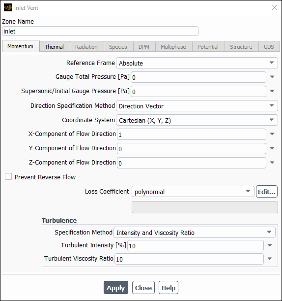
Controls
- Zone Name
sets the name of the zone.
- Momentum
contains the momentum parameters.
- Reference Frame
specifies the reference frame for the inlet vent. If the cell zone adjacent to the inlet vent is moving, you can choose to specify relative or absolute velocities by selecting Relative to Adjacent Cell Zone or Absolute in the Reference Frame drop-down list.
- Gauge Total Pressure
sets the gauge total (or stagnation) pressure of the inflow stream. If you are using moving reference frames, see Defining Total Pressure and Temperature for information about relative and absolute total pressure.
- Supersonic/Initial Gauge Pressure
sets the static pressure on the boundary when the flow becomes (locally) supersonic. It is also used to compute initial values for pressure, temperature, and velocity if the inlet vent boundary condition is selected for computing initial values (see Initializing the Entire Flow Field Using Standard Initialization).
- Direction Specification Method
specifies the method you will use to define the flow direction. If you choose Direction Vector, you will define the flow direction components, and if you choose Normal to Boundary no inputs are required. See Defining the Flow Direction for information on specifying flow direction.
- Coordinate System
specifies whether Cartesian, Cylindrical, Local Cylindrical, Local Cylindrical Swirl vector components will be specified. This item will appear only for 3D cases in which you have selected Direction Vector as the Direction Specification Method.
- X,Y,Z-Component of Flow Direction
set the direction of the flow at the inlet boundary. These items will appear if the selected Coordinate System is Cartesian or the model is 2D non-axisymmetric.
- Radial, Tangential, Axial Component of Flow Direction
set the direction of the flow at the inlet boundary. These items will appear for 2D axisymmetric cases, or for 3D cases for which the selected Coordinate System is Cylindrical or Local Cylindrical.
- Axis Origin
sets the X, Y, and Z coordinates of the origin of the local cylindrical coordinate system.
- Axis Direction
sets the X, Y, and Z components of the direction of the local cylindrical coordinate system.
- Loss-Coefficient
sets the non-dimensional loss coefficient used to compute the pressure drop. See Specifying the Loss Coefficient for details.
- Turbulence
lists the turbulence parameters.
- Specification Method
specifies which method will be used to define the turbulence parameters. You can choose K and Epsilon (
 -
-  models and RSM only), K and Omega
(
models and RSM only), K and Omega
( -
-  models only), Intensity and Length Scale,
Intensity and Viscosity Ratio, Intensity and Hydraulic
Diameter, Modified Turbulent Viscosity (Spalart-Allmaras
model only), or Turbulent Viscosity Ratio (Spalart-Allmaras model
only). See Determining Turbulence Parameters for information about the inputs for each
of these methods. (This item will appear only for turbulent flow calculations.)
models only), Intensity and Length Scale,
Intensity and Viscosity Ratio, Intensity and Hydraulic
Diameter, Modified Turbulent Viscosity (Spalart-Allmaras
model only), or Turbulent Viscosity Ratio (Spalart-Allmaras model
only). See Determining Turbulence Parameters for information about the inputs for each
of these methods. (This item will appear only for turbulent flow calculations.)- Turbulent Kinetic Energy, Turbulent Dissipation Rate
set values for the turbulence kinetic energy
 and its dissipation rate
  . These items will appear if you choose K and
Epsilon as the Specification Method.
. These items will appear if you choose K and
Epsilon as the Specification Method.- Turbulent Kinetic Energy, Specific Dissipation Rate
set values for the turbulence kinetic energy
 and its specific dissipation rate
  . These items will appear if you choose K and
Omega as the Specification Method.
. These items will appear if you choose K and
Omega as the Specification Method.- Turbulence Intensity, Turbulence Length Scale
set values for turbulence intensity
 and turbulence length scale
  . These items will appear if you choose Intensity and Length
Scale as the Specification Method.
. These items will appear if you choose Intensity and Length
Scale as the Specification Method.- Turbulence Intensity, Turbulent Viscosity Ratio
set values for turbulence intensity
 and turbulent viscosity ratio
  . These items will appear if you choose Intensity and
Viscosity Ratio as the Specification Method.
. These items will appear if you choose Intensity and
Viscosity Ratio as the Specification Method.- Turbulence Intensity, Hydraulic Diameter
set values for turbulence intensity
 and hydraulic diameter
  . These items will appear if you choose Intensity and
Hydraulic Diameter as the Specification Method.
. These items will appear if you choose Intensity and
Hydraulic Diameter as the Specification Method.- Modified Turbulent Viscosity
sets the value of the modified turbulent viscosity
 . This item will appear if you choose Modified Turbulent
Viscosity as the Specification Method.
. This item will appear if you choose Modified Turbulent
Viscosity as the Specification Method.- Turbulent Viscosity Ratio
sets the value of the turbulent viscosity ratio
 . This item will appear if you choose Turbulent Viscosity
Ratio as the Specification Method.
. This item will appear if you choose Turbulent Viscosity
Ratio as the Specification Method.- Reynolds-Stress Specification Method
specifies which method will be used to determine the Reynolds stress boundary conditions when the Reynolds stress turbulence model is used. You can choose either K or Turbulence Intensity or Reynolds-Stress Components. If you choose the former, Ansys Fluent will compute the Reynolds stresses for you. If you choose the latter, you will explicitly specify the Reynolds stresses yourself. See Reynolds Stress Model for details. (This item will appear only for RSM turbulent flow calculations.)
- UU, VV, WW, UV, VW, UW Reynolds Stresses
specify the Reynolds stress components when Reynolds-Stress Components is chosen as the Reynolds-Stress Specification Method.
- Thermal
contains the thermal parameters.
- Total Temperature
sets the total temperature of the inflow stream. If you are using moving reference frames, see Defining Total Pressure and Temperature for information about relative and absolute total temperature.
- Radiation
contains the radiation parameters.
- External Black Body Temperature Method, Internal Emissivity
set the radiation boundary conditions when you are using the P-1, DTRM, DO, S2S, or MC models for radiation heat transfer. See Defining Boundary Conditions for Radiation for details.
- Participates in Solar Ray Tracing
specifies whether or not the inlet vent participates in solar ray tracing.
- Solar Transmissivity Factor
specifies a multiplier (ranging from 0 to 1) that is applied to the solar irradiation entering the domain through the inlet vent.
- Participates in View Factor Calculation
specifies whether or not the inlet vent participates in the view factor calculation as part of the S2S radiation model. This parameter is available only if you select the Surface to Surface radiation model.
- Species
contains the species parameters.
- Specify Species in Mole Fractions
allows you to specify the species in mole fractions rather than mass fractions.
- Species Mass Fractions
contains inputs for the mass fractions of defined species. See Defining Cell Zone and Boundary Conditions for Species for details about these inputs. (These items will appear only if you are modeling non-reacting multi-species flow or you are using the finite-rate reaction formulation.)
- Mean Mixture Fraction, Mixture Fraction Variance
set inlet values for the PDF mixture fraction and its variance. (These items will appear only if you are using the non-premixed or partially premixed combustion model.)
- Secondary Mean Mixture Fraction, Secondary Mixture Fraction Variance
set inlet values for the secondary mixture fraction and its variance. (These items will appear only if you are using the non-premixed or partially premixed combustion model with two mixture fractions.)
- Progress Variable
sets the value of the progress variable for premixed turbulent combustion. See Setting Boundary Conditions for the Progress Variable for details.
This item will appear only if the premixed or partially premixed combustion model is used.
- DPM
contains the discrete phase parameters.
- Discrete Phase BC Type
sets the way that the discrete phase behaves with respect to the boundary. This item appears when one or more injections have been defined.
- reflect
rebounds the particle off the boundary with a change in its momentum as defined by the coefficient of restitution. (See Particle Reflection at Wall in the Fluent Theory Guide.)
- trap
terminates the trajectory calculations and records the fate of the particle as "trapped". In the case of evaporating droplets, their entire mass instantaneously passes into the vapor phase and enters the cell adjacent to the boundary. See Figure 24.40: “Trap” Boundary Condition for the Discrete Phase.
- escape
reports the particle as having "escaped" when it encounters the boundary. Trajectory calculations are terminated. See Figure 24.41: “Escape” Boundary Condition for the Discrete Phase.
- reinject
reintroduces the particle into the domain when it reaches a certain domain boundary (for example, outlet). This item appears when one or more injections have been defined and Unsteady Particle Tracking is enabled in the Discrete Phase Model dialog box. See The reinject Boundary Condition for details.
- wall-jet
indicates that the direction and velocity of the droplet particles are given by the resulting momentum flux, which is a function of the impingement angle. See Figure 12.6: "Wall Jet" Boundary Condition for the Discrete Phase in the Theory Guide.
- user-defined
specifies a user-defined function to define the discrete phase boundary condition type.
- Discrete Phase BC Function
sets the user-defined function from the drop-down list.
- Multiphase
contains the multiphase parameters.
- Granular Temperature
specifies temperature for the solids phase and is proportional to the kinetic energy of the random motion of the particles.
- Volume Fraction
specifies the volume fraction of the secondary phase selected in the Boundary Conditions Task Page. This section of the dialog box will appear when one of the multiphase models is being used. See Defining Multiphase Cell Zone and Boundary Conditions for details.
- Open Channel
is available when the VOF model with open channel flow is enabled.
- Secondary Phase for Inlet
is where the specified parameters are valid only for one secondary phase. In case of a three-phase flow, select the corresponding secondary phase from this list. This appears when Open Channel is enabled.
- Flow Specification Method
allows you to select the type of flow. You can choose Free Surface Level and Velocity, Total Height and Velocity, or Free Surface Level and Total Height. This appears when Open Channel is enabled.
- Free Surface Level
can be determined using the absolute value of height from the free surface to the origin in the direction of gravity, or by applying the correct sign based on whether the free surface level is above or below the origin.
- Total Height
is used as an option for describing the flow. It is given by Equation 26–12.
- Bottom Level
is valid only for shallow waves. The bottom level is used for calculating the liquid height.
- Velocity Magnitude
sets the magnitude of the velocity vector at the inflow boundary.
- Level-Set Function Flux
appears if the Coupled Level Set + VOF option is enabled for the VOF model.
- Potential
displays the boundary conditions for the electric potential field. This tab is available only if you have enabled either the Electric Potential model or the Electrochemical reaction model in the Species Dialog Box.
- Potential Boundary Condition
is a drop-down list of available potential boundary condition types for the potential generated by electron current: Specified Flux and Specified Value. For the Specified Flux boundary condition, you will need to specify Current Density at the wall. For the Specified Value boundary condition, you will need to specify Potential at the wall.
- Electrolyte Potential Boundary Condition
is a drop-down list of available boundary condition types for the potential generated by ionic current. This item is similar to the Potential Boundary Condition drop-down list described above and is available only for the Electrolysis and H2 Pump model.
- UDS
contains the UDS parameters.
- User-Defined Scalar Boundary Condition
appears only if user-defined scalars are specified.
- User Scalar n
specifies whether the scalar is a specified flux or a specified value.
- User-Defined Scalar Boundary Value
appears only if user-defined scalars are specified.
- User Scalar n
specifies the value of the scalar.
The Intake Fan dialog box sets the boundary conditions for an intake fan zone. It is opened from the Boundary Conditions Task Page. See Inputs at Intake Fan Boundaries for details about defining the items below.

Controls
- Zone Name
sets the name of the zone.
- Momentum
contains the momentum parameters.
- Reference Frame
specifies the reference frame for the intake fan. If the cell zone adjacent to the intake fan is moving, you can choose to specify relative or absolute velocities by selecting Relative to Adjacent Cell Zone or Absolute in the Reference Frame drop-down list.
- Gauge Total Pressure
sets the gauge total (or stagnation) pressure of the inflow stream. If you are using moving reference frames, see Defining Total Pressure and Temperature for information about relative and absolute total pressure.
- Supersonic/Initial Gauge Pressure
sets the static pressure on the boundary when the flow becomes (locally) supersonic. It is also used to compute initial values for pressure, temperature, and velocity if the intake fan boundary condition is selected for computing initial values (see Initializing the Entire Flow Field Using Standard Initialization).
- Direction Specification Method
specifies the method you will use to define the flow direction. If you choose Direction Vector, you will define the flow direction components, and if you choose Normal to Boundary no inputs are required. See Defining the Flow Direction for information on specifying flow direction.
- Coordinate System
specifies whether Cartesian, Cylindrical, Local Cylindrical,or Local Cylindrical Swirl vector components will be defined. This item will appear only for 3D cases in which you have selected Direction Vector as the Direction Specification Method.
- X-, Y-, Z-Component of Flow Direction
set the direction of the flow at the inlet boundary. For compressible flow, if the inflow becomes supersonic, the velocity is not reoriented. These items will appear if the selected Coordinate System is Cartesian or the model is 2D non-axisymmetric.
- Radial-, Tangential-, Axial-Component of Flow Direction
set the direction of the flow at the inlet boundary. For compressible flow, if the inflow becomes supersonic, the velocity is not reoriented. These items will appear for 2D axisymmetric cases, or for 3D cases for which the selected Coordinate System is Cylindrical or Local Cylindrical.
- Pressure Jump
specifies the rise in pressure across the fan. See Specifying the Pressure Jump for details.
- Axis Origin
sets the X, Y, and Z coordinates of the origin of the local cylindrical coordinate system.
- Axis Direction
sets the X, Y, and Z components of the direction of the local cylindrical coordinate system.
- Turbulence
consists of the turbulence parameters.
- Specification Method
specifies which method will be used to define the turbulence parameters. You can choose K and Epsilon (
 -
-  models and RSM only), K and Omega
(
models and RSM only), K and Omega
( -
-  models only), Intensity and Length Scale,
Intensity and Viscosity Ratio, Intensity and Hydraulic
Diameter, Modified Turbulent Viscosity (Spalart-Allmaras
model only), or Turbulent Viscosity Ratio (Spalart-Allmaras model
only). See Determining Turbulence Parameters for information about the inputs for each
of these methods. (This item will appear only for turbulent flow calculations.)
models only), Intensity and Length Scale,
Intensity and Viscosity Ratio, Intensity and Hydraulic
Diameter, Modified Turbulent Viscosity (Spalart-Allmaras
model only), or Turbulent Viscosity Ratio (Spalart-Allmaras model
only). See Determining Turbulence Parameters for information about the inputs for each
of these methods. (This item will appear only for turbulent flow calculations.)- Turbulent Kinetic Energy, Turbulent Dissipation Rate
set values for the turbulence kinetic energy
 and its dissipation rate
  . These items will appear if you choose K and
Epsilon as the Specification Method.
. These items will appear if you choose K and
Epsilon as the Specification Method.- Turbulent Kinetic Energy, Specific Dissipation Rate
set values for the turbulence kinetic energy
 and its specific dissipation rate
  . These items will appear if you choose K and
Omega as the Specification Method.
. These items will appear if you choose K and
Omega as the Specification Method.- Turbulent Intensity, Turbulent Length Scale
set values for turbulence intensity
 and turbulence length scale
  . These items will appear if you choose Intensity and Length
Scale as the Specification Method.
. These items will appear if you choose Intensity and Length
Scale as the Specification Method.- Turbulent Intensity, Turbulent Viscosity Ratio
set values for turbulence intensity
 and turbulent viscosity ratio
  . These items will appear if you choose Intensity and
Viscosity Ratio as the Specification Method.
. These items will appear if you choose Intensity and
Viscosity Ratio as the Specification Method.- Turbulent Intensity, Hydraulic Diameter
set values for turbulence intensity
 and hydraulic diameter
  . These items will appear if you choose Intensity and
Hydraulic Diameter as the Specification Method.
. These items will appear if you choose Intensity and
Hydraulic Diameter as the Specification Method.- Modified Turbulent Viscosity
sets the value of the modified turbulent viscosity
 . This item will appear if you choose Modified Turbulent
Viscosity as the Specification Method.
. This item will appear if you choose Modified Turbulent
Viscosity as the Specification Method.- Turbulent Viscosity Ratio
sets the value of the turbulent viscosity ratio
 . This item will appear if you choose Turbulent Viscosity
Ratio as the Specification Method.
. This item will appear if you choose Turbulent Viscosity
Ratio as the Specification Method.- Reynolds-Stress Specification Method
specifies which method will be used to determine the Reynolds stress boundary conditions when the Reynolds stress turbulence model is used. You can choose either K or Turbulent Intensity or Reynolds-Stress Components. If you choose the former, Ansys Fluent will compute the Reynolds stresses for you. If you choose the latter, you will explicitly specify the Reynolds stresses yourself. See Reynolds Stress Model for details. (This item will appear only for RSM turbulent flow calculations.)
- UU, VV, WW, UV, VW, UW Reynolds Stresses
specify the Reynolds stress components when Reynolds-Stress Components is chosen as the Reynolds-Stress Specification Method.
- Thermal
contains the thermal parameters.
- Total Temperature
sets the total temperature of the inflow stream. If you are using moving reference frames, see Defining Total Pressure and Temperature for information about relative and absolute total temperature.
- Radiation
contains the radiation parameters.
- External Black Body Temperature Method, Internal Emissivity
set the radiation boundary conditions when you are using the P-1, DTRM, DO, S2S, or MC models for radiation heat transfer. See Defining Boundary Conditions for Radiation for details.
- Participates in Solar Ray Tracing
specifies whether or not the intake fan participates in solar ray tracing.
- Solar Transmissivity Factor
specifies a multiplier (ranging from 0 to 1) that is applied to the solar irradiation entering the domain through the intake fan.
- Participates in View Factor Calculation
specifies whether or not the intake fan participates in the view factor calculation as part of the S2S radiation model. This parameter is available only if you select the Surface to Surface radiation model.
- Species
contains the species parameters.
- Specify Species in Mole Fractions
allows you to specify the species in mole fractions rather than mass fractions.
- Species Mass Fractions
contains inputs for the mass fractions of defined species. See Defining Cell Zone and Boundary Conditions for Species for details about these inputs. (These items will appear only if you are modeling non-reacting multi-species flow or you are using the finite-rate reaction formulation.)
- Mean Mixture Fraction, Mixture Fraction Variance
set inlet values for the PDF mixture fraction and its variance. (These items will appear only if you are using the non-premixed or partially premixed combustion model.)
- Secondary Mean Mixture Fraction, Secondary Mixture Fraction Variance
set inlet values for the secondary mixture fraction and its variance. (These items will appear only if you are using the non-premixed or partially premixed combustion model with two mixture fractions.)
- Progress Variable
sets the value of the progress variable for premixed turbulent combustion. See Setting Boundary Conditions for the Progress Variable for details.
This item will appear only if the premixed or partially premixed combustion model is used.
- DPM
contains the discrete phase parameters.
- Discrete Phase BC Type
sets the way that the discrete phase behaves with respect to the boundary. This item appears when one or more injections have been defined.
- reflect
rebounds the particle off the boundary with a change in its momentum as defined by the coefficient of restitution. (See Particle Reflection at Wall in the Fluent Theory Guide.)
- trap
terminates the trajectory calculations and records the fate of the particle as "trapped". In the case of evaporating droplets, their entire mass instantaneously passes into the vapor phase and enters the cell adjacent to the boundary. See Figure 24.40: “Trap” Boundary Condition for the Discrete Phase.
- escape
reports the particle as having "escaped" when it encounters the boundary. Trajectory calculations are terminated. See Figure 24.41: “Escape” Boundary Condition for the Discrete Phase.
- reinject
reintroduces the particle into the domain when it reaches a certain domain boundary (for example, outlet). This item appears when one or more injections have been defined and Unsteady Particle Tracking is enabled in the Discrete Phase Model dialog box. See The reinject Boundary Condition for details.
- wall-jet
indicates that the direction and velocity of the droplet particles are given by the resulting momentum flux, which is a function of the impingement angle. See Figure 12.6: "Wall Jet" Boundary Condition for the Discrete Phase in the Theory Guide.
- user-defined
specifies a user-defined function to define the discrete phase boundary condition type.
- Discrete Phase BC Function
sets the user-defined function from the drop-down list.
- Multiphase
contains the multiphase parameters.
- Granular Temperature
specifies temperature for the solids phase and is proportional to the kinetic energy of the random motion of the particles.
- Volume Fraction
specifies the volume fraction of the secondary phase selected in the Boundary Conditions Task Page. This section of the dialog box will appear when one of the multiphase models is being used. See Defining Multiphase Cell Zone and Boundary Conditions for details.
- Potential
displays the boundary conditions for the electric potential field. This tab is available only if you have enabled either the Electric Potential model or the Electrochemical reaction model in the Species Dialog Box.
- Potential Boundary Condition
is a drop-down list of available potential boundary condition types for the potential generated by electron current: Specified Flux and Specified Value. For the Specified Flux boundary condition, you will need to specify Current Density at the wall. For the Specified Value boundary condition, you will need to specify Potential at the wall.
- Electrolyte Potential Boundary Condition
is a drop-down list of available boundary condition types for the potential generated by ionic current. This item is similar to the Potential Boundary Condition drop-down list described above and is available only for the Electrolysis and H2 Pump model.
- UDS
contains the UDS parameters.
- User-Defined Scalar Boundary Condition
appears only if user-defined scalars are specified.
- User Scalar n
specifies whether the scalar is a specified flux or a specified value.
- User-Defined Scalar Boundary Value
appears only if user-defined scalars are specified.
- User Scalar n
specifies the value of the scalar.
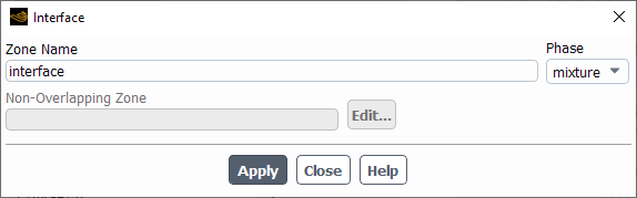
The Interface dialog box can be used to modify the name of an interface zone; there are no conditions to be set. It is opened from the Boundary Conditions Task Page. Interface zones are used for multiple reference frame and sliding mesh calculations, and for non-conformal meshes. See The Multiple Reference Frame Model, Setting Up the Sliding Mesh Problem, and Non-Conformal Meshes for details.
Controls
- Zone Name
sets the name of the zone.
- Non-Overlapping Zone
displays the name of the non-overlapping zone created for this interface zone as part of the creation of a mesh interface.
- Edit...
opens the boundary condition dialog box of the non-overlapping zone, so that you can easily review and/or revise the settings.
- Phase
displays the name of the phase. This item appears only for multiphase flows.
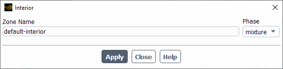
The Interior dialog box can be used to modify the name of an interior zone; there are no conditions to be set. It is opened from the Boundary Conditions Task Page.
Controls
- Zone Name
sets the name of the zone.
- Phase
displays the name of the phase. This item appears only for multiphase flows.
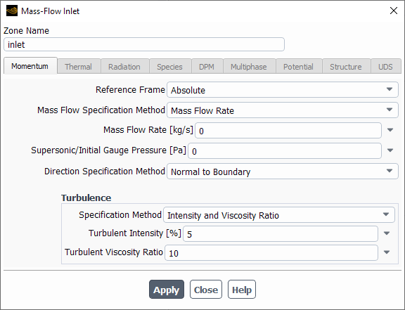
The Mass-Flow Inlet dialog box sets the boundary conditions for a mass-flow inlet zone. It is opened from the Boundary Conditions Task Page. See Inputs at Mass-Flow Inlet Boundaries for details about defining the items below.
Important: This feature offers reduced functionality when running Fluent under the Pro capability level.
Controls
- Zone Name
sets the name of the zone.
- Momentum
displays the momentum boundary conditions.
- Reference Frame
specifies the reference frame for the mass flow. If the cell zone adjacent to the mass-flow inlet is moving, you can choose to specify relative or absolute velocities by selecting Relative to Adjacent Cell Zone or Absolute in the Reference Frame drop-down list.
- Mass Flow Specification Method
specifies whether you are defining Mass Flow Rate, Mass Flux, or Mass Flux with Average Mass Flux.
- Mass Flow Rate
sets the prescribed mass flow rate for the zone. This flow rate is converted internally to a prescribed uniform mass flux over the zone by dividing the flow rate by the flow direction area projection of the zone. This item will appear if you selected Mass Flow Rate in the Mass Flow Specification Method list.
Important: Note that for axisymmetric problems, this mass flow rate is the flow rate through the entire (
 -radian) domain, not through a 1-radian slice.
- Mass Flux
sets the prescribed mass flux for the zone. This item will appear if you selected Mass Flux or Mass Flux with Average Mass Flux in the Mass Flow Specification Method list.
Important: Note that for axisymmetric problems, this mass flux is the flux through a 1-radian slice of the domain.
- Average Mass Flux
sets the average mass flux through the zone. See More About Mass Flux and Average Mass Flux for details. This item will appear if you selected Mass Flux with Average Mass Flux in the Mass Flow Specification Method list.
Important: Note that for axisymmetric problems, this mass flux is the flux through a 1-radian slice of the domain.
- Supersonic/Initialization Gauge Pressure
sets the static pressure that will be used to initialize the flow field if the mass-flow inlet boundary condition is selected for initializing flow properties (see Initializing the Entire Flow Field Using Standard Initialization).
- Direction Specification Method
specifies the method you will use to define the flow direction. If you choose Direction Vector, you will define the flow direction components, and if you choose Normal to Boundary no inputs are required. See Defining the Flow Direction for information on specifying flow direction.
- Coordinate System
specifies whether Cartesian, Cylindrical, Local Cylindrical,or Local Cylindrical Swirl vector components will be defined. This item will appear only for 3D cases in which you have selected Direction Vector as the Direction Specification Method.
- X-, Y-, Z-Component of Flow Direction
set the velocity-direction vector of the inflow stream. This vector does not need to be normalized (for example, you can specify the vector (1 1 1) rather than (0.577 0.577 0.577)). These items will appear if the selected Coordinate System is Cartesian or the model is 2D non-axisymmetric.
- Radial-, Tangential-, Axial-Component of Flow Direction
set the velocity-direction vector of the inflow stream. These items will appear for 2D axisymmetric cases, or for 3D cases for which the selected Coordinate System is Cylindrical or Local Cylindrical.
- Axial-, Radial-Component of Flow Direction, Tangential-Velocity
appear for a 3D Local Cylindrical Swirl coordinate system.
- Axis Origin
sets the X, Y, and Z coordinates of the origin of the local cylindrical (swirl) coordinate system.
- Axis Direction
sets the X, Y, and Z components of the direction of the local cylindrical (swirl) coordinate system.
- Turbulence
contains the turbulence parameters.
- Specification Method
specifies which method will be used to define the turbulence parameters. You can choose K and Epsilon (
 -
-  models and RSM only), K and Omega
(
models and RSM only), K and Omega
( -
-  models only), Intensity and Length Scale,
Intensity and Viscosity Ratio, Intensity and Hydraulic
Diameter, Modified Turbulent Viscosity (Spalart-Allmaras
model only), or Turbulent Viscosity Ratio (Spalart-Allmaras model
only). See Determining Turbulence Parameters for information about the inputs for each
of these methods. (This item will appear only for turbulent flow calculations.)
models only), Intensity and Length Scale,
Intensity and Viscosity Ratio, Intensity and Hydraulic
Diameter, Modified Turbulent Viscosity (Spalart-Allmaras
model only), or Turbulent Viscosity Ratio (Spalart-Allmaras model
only). See Determining Turbulence Parameters for information about the inputs for each
of these methods. (This item will appear only for turbulent flow calculations.)- Turbulent Kinetic Energy, Turbulent Dissipation Rate
set values for the turbulence kinetic energy
 and its dissipation rate
  . These items will appear if you choose K and
Epsilon as the Specification Method.
. These items will appear if you choose K and
Epsilon as the Specification Method.- Turbulent Kinetic Energy, Specific Dissipation Rate
set values for the turbulence kinetic energy
 and its specific dissipation rate
  . These items will appear if you choose K and
Omega as the Specification Method.
. These items will appear if you choose K and
Omega as the Specification Method.- Turbulent Intensity, Turbulent Length Scale
set values for turbulence intensity
 and turbulence length scale
  . These items will appear if you choose Intensity and Length
Scale as the Specification Method.
. These items will appear if you choose Intensity and Length
Scale as the Specification Method.- Turbulent Intensity, Turbulent Viscosity Ratio
set values for turbulence intensity
 and turbulent viscosity ratio
  . These items will appear if you choose Intensity and
Viscosity Ratio as the Specification Method.
. These items will appear if you choose Intensity and
Viscosity Ratio as the Specification Method.- Turbulent Intensity, Hydraulic Diameter
set values for turbulence intensity
 and hydraulic diameter
  . These items will appear if you choose Intensity and
Hydraulic Diameter as the Specification Method.
. These items will appear if you choose Intensity and
Hydraulic Diameter as the Specification Method.- Modified Turbulent Viscosity
sets the value of the modified turbulent viscosity
 . This item will appear if you choose Modified Turbulent
Viscosity as the Specification Method.
. This item will appear if you choose Modified Turbulent
Viscosity as the Specification Method.- Turbulent Viscosity Ratio
sets the value of the turbulent viscosity ratio
 . This item will appear if you choose Turbulent Viscosity
Ratio as the Specification Method.
. This item will appear if you choose Turbulent Viscosity
Ratio as the Specification Method.- Reynolds-Stress Specification Method
specifies which method will be used to determine the Reynolds stress boundary conditions when the Reynolds stress turbulence model is used. You can choose either K or Turbulent Intensity or Reynolds-Stress Components. If you choose the former, Ansys Fluent will compute the Reynolds stresses for you. If you choose the latter, you will explicitly specify the Reynolds stresses yourself. See Reynolds Stress Model for details. (This item will appear only for RSM turbulent flow calculations.)
- UU, VV, WW, UV, VW, UW Reynolds Stresses
specify the Reynolds stress components when Reynolds-Stress Components is chosen as the Reynolds-Stress Specification Method.
- Acoustic Wave Model
contains settings for treatment of acoustic pressure waves at the boundary.
- Off
disables special treatment of acoustic pressure waves at the boundary.
- Non Reflecting
enables the general non-reflecting boundary condition treatment described in General Non-Reflecting Boundary Conditions.
- Impedance
enables the impedance boundary condition treatment described in Impedance Boundary Conditions.
- Transparent Flow Forcing
enables the transparent flow forcing boundary condition described in Transparent Flow Forcing Boundary Conditions.
- Impedance Parameters
contains the parameters for the impedance boundary condition treatment. For details refer to Using the Impedance Boundary Condition.
- Transparent Flow Forcing Parameters
contains the parameters for the transparent flow forcing boundary condition treatment. For details refer to Using the Transparent Flow Forcing Boundary Condition.
- Thermal
contains the thermal parameters.
- Total Temperature
sets the total temperature of the inflow stream.
- Radiation
contains the radiation parameters.
- External Black Body Temperature Method, Internal Emissivity
set the radiation boundary conditions when you are using the P-1, DTRM, DO, S2S, or MC models for radiation heat transfer. See Defining Boundary Conditions for Radiation for details.
- Participates in Solar Ray Tracing
specifies whether or not the mass-flow inlet participates in solar ray tracing.
- Solar Transmissivity Factor
specifies a multiplier (ranging from 0 to 1) that is applied to the solar irradiation entering the domain through the mass-flow inlet.
- Participates in View Factor Calculation
specifies whether or not the mass-flow inlet participates in the view factor calculation as part of the S2S radiation model. This parameter is available only if you select the Surface to Surface radiation model.
- Species
contains the species parameters.
- Specify Species in Mole Fractions
allows you to specify the species in mole fractions rather than mass fractions.
- Species Mass Fractions
contains inputs for the mass fractions of defined species. See Defining Cell Zone and Boundary Conditions for Species for details about these inputs. These items will appear only if you are modeling non-reacting multi-species flow or you are using the finite-rate reaction formulation.
- Progress Variable
sets the value of the progress variable for premixed turbulent combustion. See Setting Boundary Conditions for the Progress Variable for details.
This item will appear only if the premixed or partially premixed combustion model is used.
- Mean Mixture Fraction, Mixture Fraction Variance
set inlet values for the PDF mixture fraction and its variance. (These items will appear only if you are using the non-premixed or partially premixed combustion model.)
- Secondary Mean Mixture Fraction, Secondary Mixture Fraction Variance
set inlet values for the secondary mixture fraction and its variance. (These items will appear only if you are using the non-premixed or partially premixed combustion model with two mixture fractions.)
- Scalar Mass Fractions
(partially-premixed combustion FGM model only) allows you to specify the scalar species mass fractions for the transported scalars that you selected in the Select Transported Scalars dialog box.
- DPM
contains the discrete phase parameters.
- Discrete Phase BC Type
sets the way that the discrete phase behaves with respect to the boundary. This item appears when one or more injections have been defined.
- reflect
rebounds the particle off the boundary with a change in its momentum as defined by the coefficient of restitution. (See Particle Reflection at Wall in the Fluent Theory Guide.)
- trap
terminates the trajectory calculations and records the fate of the particle as "trapped". In the case of evaporating droplets, their entire mass instantaneously passes into the vapor phase and enters the cell adjacent to the boundary. See Figure 24.40: “Trap” Boundary Condition for the Discrete Phase.
- escape
reports the particle as having "escaped" when it encounters the boundary. Trajectory calculations are terminated. See Figure 24.41: “Escape” Boundary Condition for the Discrete Phase.
- reinject
reintroduces the particle into the domain when it reaches a certain domain boundary (for example, outlet). This item appears when one or more injections have been defined and Unsteady Particle Tracking is enabled in the Discrete Phase Model dialog box. See The reinject Boundary Condition for details.
- wall-jet
indicates that the direction and velocity of the droplet particles are given by the resulting momentum flux, which is a function of the impingement angle. See Figure 12.6: "Wall Jet" Boundary Condition for the Discrete Phase in the Theory Guide.
- user-defined
specifies a user-defined function to define the discrete phase boundary condition type.
- Discrete Phase BC Function
sets the user-defined function from the drop-down list.
- Potential
displays the boundary conditions for the electric potential field. This tab is available only if you have enabled either the Electric Potential model or the Electrochemical reaction model in the Species Dialog Box.
- Potential Boundary Condition
is a drop-down list of available potential boundary condition types for the potential generated by electron current: Specified Flux and Specified Value. For the Specified Flux boundary condition, you will need to specify Current Density at the wall. For the Specified Value boundary condition, you will need to specify Potential at the wall.
- Electrolyte Potential Boundary Condition
is a drop-down list of available boundary condition types for the potential generated by ionic current. This item is similar to the Potential Boundary Condition drop-down list described above and is available only for the Electrolysis and H2 Pump model.
- UDS
contains the UDS parameters.
- User-Defined Scalar Boundary Condition
appears only if user-defined scalars are specified.
- User Scalar n
specifies whether the scalar is a specified flux or a specified value.
- User-Defined Scalar Boundary Value
appears only if user-defined scalars are specified.
- User Scalar n
specifies the value of the scalar.
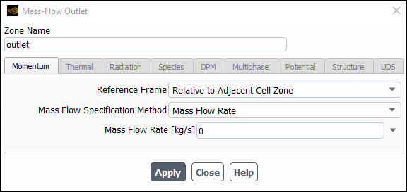
The Mass-Flow Outlet dialog box sets the boundary conditions for a mass-flow outlet zone. It is opened from the Boundary Conditions Task Page. See Inputs at Mass-Flow Outlet Boundaries for details about defining the items below.
Important: This feature offers reduced functionality when running Fluent under the Pro capability level.
Controls
- Zone Name
sets the name of the zone.
- Momentum
displays the momentum boundary conditions.
- Reference Frame
specifies the reference frame for the mass flow when the cell zone adjacent to the mass-flow outlet is moving. The only available option is Relative to Adjacent Cell Zone, so you must define the mass flow relative to the adjacent cell zone.
- Mass Flow Specification Method
specifies whether you are defining a Mass Flow Rate, Mass Flux, Mass Flux with Average Mass Flux, or (if the density of the material is defined either as an ideal gas or using a real gas model) Exit Corrected Mass Flow Rate.
- Mass Flow Rate
sets the prescribed mass flow rate for the zone. This flow rate is converted internally to a prescribed uniform mass flux over the zone by dividing the flow rate by the flow direction area projection of the zone. This item will appear if you selected Mass Flow Rate from the Mass Flow Specification Method drop-down list.
Important: Note that for axisymmetric problems, this mass flow rate is the flow rate through the entire (
 -radian) domain, not through a 1-radian slice.
- Mass Flux
sets the prescribed mass flux for the zone. This item will appear if you selected Mass Flux or Mass Flux with Average Mass Flux from the Mass Flow Specification Method drop-down list.
Important: Note that for axisymmetric problems, this mass flux is the flux through a 1-radian slice of the domain.
- Average Mass Flux
sets the average mass flux through the zone. For details, see Defining the Mass Flow Rate or Mass Flux. This item will appear if you selected Mass Flux with Average Mass Flux from the Mass Flow Specification Method drop-down list.
Important: Note that for axisymmetric problems, this mass flux is the flux through a 1-radian slice of the domain.
- Exit Corrected Mass Flow Rate
sets the value for an exit corrected mass flow rate that is maintained by adjusting the mass flow rate to the total conditions at the outlet. The resulting mass flow rate will be proportional to the exit total pressure and inversely proportional to the square root of the exit total temperature (or equivalently, inversely proportional to the stagnation speed of sound). For details, see Exit Corrected Mass Flow Rate. This item will appear if you selected Exit Corrected Mass Flow Rate from the Mass Flow Specification Method drop-down list.
Important: Note that for axisymmetric problems, this mass flow rate is the flow rate through the entire (
-radian) domain, not through a 1-radian slice.- ECMF Reference Temperature
sets the reference temperature for the exit corrected mass flow rate; for details, see Exit Corrected Mass Flow Rate. Typically, it is set to be the same as the inflow total temperature. This item will appear if you selected Exit Corrected Mass Flow Rate from the Mass Flow Specification Method drop-down list.
- ECMF Reference Gauge Pressure
sets the reference gauge pressure for the exit corrected mass flow rate; for details, see Exit Corrected Mass Flow Rate. Typically, it is set to be the same as the inflow total pressure. This item will appear if you selected Exit Corrected Mass Flow Rate from the Mass Flow Specification Method drop-down list.
- Coordinate System
specifies whether Cartesian, Cylindrical, Local Cylindrical,or Local Cylindrical Swirl vector components will be defined. This item will appear only for 3D cases in which you have selected Direction Vector as the Direction Specification Method.
- X-, Y-, Z-Component of Flow Direction
set the velocity-direction vector of the outflow stream. This vector does not need to be normalized (for example, you can specify the vector (1 1 1) rather than (0.577 0.577 0.577)). These items will appear if the selected Coordinate System is Cartesian or the model is 2D non-axisymmetric.
- Radial-, Tangential-, Axial-Component of Flow Direction
set the velocity-direction vector of the outflow stream. These items will appear for 2D axisymmetric cases, or for 3D cases for which the selected Coordinate System is Cylindrical or Local Cylindrical.
- Axial-, Radial-Component of Flow Direction, Tangential-Velocity
appear for a 3D Local Cylindrical Swirl coordinate system.
- Axis Origin
sets the X, Y, and Z coordinates of the origin of the local cylindrical (swirl) coordinate system.
- Axis Direction
sets the X, Y, and Z components of the direction of the local cylindrical (swirl) coordinate system.
- Radiation
contains the radiation parameters.
- External Black Body Temperature Method, Black Body Temperature, Internal Emissivity
set the radiation boundary conditions when you are using the P-1, DTRM, DO, S2S, or MC models for radiation heat transfer. See Defining Boundary Conditions for Radiation for details.
- Participates in Solar Ray Tracing
specifies whether or not the mass-flow outlet participates in solar ray tracing.
- Solar Transmissivity Factor
specifies a multiplier (ranging from 0 to 1) that is applied to the solar irradiation entering the domain through the mass-flow outlet.
- Participates in View Factor Calculation
specifies whether or not the mass-flow outlet participates in the view factor calculation as part of the S2S radiation model. This parameter is available only if you select the Surface to Surface radiation model.
- DPM
contains the discrete phase parameters.
- Discrete Phase BC Type
sets the way that the discrete phase behaves with respect to the boundary. This item appears when one or more injections have been defined.
- reflect
rebounds the particle off the boundary with a change in its momentum as defined by the coefficient of restitution. (See Particle Reflection at Wall in the Fluent Theory Guide.)
- trap
terminates the trajectory calculations and records the fate of the particle as "trapped". In the case of evaporating droplets, their entire mass instantaneously passes into the vapor phase and enters the cell adjacent to the boundary. See Figure 24.40: “Trap” Boundary Condition for the Discrete Phase.
- escape
reports the particle as having "escaped" when it encounters the boundary. Trajectory calculations are terminated. See Figure 24.41: “Escape” Boundary Condition for the Discrete Phase.
- reinject
reintroduces the particle into the domain when it reaches a certain domain boundary (for example, outlet). This item appears when one or more injections have been defined and Unsteady Particle Tracking is enabled in the Discrete Phase Model dialog box. See The reinject Boundary Condition for details.
- wall-jet
indicates that the direction and velocity of the droplet particles are given by the resulting momentum flux, which is a function of the impingement angle. See Figure 12.6: "Wall Jet" Boundary Condition for the Discrete Phase in the Theory Guide.
- user-defined
specifies a user-defined function to define the discrete phase boundary condition type.
- Discrete Phase BC Function
sets the user-defined function from the drop-down list.
- UDS
contains the UDS parameters.
- User-Defined Scalar Boundary Condition
appears only if user-defined scalars are specified.
- User Scalar n
specifies whether the scalar is a specified flux or a specified value.
- User-Defined Scalar Boundary Value
appears only if user-defined scalars are specified.
- User Scalar n
specifies the value of the scalar.
The Outflow dialog box sets the boundary conditions for an outflow zone. It is opened from the Boundary Conditions Task Page. See Using Outflow Boundaries for details about using outflow boundaries.
Important: This feature offers reduced functionality when running Fluent under the Pro capability level.
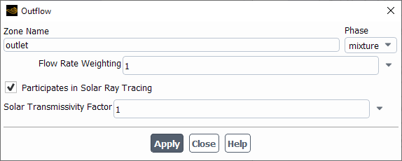
Controls
- Zone Name
sets the name of the zone.
- Flow Rate Weighting
specifies the portion of the outflow that is going through the boundary. See Mass Flow Split Boundary Conditions for details.
- External Black Body Temperature Method, Internal Emissivity
set the radiation boundary conditions when you are using the P-1, DTRM, DO, S2S, or MC models for radiation heat transfer. See Defining Boundary Conditions for Radiation for details.
- Discrete Phase BC Type
sets the way that the discrete phase behaves with respect to the boundary. This item appears when one or more injections have been defined.
- reflect
rebounds the particle off the boundary with a change in its momentum as defined by the coefficient of restitution. (See Particle Reflection at Wall in the Fluent Theory Guide.)
- trap
terminates the trajectory calculations and records the fate of the particle as "trapped". In the case of evaporating droplets, their entire mass instantaneously passes into the vapor phase and enters the cell adjacent to the boundary. See Figure 24.40: “Trap” Boundary Condition for the Discrete Phase.
- escape
reports the particle as having "escaped" when it encounters the boundary. Trajectory calculations are terminated. See Figure 24.41: “Escape” Boundary Condition for the Discrete Phase.
- reinject
reintroduces the particle into the domain when it reaches a certain domain boundary (for example, outlet). This item appears when one or more injections have been defined and Unsteady Particle Tracking is enabled in the Discrete Phase Model dialog box. See The reinject Boundary Condition for details.
- wall-jet
indicates that the direction and velocity of the droplet particles are given by the resulting momentum flux, which is a function of the impingement angle. See Figure 12.6: "Wall Jet" Boundary Condition for the Discrete Phase in the Theory Guide.
- user-defined
specifies a user-defined function to define the discrete phase boundary condition type.
- Participates in Solar Ray Tracing
specifies whether or not outflow participate in solar ray tracing.
- Solar Transmissivity Factor
specifies a multiplier (ranging from 0 to 1) that is applied to the solar irradiation entering the domain through the outflow.
- Discrete Phase BC Function
sets the user-defined function from the drop-down list.
- Participates in View Factor Calculation
specifies whether or not the outflow participates in the view factor calculation as part of the S2S radiation model. This parameter is available only if you select the Surface to Surface radiation model.
The Outlet Vent dialog box sets the boundary conditions for an outlet vent zone. It is opened from the Boundary Conditions Task Page. See Inputs at Outlet Vent Boundaries for details about defining the items below.
Important: This feature offers reduced functionality when running Fluent under the Pro capability level..
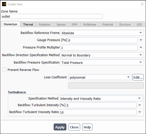
Controls
- Zone Name
sets the name of the zone.
- Momentum
contains the momentum parameters.
- Backflow Reference Frame
specify whether backflow temperature, pressure, and flow directions are in the Absolute or Relative to the Adjacent Cell Zone reference frame.
- Gauge Pressure
sets the gauge pressure at the outlet boundary.
- Backflow Direction Specification Method
specifies the method you will use to define the flow direction. If you choose Direction Vector, you will define the flow direction components, and if you choose Normal to Boundary or From Neighboring Cell no inputs are required. See Defining the Flow Direction for information on specifying flow direction.
- Coordinate System
contains a drop-down list for selecting the coordinate system. You can choose Cartesian, Cylindrical, or Local Cylindrical. This option is available only when Direction Vector is selected from the Backflow Direction Specification Method drop-down list.
- X-, Y-, Z-Component of Flow Direction
allows you to specify the velocity components in x, y, and z directions respectively. This option is available when Cartesian is selected for the Coordinate System.
- Radial-, Tangential-, Axial-Component of Flow Direction
set the direction of the flow at the boundary. These items will appear for 2D axisymmetric cases, or for 3D cases for which the selected Coordinate System is Cylindrical or Local Cylindrical.
- Backflow Pressure Specification
specifies how the pressure is calculated under backflow conditions. If you select Static Pressure, the Gauge Pressure is directly imposed as the boundary face pressure; if you select Total Pressure, the Gauge Pressure will be combined with a dynamic contribution that is based on the velocity in the adjacent cell zone.
- Loss-Coefficient
sets the non-dimensional loss coefficient used to compute the pressure drop. See Specifying the Loss Coefficient for details.
- Axis Origin
sets the X, Y, and Z coordinates of the origin of the local cylindrical coordinate system.
- Axis Direction
sets the X, Y, and Z components of the direction of the local cylindrical coordinate system.
- Turbulence
contains the turbulence parameters.
- Specification Method
specifies which method will be used to define the turbulence parameters. You can choose K and Epsilon (
 -
-  models and RSM only), K and Omega
(
models and RSM only), K and Omega
( -
-  models only), Intensity and Length Scale,
Intensity and Viscosity Ratio, Intensity and Hydraulic
Diameter, Modified Turbulent Viscosity (Spalart-Allmaras
model only), or Turbulent Viscosity Ratio (Spalart-Allmaras model
only). See Determining Turbulence Parameters for information about the inputs for each
of these methods. (This item will appear only for turbulent flow calculations.)
models only), Intensity and Length Scale,
Intensity and Viscosity Ratio, Intensity and Hydraulic
Diameter, Modified Turbulent Viscosity (Spalart-Allmaras
model only), or Turbulent Viscosity Ratio (Spalart-Allmaras model
only). See Determining Turbulence Parameters for information about the inputs for each
of these methods. (This item will appear only for turbulent flow calculations.)- Backflow Turbulent Kinetic Energy, Backflow Turbulent Dissipation Rate
set values for the turbulence kinetic energy
 and its dissipation rate
  . These items will appear if you choose K and
Epsilon as the Specification Method.
. These items will appear if you choose K and
Epsilon as the Specification Method.- Backflow Turbulent Kinetic Energy, Backflow Specific Dissipation Rate
set values for the turbulence kinetic energy
 and its specific dissipation rate
  . These items will appear if you choose K and
Omega as the Specification Method.
. These items will appear if you choose K and
Omega as the Specification Method.- Backflow Turbulent Intensity, Backflow Turbulent Length Scale
set values for turbulence intensity
 and turbulence length scale
  . These items will appear if you choose Intensity and Length
Scale as the Specification Method.
. These items will appear if you choose Intensity and Length
Scale as the Specification Method.- Backflow Turbulent Intensity, Backflow Turbulent Viscosity Ratio
set values for turbulence intensity
 and turbulent viscosity ratio
  . These items will appear if you choose Intensity and
Viscosity Ratio as the Specification Method.
. These items will appear if you choose Intensity and
Viscosity Ratio as the Specification Method.- Backflow Turbulent Intensity, Backflow Hydraulic Diameter
set values for turbulence intensity
 and hydraulic diameter
  . These items will appear if you choose Intensity and
Hydraulic Diameter as the Specification Method.
. These items will appear if you choose Intensity and
Hydraulic Diameter as the Specification Method.- Backflow Modified Turbulent Viscosity
sets the value of the backflow modified turbulent viscosity
 . This item will appear if you choose Modified Turbulent
Viscosity as the Specification Method.
. This item will appear if you choose Modified Turbulent
Viscosity as the Specification Method.- Backflow Turbulent Viscosity Ratio
sets the value of the backflow turbulent viscosity ratio
 . This item will appear if you choose Turbulent Viscosity
Ratio as the Specification Method.
. This item will appear if you choose Turbulent Viscosity
Ratio as the Specification Method.- Reynolds-Stress Specification Method
specifies which method will be used to determine the backflow Reynolds stress boundary conditions when the Reynolds stress turbulence model is used. You can choose either K or Turbulent Intensity or Reynolds-Stress Components. If you choose the former, Ansys Fluent will compute the Reynolds stresses for you. If you choose the latter, you will explicitly specify the Reynolds stresses yourself. See Reynolds Stress Model for details. (This item will appear only for RSM turbulent flow calculations.)
- Backflow UU, VV, WW, UV, VW, UW Reynolds Stresses
specify the backflow Reynolds stress components when Reynolds-Stress Components is chosen as the Reynolds-Stress Specification Method.
- Thermal
contains the thermal parameters.
- Backflow Total Temperature
sets the total temperature of the inflow stream should the flow reverse direction
- Radiation
contains the boundary conditions for the radiation model at the outlet vent.
- External Black Body Temperature Method, Internal Emissivity
set the radiation boundary conditions when you are using the P-1, DTRM, DO, S2S, or MC models for radiation heat transfer. See Defining Boundary Conditions for Radiation for details.
- Participates in Solar Ray Tracing
specifies whether or not the outlet vent participates in solar ray tracing.
- Solar Transmissivity Factor
specifies a multiplier (ranging from 0 to 1) that is applied to the solar irradiation entering the domain through the outlet vent.
- Participates in View Factor Calculation
specifies whether or not the outlet vent participates in the view factor calculation as part of the S2S radiation model. This parameter is available only if you select the Surface to Surface radiation model.
- Species
contains the species parameters.
- Specify Species in Mole Fractions
allows you to specify the species in mole fractions rather than mass fractions.
- Mean Mixture Fraction, Mixture Fraction Variance
set inlet values for the PDF mixture fraction and its variance. (These items will appear only if you are using the non-premixed or partially premixed combustion model.)
- Secondary Mean Mixture Fraction, Secondary Mixture Fraction Variance
set inlet values for the secondary mixture fraction and its variance. (These items will appear only if you are using the non-premixed or partially premixed combustion model with two mixture fractions.)
- Species Mass Fractions
contains inputs for the mass fractions of defined species. See Defining Cell Zone and Boundary Conditions for Species for details about these inputs. These items will appear only if you are modeling non-reacting multi-species flow or you are using the finite-rate reaction formulation.
- Backflow Progress Variable
sets the value of the progress variable for premixed turbulent combustion. See Setting Boundary Conditions for the Progress Variable for details.
This item will appear only if the premixed or partially premixed combustion model is used.
- DPM
contains the discrete phase parameters.
- Discrete Phase BC Type
sets the way that the discrete phase behaves with respect to the boundary. This item appears when one or more injections have been defined.
- reflect
rebounds the particle off the boundary with a change in its momentum as defined by the coefficient of restitution. (See Particle Reflection at Wall in the Fluent Theory Guide.)
- trap
terminates the trajectory calculations and records the fate of the particle as "trapped". In the case of evaporating droplets, their entire mass instantaneously passes into the vapor phase and enters the cell adjacent to the boundary. See Figure 24.40: “Trap” Boundary Condition for the Discrete Phase.
- escape
reports the particle as having "escaped" when it encounters the boundary. Trajectory calculations are terminated. See Figure 24.41: “Escape” Boundary Condition for the Discrete Phase.
- reinject
reintroduces the particle into the domain when it reaches a certain domain boundary (for example, outlet). This item appears when one or more injections have been defined and Unsteady Particle Tracking is enabled in the Discrete Phase Model dialog box. See The reinject Boundary Condition for details.
- wall-jet
indicates that the direction and velocity of the droplet particles are given by the resulting momentum flux, which is a function of the impingement angle. See Figure 12.6: "Wall Jet" Boundary Condition for the Discrete Phase in the Theory Guide.
- user-defined
specifies a user-defined function to define the discrete phase boundary condition type.
- Discrete Phase BC Function
sets the user-defined function from the drop-down list.
- Multiphase
contains the multiphase parameters.
- Backflow Granular Temperature
specifies temperature for the solids phase and is proportional to the kinetic energy of the random motion of the particles.
- Volume Fraction Specification Method
sets the method used to specify the volume fraction of the secondary phase selected in the Boundary Conditions Task Page. This section of the dialog box will appear when one of the multiphase models is being used. See Defining Multiphase Cell Zone and Boundary Conditions for details.
- Backflow Volume Fraction
specifies the volume fraction of the secondary phase as a constant, profile, of UDF function.
- From Neighboring Cell
calculates the volume fraction from the neighboring cells.
- Potential
displays the boundary conditions for the electric potential field. This tab is available only if you have enabled either the Electric Potential model or the Electrochemical reaction model in the Species Dialog Box.
- Potential Boundary Condition
is a drop-down list of available potential boundary condition types for the potential generated by electron current: Specified Flux and Specified Value. For the Specified Flux boundary condition, you will need to specify Current Density at the wall. For the Specified Value boundary condition, you will need to specify Potential at the wall.
- Electrolyte Potential Boundary Condition
is a drop-down list of available boundary condition types for the potential generated by ionic current. This item is similar to the Potential Boundary Condition drop-down list described above and is available only for the Electrolysis and H2 Pump model.
- UDS
contains the UDS parameters.
- User-Defined Scalar Boundary Condition
appears only if user-defined scalars are specified.
- User Scalar n
specifies whether the scalar is a specified flux or a specified value.
- User-Defined Scalar Boundary Value
appears only if user-defined scalars are specified.
- User Scalar n
specifies the value of the scalar.
The Overset dialog box sets the boundary conditions for an overset zone. It is opened from the Boundary Conditions Task Page. See Setting up an Overset Interface for further details.
Controls
- Zone Name
sets the name of the zone.
The Periodic dialog box sets the boundary conditions for a periodic zone. It is opened from the Boundary Conditions Task Page. See Inputs for Periodic Boundaries for details about the items below. See Periodic Flows for information about fully-developed periodic flow.
Controls
- Zone Name
sets the name of the zone.
- Periodic Type
indicates whether the periodicity of the domain is Translational or Rotational.
- Periodic Pressure Jump
sets the pressure increase/decrease across the periodic boundary. (This item will not appear if the pressure-based (default) solver is used; it is relevant only for the density-based solvers.)
The Porous Jump dialog box sets the boundary conditions for a porous-jump zone. It is opened from the Boundary Conditions Task Page. See Porous Jump Boundary Conditions for details about the items below.
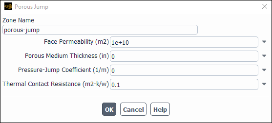
Controls
- Zone Name
sets the name of the zone.
- Face Permeability
sets the face permeability coefficient (
 in Equation 7–152).
- Porous Medium Thickness
sets the thickness of the porous medium (
 ).
).- Pressure-Jump Coefficient
sets the pressure-jump coefficient (
 ).
).- Thermal Contact Resistance
sets the thermal contact resistance.
- Jump Adhesion
sets the adhesion method and contact angle.
- Constrained-Two-Sided Adhesion
constrains the contact angle at the porous jump, When this option is disabled then the forced two-sided adhesion treatment is in effect. See Jump Adhesion for more information.
- Contact Angle
is the contact angle at the porous jump.
- Discrete Phase BC Type
sets the way that the discrete phase behaves with respect to the boundary. This item appears when one or more injections have been defined.
- interior
allows the particles to pass through the boundary.
- reflect
rebounds the particle off the boundary with a change in its momentum as defined by the coefficient of restitution. (See Particle Reflection at Wall in the Fluent Theory Guide.)
- trap
terminates the trajectory calculations and records the fate of the particle as "trapped". In the case of evaporating droplets, their entire mass instantaneously passes into the vapor phase and enters the cell adjacent to the boundary. See Figure 24.40: “Trap” Boundary Condition for the Discrete Phase.
- escape
reports the particle as having "escaped" when it encounters the boundary. Trajectory calculations are terminated. See Figure 24.41: “Escape” Boundary Condition for the Discrete Phase.
- reinject
reintroduces the particle into the domain when it reaches a certain domain boundary (for example, outlet). This item appears when one or more injections have been defined and Unsteady Particle Tracking is enabled in the Discrete Phase Model dialog box. See The reinject Boundary Condition for details.
- wall-jet
indicates that the direction and velocity of the droplet particles are given by the resulting momentum flux, which is a function of the impingement angle. See Figure 12.6: "Wall Jet" Boundary Condition for the Discrete Phase in the Theory Guide.
- user-defined
specifies a user-defined function to define the discrete phase boundary condition type.
- Discrete Phase BC Function
sets the user-defined function from the drop-down list.
- Solar Boundary Conditions
contains the settings for solar ray tracing. This group box is available only if you select Solar Ray Tracing from the Model list in the Solar Load group box of the Radiation Model dialog box. See Solar Ray Tracing for details.
- Participates in Solar Ray Tracing
specifies whether or not the porous jump participates in solar ray tracing.
- Absorptivity
contains the settings that define the absorptivity of the porous jump.
- Direct Visible
specifies a multiplier (ranging from 0 to 1) that is applied to the visible portion of the direct solar radiation spectrum to account for the absorption of the porous jump.
- Direct IR
specifies a multiplier (ranging from 0 to 1) that is applied to the infrared portion of the direct solar radiation spectrum to account for the absorption of the porous jump.
- Transmissivity
contains the settings that define the transmissivity of the porous jump.
- Direct Visible
specifies a multiplier (ranging from 0 to 1) that is applied to the visible portion of the direct solar radiation spectrum to account for the transmissivity of the porous jump.
- Direct IR
specifies a multiplier (ranging from 0 to 1) that is applied to the infrared portion of the direct solar radiation spectrum to account for the transmissivity of the porous jump.
The Pressure Far-Field dialog box sets the boundary conditions for a pressure far-field zone. It is opened from the Boundary Conditions Task Page. See Inputs at Pressure Far-Field Boundaries for details about defining the items below.
Important: This feature offers reduced functionality when running Fluent under the Pro capability level.
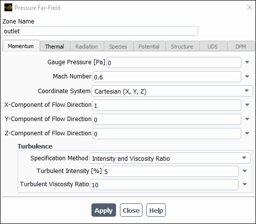
Controls
- Zone Name
sets the name of the zone.
- Momentum
contains the momentum parameters.
- Gauge Pressure
sets the far-field gauge static pressure.
- Mach Number
sets the far-field Mach number. The Mach number can be subsonic, sonic, or supersonic.
- Coordinate System
allows you to select a Cartesian, Cylindrical, or Local Cylindrical coordinate system. This option is available only for 3D geometry.
- X-, Y-, Z-Component of Flow Direction
set the far-field flow direction. These items will appear if the selected Coordinate System is Cartesian or the model is 2D non-axisymmetric.
- Radial-, Tangential-, Axial-Component of Flow Direction
set the far-field flow direction. These items will appear for 2D axisymmetric cases, or for 3D cases for which the selected Coordinate System is Cylindrical or Local Cylindrical.
- Axis Origin
sets the X, Y, and Z coordinates of the origin of the local cylindrical coordinate system.
- Axis Direction
sets the X, Y, and Z components of the direction of the local cylindrical coordinate system.
- Turbulence
contains the turbulence parameters.
- Specification Method
specifies which method will be used to define the turbulence parameters. You can choose K and Epsilon (
 -
-  models and RSM only), K and Omega
(
models and RSM only), K and Omega
( -
-  models only), Intensity and Length Scale,
Intensity and Viscosity Ratio, Intensity and Hydraulic
Diameter, Modified Turbulent Viscosity (Spalart-Allmaras
model only), or Turbulent Viscosity Ratio (Spalart-Allmaras model
only). See Determining Turbulence Parameters for information about the inputs for each
of these methods. (This item will appear only for turbulent flow calculations.)
models only), Intensity and Length Scale,
Intensity and Viscosity Ratio, Intensity and Hydraulic
Diameter, Modified Turbulent Viscosity (Spalart-Allmaras
model only), or Turbulent Viscosity Ratio (Spalart-Allmaras model
only). See Determining Turbulence Parameters for information about the inputs for each
of these methods. (This item will appear only for turbulent flow calculations.)- Turbulent Kinetic Energy, Turbulent Dissipation Rate
set values for the turbulence kinetic energy
 and its dissipation rate
  . These items will appear if you choose K and
Epsilon as the Specification Method.
. These items will appear if you choose K and
Epsilon as the Specification Method.- Turbulent Kinetic Energy, Specific Dissipation Rate
set values for the turbulence kinetic energy
 and its specific dissipation rate
  . These items will appear if you choose K and
Omega as the Specification Method.
. These items will appear if you choose K and
Omega as the Specification Method.- Turbulent Intensity, Turbulent Length Scale
set values for turbulence intensity
 and turbulence length scale
  . These items will appear if you choose Intensity and Length
Scale as the Specification Method.
. These items will appear if you choose Intensity and Length
Scale as the Specification Method.- Turbulent Intensity, Turbulent Viscosity Ratio
set values for turbulence intensity
 and turbulent viscosity ratio
  . These items will appear if you choose Intensity and
Viscosity Ratio as the Specification Method.
. These items will appear if you choose Intensity and
Viscosity Ratio as the Specification Method.- Turbulent Intensity, Hydraulic Diameter
set values for turbulence intensity
 and hydraulic diameter
  . These items will appear if you choose Intensity and
Hydraulic Diameter as the Specification Method.
. These items will appear if you choose Intensity and
Hydraulic Diameter as the Specification Method.- Modified Turbulent Viscosity
sets the value of the modified turbulent viscosity
 . This item will appear if you choose Modified Turbulent
Viscosity as the Specification Method.
. This item will appear if you choose Modified Turbulent
Viscosity as the Specification Method.- Turbulent Viscosity Ratio
sets the value of the turbulent viscosity ratio
 . This item will appear if you choose Turbulent Viscosity
Ratio as the Turbulence Specification Method.
. This item will appear if you choose Turbulent Viscosity
Ratio as the Turbulence Specification Method.- Reynolds-Stress Specification Method
specifies which method will be used to determine the Reynolds stress boundary conditions when the Reynolds stress turbulence model is used. You can choose either K or Turbulent Intensity or Reynolds-Stress Components. If you choose the former, Ansys Fluent will compute the Reynolds stresses for you. If you choose the latter, you will explicitly specify the Reynolds stresses yourself. See Reynolds Stress Model for details. (This item will appear only for RSM turbulent flow calculations.)
- UU, VV, WW, UV, VW, UW Reynolds Stresses
specify the Reynolds stress components when Reynolds-Stress Components is chosen as the Reynolds-Stress Specification Method.
- Thermal
contains the thermal parameters.
- Temperature
sets the far-field static temperature.
- Radiation
contains the boundary conditions for the radiation model at the pressure far-field zone.
- External Black Body Temperature Method, Internal Emissivity
set the radiation boundary conditions when you are using the P-1, DTRM, DO, S2S, or MC models for radiation heat transfer. See Defining Boundary Conditions for Radiation for details.
- Participates in Solar Ray Tracing
specifies whether or not the pressure far-field zone participates in solar ray tracing.
- Solar Transmissivity Factor
specifies a multiplier (ranging from 0 to 1) that is applied to the solar irradiation entering the domain through the pressure far-field zone.
- Participates in View Factor Calculation
specifies whether or not the pressure far-field zone participates in the view factor calculation as part of the S2S radiation model. This parameter is available only if you select the Surface to Surface radiation model.
- Species
contains the species parameters.
- Specify Species in Mole Fractions
allows you to specify the species in mole fractions rather than mass fractions.
- Species Mass Fractions
contains inputs for the mass fractions of defined species. See Defining Cell Zone and Boundary Conditions for Species for details about these inputs. (These items will appear only if you are modeling non-reacting multi-species flow or you are using the finite-rate reaction formulation.)
- Mean Mixture Fraction, Mixture Fraction Variance
set inlet values for the PDF mixture fraction and its variance. (These items will appear only if you are using the non-premixed or partially premixed combustion model.)
- Secondary Mean Mixture Fraction, Secondary Mixture Fraction Variance
set inlet values for the secondary mixture fraction and its variance. (These items will appear only if you are using the non-premixed or partially premixed combustion model with two mixture fractions.)
- Progress Variable
sets the value of the progress variable for premixed turbulent combustion. See Setting Boundary Conditions for the Progress Variable for details.
This item will appear only if the premixed or partially premixed combustion model is used.
- UDS
contains the UDS parameters.
- User-Defined Scalar Boundary Condition
appears only if user-defined scalars are specified.
- User Scalar n
specifies whether the scalar is a specified flux or a specified value.
- User-Defined Scalar Boundary Value
appears only if user-defined scalars are specified.
- User Scalar n
specifies the value of the scalar.
- DPM
contains the discrete phase parameters.
- Discrete Phase BC Type
sets the way that the discrete phase behaves with respect to the boundary. This item appears when one or more injections have been defined.
- reflect
rebounds the particle off the boundary with a change in its momentum as defined by the coefficient of restitution. (See Particle Reflection at Wall in the Fluent Theory Guide.)
- trap
terminates the trajectory calculations and records the fate of the particle as "trapped". In the case of evaporating droplets, their entire mass instantaneously passes into the vapor phase and enters the cell adjacent to the boundary. See Figure 24.40: “Trap” Boundary Condition for the Discrete Phase.
- escape
reports the particle as having "escaped" when it encounters the boundary. Trajectory calculations are terminated. See Figure 24.41: “Escape” Boundary Condition for the Discrete Phase.
- reinject
reintroduces the particle into the domain when it reaches a certain domain boundary (for example, outlet). This item appears when one or more injections have been defined and Unsteady Particle Tracking is enabled in the Discrete Phase Model dialog box. See The reinject Boundary Condition for details.
- wall-jet
indicates that the direction and velocity of the droplet particles are given by the resulting momentum flux, which is a function of the impingement angle. See Figure 12.6: "Wall Jet" Boundary Condition for the Discrete Phase in the Theory Guide.
- user-defined
specifies a user-defined function to define the discrete phase boundary condition type.
- Discrete Phase BC Function
sets the user-defined function from the drop-down list.
The Pressure Inlet dialog box sets the boundary conditions for a pressure inlet zone. It is opened from the Boundary Conditions Task Page. See Inputs at Pressure Inlet Boundaries for details about defining the items below.
Important: This feature offers reduced functionality when running Fluent under the Pro capability level.
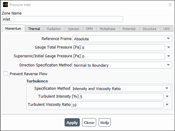
Controls
- Zone Name
sets the name of the zone.
- Momentum
contains the momentum parameters.
- Reference Frame
specifies the reference frame for the pressure inlet. If the cell zone adjacent to the pressure inlet is moving, you can choose to specify the total temperature, total pressure, and velocity components as Relative to Adjacent CellZone or Absolute in the Reference Frame drop-down list.
- Gauge Total Pressure
sets the gauge total (or stagnation) pressure of the inflow stream. If you are using moving reference frames, see Defining Total Pressure and Temperature for information about relative and absolute total pressure.
- Supersonic/Initial Gauge Pressure
sets the static pressure on the boundary when the flow becomes (locally) supersonic. It is also used to compute initial values for pressure, temperature, and velocity if the pressure inlet boundary condition is selected for computing initial values (see Initializing the Entire Flow Field Using Standard Initialization).
- Direction Specification Method
specifies the method you will use to define the flow direction. If you choose Direction Vector, you will define the flow direction components, and if you choose Normal to Boundary no inputs are required. You also have the option to enable Prevent Reverse Flow. See Defining the Flow Direction for information on specifying flow direction.
- Coordinate System
specifies whether Cartesian, Cylindrical, Local Cylindrical,or Local Cylindrical Swirl vector components will be defined. This item will appear only for 3D cases in which you have selected Direction Vector as the Direction Specification Method.
- X,Y,Z-Component of Flow Direction
set the direction of the flow at the inlet boundary. These items will appear if the selected Coordinate System is Cartesian or the model is 2D non-axisymmetric.
- Radial, Tangential, Axial Component of Flow Direction
set the direction of the flow at the inlet boundary. These items will appear for 2D axisymmetric cases, or for 3D cases for which the selected Coordinate System is Cylindrical or Local Cylindrical.
- Radial-, Axial-Component of Flow Direction, Tangential-Velocity
appear for a 3D Local Cylindrical Swirl coordinate system.
- Axis Origin
sets the X, Y, and Z coordinates of the origin of the local cylindrical (swirl) coordinate system.
- Axis Direction
sets the X, Y, and Z components of the direction of the local cylindrical (swirl) coordinate system.
- Prevent Reverse Flow
Enables Fluent to erect artificial walls on the boundary mesh faces to prevent flow out of the domain. The artificial walls are removed when the flow is no longer leaving the domain and when a favorable pressure gradient is recovered at the boundary mesh faces.
- Fluctuating Velocity
contains parameters for Inlet Boundary Conditions for Scale Resolving Simulations (only available for transient cases where scale-resolving turbulence models such as SAS, DES, and LES are enabled).
- Fluctuating Velocity Algorithm
Specifies which method will be used for generating fluctuations at the boundary for Scale Resolving Simulations. The following methods are available:
- No Perturbations
No fluctuations added.
- Vortex Method
For details, see Vortex Method in the Fluent Theory Guide.
- Spectral Synthesizer
For details, see Spectral Synthesizer in the Fluent Theory Guide.
- Synthetic Turbulence Generator
For details, see Synthetic Turbulence Generator in the Fluent Theory Guide.
- Number of Vortices
Specifies number of vortices to be generated with the Vortex Method.
- Satisfy Mass Conservation?
Enables mass conservation for the Vortex Method at the boundary.
- Scale Search Limiter
Specifies which method will be used to limit the area from where global scales for the Synthetic Turbulence Generator are computed. The following methods are available:
- None
Scales are computed using the entire inlet zone.
- Turbulent Intensity Threshold
Scales are computed using only part of the inlet zone where Turbulent Intensity is higher than specified threshold value.
- Turbulent Viscosity Ratio Threshold
Scales are computed using only part of the inlet zone where Turbulent Viscosity Ratio is higher than specified threshold value.
- Wall Distance Threshold
Scales are computed using only part of the inlet zone where Wall Distance is smaller than specified threshold value.
- Turbulent Intensity, Turbulent Viscosity Ratio, or Wall Distance
Specifies threshold value for the corresponding Scale Search Limiter (only available for the Synthetic Turbulence Generator with corresponding Scale Search Limiter chosen).
- Volumetric Forcing?
Enables generation of fluctuations in the volume adjacent to the inlet boundary instead of introduction of fluctuations directly at the boundary (only available for the Synthetic Turbulence Generator).
- Forcing Zone Thickness
Specifies which method will be used to set up the streamwise size of the volume where fluctuations are to be generated (only available for the Synthetic Turbulence Generator with Volumetric Forcing? enabled). The following methods are available:
- Automatic
Length is computed based on the turbulent length scale computed from the boundary.
- Specified Value
Length is specified by the user.
- Thickness
Specifies the streamwise size of the volume where fluctuations are to be generated (only available for the Synthetic Turbulence Generator with Volumetric Forcing? enabled if Specified Value option is chosen for Forcing Zone Thickness).
- Turbulence
contains the turbulence parameters.
- Specification Method
specifies which method will be used to define the turbulence parameters. You can choose K and Epsilon (
 -
-  models and RSM only), K and Omega
(
models and RSM only), K and Omega
( -
-  models only), Intensity and Length Scale,
Intensity and Viscosity Ratio, Intensity and Hydraulic
Diameter, Modified Turbulent Viscosity (Spalart-Allmaras
model only), or Turbulent Viscosity Ratio (Spalart-Allmaras model
only). See Determining Turbulence Parameters for information about the inputs for each
of these methods. (This item will appear only for turbulent flow calculations.)
models only), Intensity and Length Scale,
Intensity and Viscosity Ratio, Intensity and Hydraulic
Diameter, Modified Turbulent Viscosity (Spalart-Allmaras
model only), or Turbulent Viscosity Ratio (Spalart-Allmaras model
only). See Determining Turbulence Parameters for information about the inputs for each
of these methods. (This item will appear only for turbulent flow calculations.)- Turbulent Kinetic Energy, Turbulent Dissipation Rate
set values for the turbulence kinetic energy
 and its dissipation rate
  . These items will appear if you choose K and
Epsilon as the Specification Method.
. These items will appear if you choose K and
Epsilon as the Specification Method.- Turbulent Kinetic Energy, Specific Dissipation Rate
set values for the turbulence kinetic energy
 and its specific dissipation rate
  . These items will appear if you choose K and
Omega as the Specification Method.
. These items will appear if you choose K and
Omega as the Specification Method.- Turbulent Intensity, Turbulent Length Scale
set values for turbulence intensity
 and turbulence length scale
  . These items will appear if you choose Intensity and Length
Scale as the Specification Method.
. These items will appear if you choose Intensity and Length
Scale as the Specification Method.- Turbulent Intensity, Turbulent Viscosity Ratio
set values for turbulence intensity
 and turbulent viscosity ratio
  . These items will appear if you choose Intensity and
Viscosity Ratio as the Specification Method.
. These items will appear if you choose Intensity and
Viscosity Ratio as the Specification Method.- Turbulent Intensity, Hydraulic Diameter
set values for turbulence intensity
 and hydraulic diameter
  . These items will appear if you choose Intensity and
Hydraulic Diameter as the Specification Method.
. These items will appear if you choose Intensity and
Hydraulic Diameter as the Specification Method.- Modified Turbulent Viscosity
sets the value of the modified turbulent viscosity
 . This item will appear if you choose Modified Turbulent
Viscosity as the Specification Method.
. This item will appear if you choose Modified Turbulent
Viscosity as the Specification Method.- Turbulent Viscosity Ratio
sets the value of the turbulent viscosity ratio
 . This item will appear if you choose Turbulent Viscosity
Ratio as the Specification Method.
. This item will appear if you choose Turbulent Viscosity
Ratio as the Specification Method.- Reynolds-Stress Specification Method
specifies which method will be used to determine the Reynolds stress boundary conditions when the Reynolds stress turbulence model is used. You can choose either K or Turbulent Intensity or Reynolds-Stress Components. If you choose the former, Ansys Fluent will compute the Reynolds stresses for you. If you choose the latter, you will explicitly specify the Reynolds stresses yourself. See Reynolds Stress Model for details. (This item will appear only for RSM turbulent flow calculations.)
- UU, VV, WW, UV, VW, UW Reynolds Stresses
specify the Reynolds stress components when Reynolds-Stress Components is chosen as the Reynolds-Stress Specification Method.
- Acoustic Wave Model
contains settings for treatment of acoustic pressure waves at the boundary.
- Off
disables special treatment of acoustic pressure waves at the boundary.
- Non Reflecting
enables the general non-reflecting boundary condition treatment described in General Non-Reflecting Boundary Conditions.
- Impedance
enables the impedance boundary condition treatment described in Impedance Boundary Conditions.
- Transparent Flow Forcing
enables the transparent flow forcing boundary condition described in Transparent Flow Forcing Boundary Conditions.
- Impedance Parameters
contains the parameters for the impedance boundary condition treatment. For details refer to Using the Impedance Boundary Condition.
- Transparent Flow Forcing Parameters
contains the parameters for the transparent flow forcing boundary condition treatment. For details refer to Using the Transparent Flow Forcing Boundary Condition.
- Thermal
contains the thermal parameters.
- Total Temperature
sets the total temperature of the inflow stream. If you are using moving reference frames, see Defining Total Pressure and Temperature for information about relative and absolute total temperature.
- Radiation
contains the boundary conditions for the radiation model at the pressure inlet.
- External Black Body Temperature Method, Internal Emissivity
set the radiation boundary conditions when you are using the P-1, DTRM, DO, S2S, or MC models for radiation heat transfer. See Defining Boundary Conditions for Radiation for details.
- Participates in Solar Ray Tracing
specifies whether or not the pressure inlet participates in solar ray tracing.
- Solar Transmissivity Factor
specifies a multiplier (ranging from 0 to 1) that is applied to the solar irradiation entering the domain through the pressure inlet.
- Participates in View Factor Calculation
specifies whether or not the pressure inlet participates in the view factor calculation as part of the S2S radiation model. This parameter is available only if you select the Surface to Surface radiation model.
- Species
contains the species parameters.
- Specify Species in Mole Fractions
allows you to specify the species in mole fractions rather than mass fractions.
- Species Mass Fractions
contains inputs for the mass fractions of defined species. See Defining Cell Zone and Boundary Conditions for Species for details about these inputs. (These items will appear only if you are modeling non-reacting multi-species flow or you are using the finite-rate reaction formulation.)
- Mean Mixture Fraction, Mixture Fraction Variance
set inlet values for the PDF mixture fraction and its variance. (These items will appear only if you are using the non-premixed or partially premixed combustion model.)
- Secondary Mean Mixture Fraction, Secondary Mixture Fraction Variance
set inlet values for the secondary mixture fraction and its variance. (These items will appear only if you are using the non-premixed or partially premixed combustion model with two mixture fractions.)
- Progress Variable
sets the value of the progress variable for premixed turbulent combustion. See Setting Boundary Conditions for the Progress Variable for details.
This item will appear only if the premixed or partially premixed combustion model is used.
- Scalar Mass Fractions
(partially-premixed combustion FGM model only) allows you to specify the scalar species mass fractions for the transported scalars that you selected in the Select Transported Scalars dialog box.
- DPM
contains the discrete phase parameters.
- Discrete Phase BC Type
sets the way that the discrete phase behaves with respect to the boundary. This item appears when one or more injections have been defined.
- reflect
rebounds the particle off the boundary with a change in its momentum as defined by the coefficient of restitution. (See Particle Reflection at Wall in the Fluent Theory Guide.)
- trap
terminates the trajectory calculations and records the fate of the particle as "trapped". In the case of evaporating droplets, their entire mass instantaneously passes into the vapor phase and enters the cell adjacent to the boundary. See Figure 24.40: “Trap” Boundary Condition for the Discrete Phase.
- escape
reports the particle as having "escaped" when it encounters the boundary. Trajectory calculations are terminated. See Figure 24.41: “Escape” Boundary Condition for the Discrete Phase.
- reinject
reintroduces the particle into the domain when it reaches a certain domain boundary (for example, outlet). This item appears when one or more injections have been defined and Unsteady Particle Tracking is enabled in the Discrete Phase Model dialog box. See The reinject Boundary Condition for details.
- wall-jet
indicates that the direction and velocity of the droplet particles are given by the resulting momentum flux, which is a function of the impingement angle. See Figure 12.6: "Wall Jet" Boundary Condition for the Discrete Phase in the Theory Guide.
- user-defined
specifies a user-defined function to define the discrete phase boundary condition type.
- Discrete Phase BC Function
sets the user-defined function from the drop-down list.
- Multiphase
contains the multiphase parameters.
- Granular Temperature
specifies temperature for the solids phase and is proportional to the kinetic energy of the random motion of the particles.
- Volume Fraction
specifies the volume fraction of the secondary phase selected in the Boundary Conditions Task Page. This section of the dialog box will appear when one of the multiphase models is being used. See Defining Multiphase Cell Zone and Boundary Conditions for details.
- Potential
displays the boundary conditions for the electric potential field. This tab is available only if you have enabled either the Electric Potential model or the Electrochemical reaction model in the Species Dialog Box.
- Potential Boundary Condition
is a drop-down list of available potential boundary condition types for the potential generated by electron current: Specified Flux and Specified Value. For the Specified Flux boundary condition, you will need to specify Current Density at the wall. For the Specified Value boundary condition, you will need to specify Potential at the wall.
- Electrolyte Potential Boundary Condition
is a drop-down list of available boundary condition types for the potential generated by ionic current. This item is similar to the Potential Boundary Condition drop-down list described above and is available only for the Electrolysis and H2 Pump model.
- UDS
contains the UDS parameters.
- User-Defined Scalar Boundary Condition
appears only if user-defined scalars are specified.
- User Scalar n
specifies whether the scalar is a specified flux or a specified value.
- User-Defined Scalar Boundary Value
appears only if user-defined scalars are specified.
- User Scalar n
specifies the value of the scalar.
The Pressure Outlet dialog box sets the boundary conditions for a pressure outlet zone. It is opened from the Boundary Conditions Task Page. See Inputs at Pressure Outlet Boundaries for details about defining the items below.
Important: This feature offers reduced functionality when running Fluent under the Pro capability level.
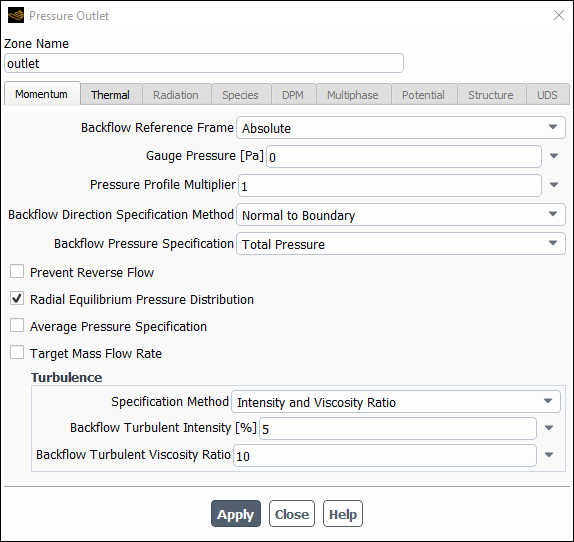
Controls
- Zone Name
sets the name of the zone.
- Momentum
contains the momentum parameters.
- Backflow Reference Frame
specify whether backflow temperature, pressure, and flow directions are in the Absolute or Relative to the Adjacent Cell Zone reference frame.
- Gauge Pressure
sets the gauge pressure at the outflow boundary.
- Pressure Profile Multiplier
sets a factor by which the Gauge Pressure is multiplied. This is provided mainly for cases where a non-uniform distribution of the static pressure at the pressure outlet boundary is specified by means of a profile file or a user-defined function.
- Backflow Direction Specification Method
sets the direction of the inflow stream should the flow reverse direction. If you choose Direction Vector, you will define the flow direction components, and if you choose Normal to Boundary or From Neighboring Cell, no inputs are required. You also have the option to enable Prevent Reverse Flow. See Inputs at Pressure Outlet Boundaries for information on specifying flow direction.
- Coordinate System
contains a drop-down list for selecting the coordinate system. You can choose Cartesian, Cylindrical, or Local Cylindrical. This option is available only when Direction Vector is selected from the Backflow Direction Specification Method drop-down list.
- X-, Y-, Z-Component of Flow Direction
allows you to specify the velocity components in x, y, and z directions respectively. This option is available when Cartesian is selected for the Coordinate System.
- Radial-, Tangential-, Axial-Component of Flow Direction
set the direction of the flow at the boundary. These items will appear for 2D axisymmetric cases, or for 3D cases for which the selected Coordinate System is Cylindrical or Local Cylindrical.
- Backflow Pressure Specification
specifies how the pressure is calculated under backflow conditions. When the NRBC option is not enabled, if you select Static Pressure, the Gauge Pressure is directly imposed as the boundary face pressure; if you select Total Pressure, the Gauge Pressure will be combined with a dynamic contribution that is based on the velocity in the adjacent cell zone. For NRBCs, if you select Static Pressure, the Gauge Pressure is directly imposed as the pressure at infinity; if you select Total Pressure, the pressure at infinity is a calculated value that is based on the Gauge Pressure.
- Radial Equilibrium Pressure Distribution
enables the radial equilibrium pressure distribution. See Defining Static Pressure for details.
This item appears only for 3D and axisymmetric swirl solvers.
- Average Pressure Specification
allows the pressure along the outlet boundary to vary, but maintain an average equivalent to the specified value in the Gauge Pressure input field. In this boundary implementation, the pressure variation provides a low level of non-reflectivity. For more details, see Calculation Procedure at Pressure Outlet Boundaries.
Note: The Average Pressure Specification option is not available if the Radial Equilibrium Pressure Distribution option is enabled.
- Target Mass Flow Rate
allows you to set mass flow rate as a boundary condition at the outlet.
- Target Mass Flow
allows you to specify the flow as either a constant value or a user-defined function.
- Upper Limit of Absolute Pressure, Lower Limit of Absolute Pressure
specifies the range of the pressure limits, which have different pressure variations on different boundaries. The upper and lower pressure limits can be specified as a constant or a profile.
- Turbulence
contains the turbulence parameters.
- Specification Method
specifies which method will be used to define the turbulence parameters. You can choose K and Epsilon (
 -
-  models and RSM only), K and Omega
(
models and RSM only), K and Omega
( -
-  models only), Intensity and Length Scale,
Intensity and Viscosity Ratio, Intensity and Hydraulic
Diameter, Modified Turbulent Viscosity (Spalart-Allmaras
model only), or Turbulent Viscosity Ratio (Spalart-Allmaras model
only). See Determining Turbulence Parameters for information about the inputs for each
of these methods. (This item will appear only for turbulent flow calculations.)
models only), Intensity and Length Scale,
Intensity and Viscosity Ratio, Intensity and Hydraulic
Diameter, Modified Turbulent Viscosity (Spalart-Allmaras
model only), or Turbulent Viscosity Ratio (Spalart-Allmaras model
only). See Determining Turbulence Parameters for information about the inputs for each
of these methods. (This item will appear only for turbulent flow calculations.)- Backflow Turbulent Kinetic Energy, Backflow Turbulent Dissipation Rate
set values for the turbulence kinetic energy
 and its dissipation rate
  . These items will appear if you choose K and
Epsilon as the Specification Method.
. These items will appear if you choose K and
Epsilon as the Specification Method.- Backflow Turbulent Kinetic Energy, Backflow Specific Dissipation Rate
set values for the turbulence kinetic energy
 and its specific dissipation rate
  . These items will appear if you choose K and
Omega as the Specification Method.
. These items will appear if you choose K and
Omega as the Specification Method.- Backflow Turbulent Intensity, Backflow Turbulent Length Scale
set values for turbulence intensity
 and turbulence length scale
  . These items will appear if you choose Intensity and Length
Scale as the Specification Method.
. These items will appear if you choose Intensity and Length
Scale as the Specification Method.- Backflow Turbulent Intensity, Backflow Turbulent Viscosity Ratio
set values for turbulence intensity
 and turbulent viscosity ratio
  . These items will appear if you choose Intensity and
Viscosity Ratio as the Specification Method.
. These items will appear if you choose Intensity and
Viscosity Ratio as the Specification Method.- Backflow Turbulent Intensity, Backflow Hydraulic Diameter
set values for turbulence intensity
 and hydraulic diameter
  . These items will appear if you choose Intensity and
Hydraulic Diameter as the Specification Method.
. These items will appear if you choose Intensity and
Hydraulic Diameter as the Specification Method.- Backflow Modified Turbulent Viscosity
sets the value of the backflow modified turbulent viscosity
 . This item will appear if you choose Modified Turbulent
Viscosity as the Specification Method.
. This item will appear if you choose Modified Turbulent
Viscosity as the Specification Method.- Backflow Turbulent Viscosity Ratio
sets the value of the backflow turbulent viscosity ratio
 . This item will appear if you choose Turbulent Viscosity
Ratio as the Specification Method.
. This item will appear if you choose Turbulent Viscosity
Ratio as the Specification Method.- Reynolds-Stress Specification Method
specifies which method will be used to determine the backflow Reynolds stress boundary conditions when the Reynolds stress turbulence model is used. You can choose either K or Turbulent Intensity or Reynolds-Stress Components. If you choose the former, Ansys Fluent will compute the Reynolds stresses for you. If you choose the latter, you will explicitly specify the Reynolds stresses yourself. See Reynolds Stress Model for details. (This item will appear only for RSM turbulent flow calculations.)
- Backflow UU, VV, WW, UV, VW, UW Reynolds Stresses
specify the backflow Reynolds stress components when Reynolds-Stress Components is chosen as the Reynolds-Stress Specification Method.
- Acoustic Wave Model
contains settings for treatment of acoustic pressure waves at the boundary.
- Off
disables special treatment of acoustic pressure waves at the boundary.
- Non Reflecting
enables the general non-reflecting boundary condition treatment described in General Non-Reflecting Boundary Conditions.
- Impedance
enables the impedance boundary condition treatment described in Impedance Boundary Conditions.
- Transparent Flow Forcing
enables the transparent flow forcing boundary condition described in Transparent Flow Forcing Boundary Conditions.
- Non Reflecting Parameters
contains settings for the non-reflecting boundary condition treatment.
- Exit Pressure Specification
defines how the pressure is calculated. For Pressure at Infinity, the pressure at the boundary relaxes toward the Gauge Pressure at infinity; for Average Boundary Pressure, an effort is made to force the average pressure on the boundary to approach the Gauge Pressure value.
- Impedance Parameters
contains the parameters for the impedance boundary condition treatment. For details refer to Using the Impedance Boundary Condition.
- Transparent Flow Forcing Parameters
contains the parameters for the transparent flow forcing boundary condition treatment. For details refer to Using the Transparent Flow Forcing Boundary Condition.
- Thermal
contains the thermal parameters.
- Backflow Total Temperature
sets the total temperature of the inflow stream should the flow reverse direction
- Radiation
contains the boundary conditions for the radiation model at the pressure outlet.
- External Black Body Temperature Method, Internal Emissivity
set the radiation boundary conditions when you are using the P-1, DTRM, DO, S2S, or MC models for radiation heat transfer. See Defining Boundary Conditions for Radiation for details.
- Participates in Solar Ray Tracing
specifies whether or not the pressure outlet participates in solar ray tracing.
- Solar Transmissivity Factor
specifies a multiplier (ranging from 0 to 1) that is applied to the solar irradiation entering the domain through the pressure outlet.
- Participates in View Factor Calculation
specifies whether or not the pressure outlet participates in the view factor calculation as part of the S2S radiation model. This parameter is available only if you select the Surface to Surface radiation model.
- Species
contains the species parameters.
- Specify Species in Mole Fractions
allows you to specify the species in mole fractions rather than mass fractions.
- Mean Mixture Fraction, Mixture Fraction Variance
set inlet values for the PDF mixture fraction and its variance. (These items will appear only if you are using the non-premixed or partially premixed combustion model.)
- Secondary Mean Mixture Fraction, Secondary Mixture Fraction Variance
set inlet values for the secondary mixture fraction and its variance. (These items will appear only if you are using the non-premixed or partially premixed combustion model with two mixture fractions.)
- Species Mass Fractions
contains inputs for the mass fractions of defined species. See Defining Cell Zone and Boundary Conditions for Species for details about these inputs. These items will appear only if you are modeling non-reacting multi-species flow or you are using the finite-rate reaction formulation.
- Backflow Progress Variable
sets the value of the progress variable for premixed turbulent combustion. See Setting Boundary Conditions for the Progress Variable for details.
This item will appear only if the premixed or partially premixed combustion model is used.
- Scalar Mass Fractions
(partially-premixed combustion FGM model only) allows you to specify the scalar species mass fractions for the transported scalars that you selected in the Select Transported Scalars dialog box.
- DPM
contains the discrete phase parameters.
- Discrete Phase BC Type
sets the way that the discrete phase behaves with respect to the boundary. This item appears when one or more injections have been defined.
- reflect
rebounds the particle off the boundary with a change in its momentum as defined by the coefficient of restitution. (See Particle Reflection at Wall in the Fluent Theory Guide.)
- trap
terminates the trajectory calculations and records the fate of the particle as "trapped". In the case of evaporating droplets, their entire mass instantaneously passes into the vapor phase and enters the cell adjacent to the boundary. See Figure 24.40: “Trap” Boundary Condition for the Discrete Phase.
- escape
reports the particle as having "escaped" when it encounters the boundary. Trajectory calculations are terminated. See Figure 24.41: “Escape” Boundary Condition for the Discrete Phase.
- reinject
reintroduces the particle into the domain when it reaches a certain domain boundary (for example, outlet). This item appears when one or more injections have been defined and Unsteady Particle Tracking is enabled in the Discrete Phase Model dialog box. See The reinject Boundary Condition for details.
- wall-jet
indicates that the direction and velocity of the droplet particles are given by the resulting momentum flux, which is a function of the impingement angle. See Figure 12.6: "Wall Jet" Boundary Condition for the Discrete Phase in the Theory Guide.
- user-defined
specifies a user-defined function to define the discrete phase boundary condition type.
- Discrete Phase BC Function
sets the user-defined function from the drop-down list.
- Multiphase
contains the multiphase parameters.
- Backflow Granular Temperature
specifies temperature for the solids phase and is proportional to the kinetic energy of the random motion of the particles. This option is available only for a granular phase with the Mixture and Eulerian multiphase models.
- Volume Fraction Specification Method
sets the method used to specify the volume fraction of the secondary phase selected in the Boundary Conditions Task Page. This section of the dialog box will appear when one of the multiphase models is being used. See Defining Multiphase Cell Zone and Boundary Conditions for details. This control is not available for the open channel VOF submodel.
- Backflow Volume Fraction
specifies the volume fraction of the secondary phase as a constant, profile, of UDF function.
- From Neighboring Cell
calculates the volume fraction from the neighboring cells.
- Open Channel
(VOF model only) enables the open-channel flow boundary condition. See Modeling Open Channel Flows for more information. This option is available only when the Open Channel VOF submodel is selected in the Multiphase Model dialog box. Once you select this option, you can specify the following conditions:
- Outlet Group ID
is used to identify the different outlets that are part of the same outlet group. See Setting the Outlet Group for details.
- Pressure Specification Method
specifies which method will be used to define the boundary conditions at the open-channel pressure outlet. You can choose from the following options:
Free Surface Level
From Neighboring Cell
Gauge Pressure
Refer to Pressure Outlet in the Fluent Theory Guide for more details.
- Secondary Phase for Level Specification
allows you to choose the desired secondary phase. This control is available only for flow applications with more than two phases.
- Free Surface Level
can be determined by using the absolute value of height from the free surface to the origin in the direction of gravity and applying the correct sign based on whether the free surface level is above (positive) or below (negative) the origin. See Determining the Free Surface Level for details.
- Bottom Level
is used for calculating the liquid height. It can be determined as described in Determining the Bottom Level.
- Density Interpolation Method
allows you to specify whether the mixture density used in the hydrostatic profile will be interpolated using the From Neighboring Cell, From Free Surface Level, or Hybrid method. See Choosing the Density Interpolation Method for more information. This drop-down list is available for sub-critical two-phase flow applications.
- Potential
displays the boundary conditions for the electric potential field. This tab is available only if you have enabled either the Electric Potential model or the Electrochemical reaction model in the Species Dialog Box.
- Potential Boundary Condition
is a drop-down list of available potential boundary condition types for the potential generated by electron current: Specified Flux and Specified Value. For the Specified Flux boundary condition, you will need to specify Current Density at the wall. For the Specified Value boundary condition, you will need to specify Potential at the wall.
- Electrolyte Potential Boundary Condition
is a drop-down list of available boundary condition types for the potential generated by ionic current. This item is similar to the Potential Boundary Condition drop-down list described above and is available only for the Electrolysis and H2 Pump model.
- UDS
contains the UDS parameters.
- User-Defined Scalar Boundary Condition
appears only if user-defined scalars are specified.
- User Scalar n
specifies whether the scalar is a specified flux or a specified value.
- User-Defined Scalar Boundary Value
appears only if user-defined scalars are specified.
- User Scalar n
specifies the value of the scalar.
The Radiator dialog box sets the boundary conditions for a radiator model zone. It is opened from the Boundary Conditions Task Page. See User Inputs for Radiators for details about the items below.
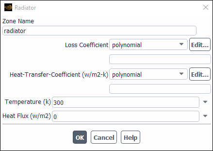
Controls
- Zone Name
sets the name of the zone.
- Loss Coefficient
specifies the loss coefficient as a constant value or as a polynomial, piecewise-linear, or piecewise-polynomial function of velocity. See Defining the Pressure Loss Coefficient Function for details.
- Heat-Transfer-Coefficient
specifies the heat-transfer coefficient as a constant value or as a polynomial, piecewise-linear, or piecewise-polynomial function of velocity. See Defining the Heat Flux Parameters for details.
- Temperature
sets the temperature used to compute heat flux from the radiator using the Heat-Transfer-Coefficient. If Temperature is absolute zero, the Heat Flux condition is used instead.
- Heat Flux
sets the heat flux at the radiator surface (used only when Temperature is absolute zero).
- Discrete Phase BC Type
sets the way that the discrete phase behaves with respect to the boundary. This item appears when one or more injections have been defined.
- interior
allows the particles to pass through the boundary.
- reflect
rebounds the particle off the boundary with a change in its momentum as defined by the coefficient of restitution. (See Particle Reflection at Wall in the Fluent Theory Guide.)
- trap
terminates the trajectory calculations and records the fate of the particle as "trapped". In the case of evaporating droplets, their entire mass instantaneously passes into the vapor phase and enters the cell adjacent to the boundary. See Figure 24.40: “Trap” Boundary Condition for the Discrete Phase.
- escape
reports the particle as having "escaped" when it encounters the boundary. Trajectory calculations are terminated. See Figure 24.41: “Escape” Boundary Condition for the Discrete Phase.
- reinject
reintroduces the particle into the domain when it reaches a certain domain boundary (for example, outlet). This item appears when one or more injections have been defined and Unsteady Particle Tracking is enabled in the Discrete Phase Model dialog box. See The reinject Boundary Condition for details.
- wall-jet
indicates that the direction and velocity of the droplet particles are given by the resulting momentum flux, which is a function of the impingement angle. See Figure 12.6: "Wall Jet" Boundary Condition for the Discrete Phase in the Theory Guide.
- user-defined
specifies a user-defined function to define the discrete phase boundary condition type.
- Discrete Phase BC Function
sets the user-defined function from the drop-down list.
The RANS/LES Interface dialog box can be used to create artificial resolved turbulence (fluctuation/perturbations) at the interface where the flow proceeds from the RANS zone into the LES zone of the computational domain for Embedded LES turbulent flows. It is opened from the Boundary Conditions Task Page. See Setting Up the Embedded Large Eddy Simulation (ELES) Model for more information about RANS/LES interfaces.
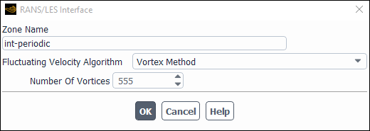
Controls
- Zone Name
sets the name of the RANS/LES interface.
- Fluctuating Velocity Algorithm
displays the methods for generating fluctuating velocity components at the RANS/LES interface. Available options include:
No Perturbations
Spectral Synthesizer
Vortex Method
- Number of Vortices
displays the amount of vortices that the selected fluctuating velocity method distributes randomly over the face zone and uses to generate turbulent fluctuations (available for the Vortex Method only).
Important: The RANS/LES 'interface' can either be an interior zone (that has been assigned to be a rans-les-interface zone), or it can be a non-conformal interface. If it is a non-conformal interface, then you need to identify the name of the non-conformal interface's "interior" zone (for example, using the button in the Mesh Interfaces Dialog Box), and then go to that zone in the Boundary Conditions task page.
The Symmetry dialog box can be used to modify the name of a symmetry zone; there are no conditions to be set. It is opened from the Boundary Conditions Task Page. See Symmetry Boundary Conditions for information about symmetry boundaries.
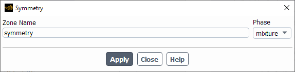
Controls
- Zone Name
sets the name of the zone.
- Phase
displays the name of the phase. This item is available only for multiphase flows.
The Velocity Inlet dialog box sets the boundary conditions for a velocity inlet zone. It is opened from the Boundary Conditions Task Page. See Inputs at Velocity Inlet Boundaries for details about defining the items below.
Important: This feature offers reduced functionality when running Fluent under the Pro capability level.
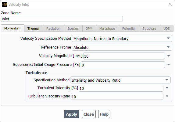
Controls
- Zone Name
sets the name of the zone.
- Phase
displays the name of the phase. This item appears if the VOF, mixture, or Eulerian multiphase model is being used.
- Open Channel Wave BC
allows you to set specific parameters for a particular boundary for open channel wave boundaries. This is available when the volume of fluid multiphase model is selected.
- Momentum
contains the momentum parameters.
- Velocity Specification Method
sets the method used to define the inflow velocity.
- Flow Direction Specification Method
sets the method used to define the direction of flow of the wave. This is available when you enable the Open Channel Wave BC option.
- Magnitude and Direction
allows specification in terms of a Velocity Magnitude and Flow-Direction.
- Components
allows specification in terms of the Cartesian, cylindrical, or local cylindrical velocity components.
- Magnitude, Normal to Boundary
allows specification of a Velocity Magnitude normal to the boundary.
- Reference Frame
specifies relative or absolute velocity inputs. You can choose to enter Absolute velocities or velocities Relative to Adjacent Cell Zone. If you are not using moving reference frames, both options are equivalent, so you need not choose.
- Uniform Flow Velocity Magnitude
is the flow velocity, specified as a constant or a parameter.
- Coordinate System
specifies whether Cartesian, Cylindrical, or Local Cylindrical velocities will be defined. This item will appear only for 3D cases in which you have selected Magnitude and Direction or Components as the Velocity Specification Method.
- X-, Y-, Z-Velocity
set the components of the velocity vector at the inflow boundary. These items will appear for 2D non-axisymmetric models, or for 3D models if you select the Components option as the Velocity Specification Method and Cartesian as the Coordinate System.
- Radial-, Tangential-, Axial-Velocity
set the components of the velocity vector at the inflow boundary. These items will appear for 3D models if you select the Components option as the Velocity Specification Method and Cylindrical or Local Cylindrical as the Coordinate System.
- Axial-, Radial-, Swirl-Velocity
set the components of the velocity vector at the inflow boundary. These items will appear for 2D axisymmetric models.
Important: Swirl-Velocity will appear only for 2D axisymmetric swirl models.
- Angular Velocity
specifies the angular velocity
 for a 3D flow. This item will appear for a 3D model if you select the
Components option as the Velocity Specification
Method and Cylindrical or Local
Cylindrical as the Coordinate System.
for a 3D flow. This item will appear for a 3D model if you select the
Components option as the Velocity Specification
Method and Cylindrical or Local
Cylindrical as the Coordinate System.- Swirl Angular Velocity
specifies the swirl angular velocity
 for an axisymmetric swirling flow. This item will appear for an
axisymmetric swirl model if you choose Components as the
Velocity Specification Method.
for an axisymmetric swirling flow. This item will appear for an
axisymmetric swirl model if you choose Components as the
Velocity Specification Method.- Velocity Magnitude
sets the magnitude of the velocity vector at the inflow boundary. This item will appear if you select the Magnitude and Direction or Magnitude, Normal to Boundary option as the Velocity Specification Method.
- X-, Y-, Z-Component of Flow Direction
set the direction of the velocity vector at the inflow boundary. These items will appear for 2D non-axisymmetric models if you select the Magnitude and Direction option as the Velocity Specification Method, or for 3D models if you select the Magnitude and Direction option as the Velocity Specification Method and Cartesian as the Coordinate System.
- Radial-, Tangential-, Axial-Component of Flow Direction
set the direction of the velocity vector at the inlet boundary. These items will appear for 3D models if you select the Magnitude and Direction option as the Velocity Specification Method and Cylindrical or Local Cylindrical as the Coordinate System, or for 2D axisymmetric models.
Important: Tangential-Velocity will appear only for 2D axisymmetric swirl models.
- Axis Origin
sets the X, Y, and Z coordinates of the origin of the local cylindrical coordinate system.
- Axis Direction
sets the X, Y, and Z components of the direction of the local cylindrical coordinate system.
- Outflow Gauge Pressure
specifies the pressure to be used as the pressure outlet condition if flow exits the domain at any face on the velocity inlet boundary. (Note that this effect is similar to that of the "velocity far-field" boundary that was available in RAMPANT 3.)
This item appears only for the density-based solvers.
- Fluctuating Velocity
contains parameters for Inlet Boundary Conditions for Scale Resolving Simulations (only available for transient cases where scale-resolving turbulence models such as SAS, DES, and LES are enabled).
- Fluctuating Velocity Algorithm
Specifies which method will be used for generating fluctuations at the boundary for Scale Resolving Simulations. The following methods are available:
- No Perturbations
No fluctuations added.
- Vortex Method
For details, see Vortex Method in the Fluent Theory Guide.
- Spectral Synthesizer
For details, see Spectral Synthesizer in the Fluent Theory Guide.
- Synthetic Turbulence Generator
For details, see Synthetic Turbulence Generator in the Fluent Theory Guide.
- Number of Vortices
Specifies number of vortices to be generated with the Vortex Method.
- Satisfy Mass Conservation?
Enables mass conservation for the Vortex Method at the boundary.
- Scale Search Limiter
Specifies which method will be used to limit the area from where global scales for the Synthetic Turbulence Generator are computed. The following methods are available:
- None
Scales are computed using the entire inlet zone.
- Turbulent Intensity Threshold
Scales are computed using only part of the inlet zone where Turbulent Intensity is higher than specified threshold value.
- Turbulent Viscosity Ratio Threshold
Scales are computed using only part of the inlet zone where Turbulent Viscosity Ratio is higher than specified threshold value.
- Wall Distance Threshold
Scales are computed using only part of the inlet zone where Wall Distance is smaller than specified threshold value.
- Turbulent Intensity, Turbulent Viscosity Ratio, or Wall Distance
Specifies threshold value for the corresponding Scale Search Limiter (only available for the Synthetic Turbulence Generator with corresponding Scale Search Limiter chosen).
- Volumetric Forcing?
Enables generation of fluctuations in the volume adjacent to the inlet boundary instead of introduction of fluctuations directly at the boundary (only available for the Synthetic Turbulence Generator).
- Forcing Zone Thickness
Specifies which method will be used to set up the streamwise size of the volume where fluctuations are to be generated (only available for the Synthetic Turbulence Generator with Volumetric Forcing? enabled). The following methods are available:
- Automatic
Length is computed based on the turbulent length scale computed from the boundary.
- Specified Value
Length is specified by the user.
- Thickness
Specifies the streamwise size of the volume where fluctuations are to be generated (only available for the Synthetic Turbulence Generator with Volumetric Forcing? enabled if Specified Value option is chosen for Forcing Zone Thickness).
- Turbulence
contains the turbulence parameters.
- Specification Method
specifies which method will be used to define the turbulence parameters. You can choose K and Epsilon (
 -
-  models and RSM only), K and Omega
(
models and RSM only), K and Omega
( -
-  models only), Intensity and Length Scale,
Intensity and Viscosity Ratio, Intensity and Hydraulic
Diameter, Modified Turbulent Viscosity (Spalart-Allmaras
model only), or Turbulent Viscosity Ratio (Spalart-Allmaras model
only). See Determining Turbulence Parameters for information about the inputs for each
of these methods. (This item will appear only for turbulent flow calculations.)
models only), Intensity and Length Scale,
Intensity and Viscosity Ratio, Intensity and Hydraulic
Diameter, Modified Turbulent Viscosity (Spalart-Allmaras
model only), or Turbulent Viscosity Ratio (Spalart-Allmaras model
only). See Determining Turbulence Parameters for information about the inputs for each
of these methods. (This item will appear only for turbulent flow calculations.)- Turbulent Kinetic Energy, Turbulent Dissipation Rate
set values for the turbulence kinetic energy
 and its dissipation rate
  . These items will appear if you choose K and
Epsilon as the Specification Method.
. These items will appear if you choose K and
Epsilon as the Specification Method.- Turbulent Kinetic Energy, Specific Dissipation Rate
set values for the turbulence kinetic energy
 and its specific dissipation rate
  . These items will appear if you choose K and
Omega as the Specification Method.
. These items will appear if you choose K and
Omega as the Specification Method.- Turbulent Intensity, Turbulent Length Scale
set values for turbulence intensity
 and turbulence length scale
  . These items will appear if you choose Intensity and Length
Scale as the Specification Method.
. These items will appear if you choose Intensity and Length
Scale as the Specification Method.- Turbulent Intensity, Turbulent Viscosity Ratio
set values for turbulence intensity
 and turbulent viscosity ratio
  . These items will appear if you choose Intensity and
Viscosity Ratio as the Specification Method.
. These items will appear if you choose Intensity and
Viscosity Ratio as the Specification Method.- Turbulent Intensity, Hydraulic Diameter
set values for turbulence intensity
 and hydraulic diameter
  . These items will appear if you choose Intensity and
Hydraulic Diameter as the Specification Method.
. These items will appear if you choose Intensity and
Hydraulic Diameter as the Specification Method.- Modified Turbulent Viscosity
sets the value of the modified turbulent viscosity
 . This item will appear if you choose Modified Turbulent
Viscosity as the Specification Method.
. This item will appear if you choose Modified Turbulent
Viscosity as the Specification Method.- Turbulent Viscosity Ratio
sets the value of the turbulent viscosity ratio
 . This item will appear if you choose Turbulent Viscosity
Ratio as the Specification Method.
. This item will appear if you choose Turbulent Viscosity
Ratio as the Specification Method.- Turbulent Intensity
sets the value of the turbulence intensity
 for the LES model.
- Reynolds-Stress Specification Method
specifies which method will be used to determine the Reynolds stress boundary conditions when the Reynolds stress turbulence model is used. You can choose either K or Turbulent Intensity or Reynolds-Stress Components. If you choose the former, Ansys Fluent will compute the Reynolds stresses for you. If you choose the latter, you will explicitly specify the Reynolds stresses yourself. See Reynolds Stress Model for details. (This item will appear only for RSM turbulent flow calculations.)
- UU, VV, WW, UV, VW, UW Reynolds Stresses
specify the Reynolds stress components when Reynolds-Stress Components is chosen as the Reynolds-Stress Specification Method.
- Acoustic Wave Model
contains settings for treatment of acoustic pressure waves at the boundary.
- Off
disables special treatment of acoustic pressure waves at the boundary.
- Non Reflecting
enables the general non-reflecting boundary condition treatment described in General Non-Reflecting Boundary Conditions.
- Impedance
enables the impedance boundary condition treatment described in Impedance Boundary Conditions.
- Transparent Flow Forcing
enables the transparent flow forcing boundary condition described in Transparent Flow Forcing Boundary Conditions.
- Impedance Parameters
contains the parameters for the impedance boundary condition treatment. For details refer to Using the Impedance Boundary Condition.
- Transparent Flow Forcing Parameters
contains the parameters for the transparent flow forcing boundary condition treatment. For details refer to Using the Transparent Flow Forcing Boundary Condition.
- Thermal
contains the thermal parameters.
- Temperature
specifies the static temperature of the flow.
- Radiation
contains the boundary conditions for the radiation model at the velocity inlet.
- External Black Body Temperature Method, Internal Emissivity
set the radiation boundary conditions when you are using the P-1, DTRM, DO, S2S, or MC models for radiation heat transfer. See Defining Boundary Conditions for Radiation for details.
- Participates in Solar Ray Tracing
specifies whether or not the velocity inlet participates in solar ray tracing.
- Solar Transmissivity Factor
specifies a multiplier (ranging from 0 to 1) that is applied to the solar irradiation entering the domain through the velocity inlet.
- Participates in View Factor Calculation
specifies whether or not the velocity inlet participates in the view factor calculation as part of the S2S radiation model. This parameter is available only if you select the Surface to Surface radiation model.
- Species
contains the species parameters.
- Specify Species in Mole Fractions
allows you to specify the species in mole fractions rather than mass fractions.
- Species Mass Fractions
contains inputs for the mass fractions of defined species. See Defining Cell Zone and Boundary Conditions for Species for details about these inputs. These items will appear only if you are modeling non-reacting multi-species flow or you are using the finite-rate reaction formulation.
- Mean Mixture Fraction, Mixture Fraction Variance
set inlet values for the PDF mixture fraction and its variance. These items will appear only if you are using the non-premixed or partially premixed combustion model.
- Secondary Mean Mixture Fraction, Secondary Mixture Fraction Variance
set inlet values for the secondary mixture fraction and its variance. (These items will appear only if you are using the non-premixed or partially premixed combustion model with two mixture fractions.)
- Progress Variable
sets the value of the progress variable for premixed turbulent combustion. See Setting Boundary Conditions for the Progress Variable for details.
This item will appear only if the premixed or partially premixed combustion model is used.
- Scalar Mass Fractions
(partially-premixed combustion FGM model only) allows you to specify the scalar species mass fractions for the transported scalars that you selected in the Select Transported Scalars dialog box.
- DPM
contains the discrete phase parameters.
- Discrete Phase BC Type
sets the way that the discrete phase behaves with respect to the boundary. This item appears when one or more injections have been defined.
- reflect
rebounds the particle off the boundary with a change in its momentum as defined by the coefficient of restitution. (See Particle Reflection at Wall in the Fluent Theory Guide.)
- trap
terminates the trajectory calculations and records the fate of the particle as "trapped". In the case of evaporating droplets, their entire mass instantaneously passes into the vapor phase and enters the cell adjacent to the boundary. See Figure 24.40: “Trap” Boundary Condition for the Discrete Phase.
- escape
reports the particle as having "escaped" when it encounters the boundary. Trajectory calculations are terminated. See Figure 24.41: “Escape” Boundary Condition for the Discrete Phase.
- reinject
reintroduces the particle into the domain when it reaches a certain domain boundary (for example, outlet). This item appears when one or more injections have been defined and Unsteady Particle Tracking is enabled in the Discrete Phase Model dialog box. See The reinject Boundary Condition for details.
- wall-jet
indicates that the direction and velocity of the droplet particles are given by the resulting momentum flux, which is a function of the impingement angle. See Figure 12.6: "Wall Jet" Boundary Condition for the Discrete Phase in the Theory Guide.
- user-defined
specifies a user-defined function to define the discrete phase boundary condition type.
- Discrete Phase BC Function
sets the user-defined function from the drop-down list.
- Multiphase
contains the multiphase parameters.
- Volume Fraction
specifies the volume fraction of the secondary phase selected in the Boundary Conditions Task Page. This section of the dialog box will appear when one of the multiphase models is being used. See Defining Multiphase Cell Zone and Boundary Conditions for details.
- Secondary Phase for Inlet
specifies the secondary phase to which the parameters are applied. In case of a three-phase flow, select the corresponding secondary phase from this list.
- Wave BC Options
allows you to choose between Shallow Waves, Shallow/Intermediate Waves or Short Gravity Waves. Information about the two types of waves is available in Open Channel Wave Boundary Conditions in the Theory Guide.
- Free Surface Level
is determined by using the absolute value of height from the free surface to the origin in the direction of gravity and applying the correct sign based on whether the free surface level is above (positive) or below (negative) the origin.
- Bottom Level
is valid for shallow and intermediate waves. The bottom level is used for calculating the liquid height.
- Reference Wave Direction
is the direction of wave propagation for a zero wave heading angle.
- Wave Modeling Options
determines whether to use wave theory or a wave spectrum to model waves in the shallow/intermediate and short gravity wave regimes.
- Number of Waves
specifies the number of waves you are defining when modeling waves using wave theory.
- Wave Theory
allows you to choose from First Order Airy (the default), Second Order Stokes, Third Order Stokes, Fourth Order Stokes, and Fifth Order Stokes for shallow/intermediate waves and short gravity waves. For shallow waves, you can choose between Fifth Order Solitary and Fifth Order Cnoidal. Information about the types of wave theory is available in Open Channel Wave Boundary Conditions in the Theory Guide.
- Wave Height
is the height difference between a wave crest to the neighboring trough.
Since a solitary wave does not have troughs, the wave height is the distance between a wave crest to mean free surface level.
- Wave Length
is the wave length of the shallow wave or short gravity wave.
- Inlet Offset Distance
is the translational distance from the reference point origin in the reference wave propagation direction. This option is used to generate a wave from a location other than the reference frame origin.
- Phase Difference
is the phase difference between one wave and another.
- Wave Heading Angle
is the angle between the direction of the wavefront and the reference wave direction, in the plane of the flow surface. In 2D, there are only two possibilities, zero degrees when the wave is in the reference wave direction, and 180 degrees when the wave is in the opposite direction.
- Frequency Spectrum Method
specifies the spectrum to use. You can select Pierson-Moskowitz (appropriate for fully-developed seas), Jonswap (appropriate for fetch-limited seas), or TMA (appropriate for fetch-limited, finite-depth seas).
- Peak Shape Parameter
controls the shape and amplitude of the frequency peak in the Jonswap and TMA formulations. This corresponds to
 in Equation 14–101 in the Fluent Theory Guide.
- Significant Wave Height
is the mean wave height of the largest 1/3 of waves. This corresponds to
 in Equation 14–100 in the Fluent Theory Guide.
- Peak Wave Frequency
is the wave frequency corresponding to the highest wave energy. This corresponds to
 in Equation 14–100 and Equation 14–101 in the Fluent Theory Guide.
  can be expressed in terms of the peak wave period,
  , as
, as  .
.- Minimum/Maximum Wave Frequency
specify the frequency range for the spectrum. Note that the Peak Wave Frequency must fall in between Minimum Wave Frequency and .
- Number of Frequency Components
specifies the number of components into which the frequency spectrum is divided.
specifies the method to use for specifying the directional spreading characteristics. You can choose Unidirectional (for long-crested waves), Frequency Independent Cosine Function (for short-crested waves where the directional component does not depend on frequency), and Frequency Dependant Hyperbolic Function (for short-crested waves where the directional component depends on frequency).
- Frequency Independent Cosine Exponent
specifies the exponent in the Frequency Independent Cosine Function formulation. This corresponds to
 in Equation 14–105 in the Fluent Theory Guide.
- Mean Wave Heading Angle
specifies the principal wave heading direction.
- Angular Spread
specifies the deviation from the mean wave direction for calculating the angular range.
- Number of Angular Components
specifies the number of components into which the angular range is divided.
- Potential
displays the boundary conditions for the electric potential field. This tab is available only if you have enabled either the Electric Potential model or the Electrochemical reaction model in the Species Dialog Box.
- Potential Boundary Condition
is a drop-down list of available potential boundary condition types for the potential generated by electron current: Specified Flux and Specified Value. For the Specified Flux boundary condition, you will need to specify Current Density at the wall. For the Specified Value boundary condition, you will need to specify Potential at the wall.
- Electrolyte Potential Boundary Condition
is a drop-down list of available boundary condition types for the potential generated by ionic current. This item is similar to the Potential Boundary Condition drop-down list described above and is available only for the Electrolysis and H2 Pump model.
- UDS
contains the UDS parameters.
- User-Defined Scalar Boundary Condition
appears only if user-defined scalars are specified.
- User Scalar n
specifies whether the scalar is a specified flux or a specified value.
- User-Defined Scalar Boundary Value
appears only if user-defined scalars are specified.
- User Scalar n
specifies the value of the scalar.
The Wall dialog box sets the boundary conditions for a wall zone. It is opened from the Boundary Conditions Task Page. See Inputs at Wall Boundaries for details about defining the items below.
Important: This feature offers reduced functionality when running Fluent under the Pro capability level.
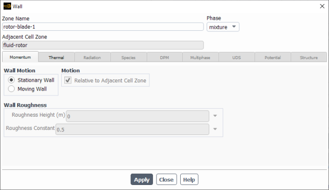
Controls
- Zone Name
sets the name of the zone.
- Phase
displays the name of the phase. This item appears if the VOF, mixture, or Eulerian multiphase model is being used.
- Adjacent Cell Zone
shows the name of the cell zone adjacent to the wall. (This is for informational use only; you cannot edit this field.)
- Momentum
displays the momentum boundary conditions.
- Wall Motion
contains options for specifying whether or not the wall is moving.
- Stationary Wall
specifies that the wall is not moving relative to the adjacent cell zone.
- Moving Wall
enables specification of the tangential wall motion. Tangential wall motion is applicable only to viscous flows. Since the inviscid slip condition decouples the tangential wall velocity from the governing equations, tangential wall motion has no effect on inviscid flow.
- Motion
contains inputs related to wall motion. See Velocity Conditions for Moving Walls for details.
- Relative to Adjacent Cell Zone
enables the specification of a wall velocity relative to the velocity of the adjacent cell zone.(If the adjacent cell zone is not moving, this is equivalent to Absolute.)
- Absolute
enables the specification of an absolute wall velocity,
- Translational
enables the specification of a translational wall velocity.
- Rotational
enables the specification of a rotational wall velocity.
- Components
enables the specification of wall velocity components.
- Speed
sets the translational or rotational speed of the wall (depending on whether you selected Translational or Rotational).
- Direction
sets the direction vector of the translational velocity. (This item will appear if you have chosen the Translational option.)
- Rotation-Axis Origin
sets the coordinates of the origin of the axis of rotation, thereby determining the location of the axis. (This item will appear if you have chosen the Rotational option for a non-axisymmetric case.)
- Rotation-Axis Direction
sets the direction vector for the axis of rotation. (This item will appear if you have chosen the Rotational option for a non-axisymmetric case.)
- Velocity Components
sets the X, Y, and Z-Velocity components of the wall motion. (This item will appear if you have chosen the Components option.)
- Shear Condition
contains options for specifying the shear conditions at the wall.
- No Slip
specifies a no-slip condition at the wall. No further inputs are required.
- Specified Shear
enables specification of zero or nonzero shear. See Specified Shear for details. This option is not available for moving walls.
- Marangoni Stress
enables the specification of shear stress caused by the variation of surface tension due to temperature. This option is not available for moving walls.
- Shear Stress
contains inputs related to wall shear. These items will appear when Specified Shear is selected as the Shear Condition. See Specified Shear for details.
- X-Component, Y-Component, Z-Component, Swirl Component
specify the
 ,
,  , and
, and  or swirl components of shear for a slip wall. Swirl
Component is available only for axisymmetric swirl cases.
or swirl components of shear for a slip wall. Swirl
Component is available only for axisymmetric swirl cases.
- Specularity Coefficient
is used in multiphase granular flow. You can specify the specularity coefficient such that when the value is zero, this condition is equivalent to zero shear at the wall, but when the value is near unity, there is a significant amount of lateral momentum transfer.
- Specularity Coefficient
allows you to enter a value between zero and one, which controls the amount of lateral momentum transfer.
- Marangoni Stress
contains inputs related to Marangoni stress. This item will appear when Marangoni Stress is selected as the Shear Condition. See Marangoni Stress for details.
- Surface Tension Gradient
specifies the surface tension gradient with respect to temperature (
 in Equation 7–120).
- Wall Roughness
contains various models for defining wall roughness size/height in turbulent calculations.
- Standard
uses the standard wall roughness methods for most turbulence models. See Wall Roughness Effects in Turbulent Wall-Bounded Flows for details.
- High Roughness (Icing)
contains various models for use only with the Spalart-Allmaras and SST k-ω turbulence models. Specifically applicable to icing simulations, choose from Specified Roughness, NASA Correlation, Shin-et-al, or ICE3D Roughness File methods to specify the Sand-Grain Roughness. See Wall Roughness Effects in Turbulent Wall-Bounded Flows for details.
- Wall Adhesion
contains inputs related to wall adhesion. This section of the dialog box will appear if you are using the VOF model and have enabled Wall Adhesion in the e Multiphase Model Dialog Box (Forces tab).
- Contact Angles
specifies the contact angle at the wall for each pair of phases (
 in Figure 26.21: Measuring the Contact Angle in the Theory Guide). See Steps for Setting Boundary Conditions for details.
- Thermal
contains the thermal parameters. This tab is available only when the energy equation is turned on.
- Thermal Conditions
contains radio buttons for selecting the thermal boundary condition type. See Thermal Boundary Conditions at Walls for details about these inputs:
- Heat Flux
selects a specified heat flux condition.
- Temperature
selects a specified wall temperature condition.
- Convection
selects a convective heat transfer boundary condition model.
- Radiation
selects an external radiation boundary condition.
- Mixed
selects a combined convection/external radiation boundary condition.
- Coupled
selects a coupled heat transfer condition. It is applicable only to walls that form the interface between two regions (such as the fluid/solid interface for a conjugate heat transfer problem).
- via System Coupling
selects a heat transfer condition where a boundary can receive thermal data (either wall temperature, heat flow, or heat transfer coefficient) from the System Coupling service. It is applicable when Ansys Fluent is coupled with another system in Workbench using System Coupling (see Heat Transfer Boundary Conditions Through System Coupling for details).
- via Mapped Interface
specifies that the thermal data is interpolated across a mapped interface. It is available only for the interface wall boundary zones created as part of a mapped interface (see Heat Transfer Boundary Conditions Across a Mapped Interface for details).
Once a condition type has been selected, the appropriate conditions can be specified.
- Heat Flux
sets the wall heat flux to be used for the Heat Flux condition. A specification of zero Heat Flux is simply the adiabatic condition (no heat transfer). A positive value of heat flux implies that heat enters into the domain.
- Temperature
sets the wall temperature to be used for the Temperature condition.
- Heat Transfer Coefficient
sets the convective heat transfer coefficient to be used for the Convection condition (
 in Equation 7–127).
- Free Stream Temperature
sets the reference or free stream temperature to be used for the Convection condition (
 in Equation 7–127).
- External Emissivity
sets the emissivity of the external wall to be used for the Radiation condition (
 in Equation 7–128).
- External Radiation Temperature
sets the temperature of the external radiation source/sink to be used for the Radiation condition (
 in Equation 7–128).
- Wall Thickness
sets the thickness of a thin wall for the calculation of thermal resistance. (See Thin-Wall Thermal Resistance Parameters for details.)
- Heat Generation Rate
sets the rate of heat generation in a wall without shell conduction.
- Contact Resistance
sets the contact resistance (
 in Equation 15–23 in the Theory Guide) at the wall. See Modeling Solidification and Melting for details. This item appears only when the
solidification/melting model is used.
in Equation 15–23 in the Theory Guide) at the wall. See Modeling Solidification and Melting for details. This item appears only when the
solidification/melting model is used.- Material Name
sets the material type for a thin wall. The conductivity of the material is used for the calculation of thin-wall thermal resistance. (See Thin-Wall Thermal Resistance Parameters for details.) Material is used only when Wall Thickness is nonzero. Materials are defined with the Materials Task Page.
- Boundary Advection
enables the advection of heat into or out of the domain as a result of motion that is normal to the boundary. This option is only available for a boundary wall that is adjacent to a solid cell zone that undergoes solid motion. For details, see Boundary Advection for Solid Motion.
- Shell Conduction
enables shell conduction for the wall. See Shell Conduction for details.
- Edit...
is only available when Shell Conduction is enabled, and opens the Conduction Layers Dialog Box in order to allow you to define the shell conduction settings for the wall.
- Radiation
displays the boundary conditions for the S2S model, the DO model, the MC model, and the non-gray P-1 model at the wall. This tab is only available if you are using the surface to surface model, the discrete ordinates model, the Monte Carlo model, or the non-gray P-1 model. See Forming Surface Clusters, Wall Boundary Conditions for the DO Model, and Wall Boundary Conditions for the DTRM, P-1, S2S, and Rosseland Models for details.
- BC Type
contains a drop-down list of available radiation boundary condition types. The available options are opaque and semi-transparent. This item will appear only if you are using the discrete ordinates or Monte Carlo model.
- Boundary Source
enables the wall to be a radiation source. This is only available for external semi-transparent walls with the MC or DO models and for internal or external opaque walls with the MC model.
- Polar Distribution Function
enables a polar (rotationally symmetric about a given direction) boundary source which can be used if the irradiation intensity varies with direction such as in the case of LED light sources. The polar distribution function is defined by an Expression or by a table of data pairs consisting of an Angle and it's corresponding Relative Intensity. You have the option to read and write the polar data in the form of
.csvfiles or plotting the data in the graphics window. Only available with the MC model.- Reference Direction
Specify the (X,Y,Z) vector that defines the center of the polar distribution function. Only available with the MC model.
- Internal Emissivity
sets the internal emissivity of the wall. This item will appear only if you are using the P-1, DO, MC, DTRM, or S2S models for radiation heat transfer.
- Diffuse Fraction
specifies the fraction of the irradiation that is to be treated as diffuse. By default, the Diffuse Fraction is set to 1, indicating that all of the irradiation is diffuse. If the non-gray DO or MC model is being used, the Diffuse Fraction can be specified for each band. This item will appear only if you are using the Monte Carlo or discrete ordinates model.
- Beam Width
specifies the beam width for an external semi-transparent wall in terms of the Theta and Phi extents. This item will appear only if you are using the discrete ordinates radiation model and you have selected semi-transparent as the BC Type.
- Beam Direction
specifies the beam direction as an X,Y,Z vector. You can specify the Beam Direction as a constant, a profile, or a user-defined function. This item will appear only if you are using the Monte Carlo model or the discrete ordinates radiation model and you have selected semi-transparent as the BC Type.
- Direct Irradiation
specifies the value of the irradiation flux. If the non-gray DO or MC models are being used, a constant Direct Irradiation can be specified for each band.
This item will appear only if you are using the MC model or the semi-transparent BC Type with the DO model.
- Apply Direct Irradiation Parallel to the Beam
By default, Apply Direct Irradiation Parallel to the Beam is selected, which means Fluent assumes that the value you specify for Direct Irradiation is the irradiation flux parallel to the Beam Direction. When deselected, Ansys Fluent assumes that the value you specify for Direct Irradiation is the irradiation flux normal to the boundary.
- Apply Irradiation About the Reference Direction
By default, Apply Irradiation About the Reference Direction is selected, which means Fluent assumes that the value you specify for Direct Irradiation is the irradiation flux parallel to the Reference Direction. When deselected, Ansys Fluent assumes that the value you specify for Direct Irradiation is the irradiation flux normal to the boundary. See Figure 5.12: DO Irradiation on External Semi-Transparent Wall in Semi-Transparent Exterior Walls in the Theory Guide for details.
- Diffuse Irradiation
specifies the value of the irradiation flux. If the non-gray DO or MC model is being used, a constant Diffuse Irradiation can be specified for each band.
This item will appear only if you are using the DO or MC radiation model and you have selected semi-transparent as the BC Type.
- Solar Boundary Conditions
contains the settings for solar ray tracing. This group box is available only if you select Solar Ray Tracing from the Model list in the Solar Load group box of the Radiation Model dialog box. For semitransparent coupled walls, the solar ray tracing settings are defined on the original wall and not on the shadow wall. See Solar Ray Tracing for details.
- Participates in Solar Ray Tracing
specifies whether or not the wall participates in solar ray tracing.
- Absorptivity
contains the settings that define the absorptivity of wall.
- Direct Visible
specifies a multiplier (ranging from 0 to 1) that is applied to the visible portion of the direct solar radiation spectrum to account for the absorption of the wall. The value should be defined for normal incident rays.
- Direct IR
specifies a multiplier (ranging from 0 to 1) that is applied to the infrared portion of the direct solar radiation spectrum to account for the absorption of the wall. The value should be defined for normal incident rays.
- Diffuse Hemispherical
specifies a multiplier (ranging from 0 to 1) that is applied to the diffuse solar radiation to account for the absorption of the wall. This setting is only available for semi-transparent walls.
- Transmissivity
contains the settings that define the transmissivity of wall. This group box is only available when semi-transparent is selected for BC Type.
- Direct Visible
specifies a multiplier (ranging from 0 to 1) that is applied to the visible portion of the direct solar radiation spectrum to account for the transmissivity of the wall. The value should be defined for normal incident rays. This setting is only available for semi-transparent walls.
- Direct IR
specifies a multiplier (ranging from 0 to 1) that is applied to the infrared portion of the direct solar radiation spectrum to account for the transmissivity of the wall. The value should be defined for normal incident rays. This setting is only available for semi-transparent walls.
- Diffuse Hemispherical
specifies a multiplier (ranging from 0 to 1) that is applied to the diffuse solar irradiation to account for the transmissivity of the wall. This setting is only available for semi-transparent walls.
- S2S Parameters
contains the settings for the S2S radiation model. This group box is available only if you select the Surface to Surface radiation model. See Forming Surface Clusters for details.
- Faces Per Surface Cluster
sets the number of faces per surface cluster (FPSC) for the wall, and thus controls the number of radiating surfaces and (if you select Cluster to Cluster for Basis in the View Factors and Clustering dialog box) view factor surfaces.
- Critical Zone
specifies that the wall is a critical zone. When this option is enabled, the value entered for Faces Per Surface Cluster will not be altered when you use Automatic clustering in the View Factors and Clustering dialog box, and impacts the calculations and actions performed by the buttons in the Maximum Distance from Critical Zone group box of the Participating Boundary Zones dialog box.
- Participates in View Factor Calculation
specifies whether or not the wall participates in the view factor calculation as part of the S2S radiation model. This option is available only if you select the Surface to Surface radiation model.
- Species
contains the species parameters. This tab is available only if you have enabled the Species Transport model in the Species Model Dialog Box.
- Reaction
activates reactions at the wall. This item will appear only if you have enabled the Wall Surface reactions in the Species Model Dialog Box.
When this option is enabled, you can specify the following settings:
- Reaction Mechanisms
allows you to specify a defined group, or mechanism, of available reactions. This item will appear only if the Reaction option is enabled. See Defining Zone-Based Reaction Mechanisms for details about defining reaction mechanisms.
- Surface Area Washcoat Factor
allows you to specify a factor, which multiplies the wall area to account for the increased surface area of washcoats. See Species Boundary Conditions for Walls for details.
- Initial Deposition Thickness
is the thickness of the solid species deposition on the wall at the start of the simulation. This item is available is available for transient simulation only and is used only for postprocessing of the Wall Deposition Thickness field variable.
- Solid Species Density
is the density of the solid species deposited on the wall. This item is available is available for transient simulation only and is used only for postprocessing of the Wall Deposition Thickness field variable.
- Species Boundary Condition
contains options for the specification of species boundary conditions. You can choose from the following conditions:
Specified Mass Flux (default): Indicates that the species mass flux will be specified.
Specified Mass Fraction: Indicates that the species mass fraction will be specified.
See Species Boundary Conditions for Walls for details. This item is available only if the Reaction option is disabled.
- Species Mass Fraction / Mass Flux
contains inputs for the species mass fractions and mass fluxes (depending on the specification method selected for each species). This item is available only if the Reaction option is disabled.
- DPM
contains the discrete phase parameters. This tab is available only if you have defined at least one injection.
- Discrete Phase Model Boundary Conditions
contains inputs for setting the fate of particle trajectories at the wall. These options will appear when one or more injections have been defined. See Setting Boundary Conditions for the Discrete Phase for details.
- Discrete Phase BC Type
sets the way that the discrete phase behaves with respect to the boundary.
- reflect
rebounds the particle off the boundary with a change in its momentum as defined by the coefficients of restitution (see Particle Reflection at Wall in the Fluent Theory Guide). When at least one injection accounts for the rough wall model (the Rough Wall Model option is selected under the Physical Models tab in the Set Injections Properties dialog box), you can specify the DPM Wall Roughness Parameters (Ra, Rq, and RSm in Equation 12–201 in the Fluent Theory Guide). (See Rough Wall Model).
- trap
terminates the trajectory calculations and records the fate of the particle as "trapped". In the case of evaporating droplets, their entire mass instantaneously passes into the vapor phase and enters the cell adjacent to the boundary. See Figure 24.40: “Trap” Boundary Condition for the Discrete Phase.
- escape
reports the particle as having "escaped" when it encounters the boundary. Trajectory calculations are terminated. See Figure 24.41: “Escape” Boundary Condition for the Discrete Phase.
- reinject
reintroduces the particle into the domain when it reaches a certain domain boundary (for example, outlet). This item appears when one or more injections have been defined and Unsteady Particle Tracking is enabled in the Discrete Phase Model dialog box. See The reinject Boundary Condition for details.
- wall-jet
indicates that the direction and velocity of the droplet particles are given by the resulting momentum flux, which is a function of the impingement angle. See Figure 12.6: "Wall Jet" Boundary Condition for the Discrete Phase in the Theory Guide.
- wall-film
allows you to select the following options:
Particle-Wall Heat Exchange (Particle-Wall Impingement Heat Transfer)
Film Condensation (Film Condensation Model)
Gas-Side Boundary Layer Model (default) (Gas-Side Boundary Layer Model)
Particle Stripping (Setting the Lagrangian Wall Film Model)
Initialize Wall Film (Patching the Wall Film)
and specify model parameters in the following group boxes:
Impingement/Splashing Parameters (Setting the Lagrangian Wall Film Model)
Separation Model Parameters (Setting the Lagrangian Wall Film Model)
Erosion Models (Setting Particle Erosion and Accretion Parameters)
Selecting wall-film automatically enables the Consider Children in the Same Tracking Step option in the Discrete Phase Model dialog box (Physical Models tab).
See Setting the Lagrangian Wall Film Model for details about the wall-film models and their parameters.
- user-defined
specifies a user-defined function to define the discrete phase boundary condition type.
- Discrete Phase BC Function
sets the user-defined function from the drop-down list.
- Discrete Phase Reflection Coefficients
determine the behavior of reflecting particles. This item appears when reflect is chosen as the Discrete Phase BC Type. See Discrete Phase Boundary Condition Types for details on setting the following items.
- Normal
sets the type of function for the normal coefficient of restitution. This function can be constant, piecewise-linear, piecewise-polynomial, or polynomial.
- Tangent
sets the type of function for the tangential coefficient of restitution. This function can be constant, piecewise-linear, piecewise-polynomial, or polynomial.
- DEM Collision Partner
contains a list of names to designate the collision partner.
- Erosion Model
contains a list of erosion models. See Setting Particle Erosion and Accretion Parameters for details about these items.
- Generic Model
enables erosion rates to be computed using the generic erosion model. (See Accretion in the Fluent Theory Guide for background information about this model.) When this model is enabled, you must specify the erosion parameters in the Generic Erosion Model Parameters dialog box (opened by clicking the corresponding Edit… button) as described in Setting Particle Erosion and Accretion Parameters.
- Finnie
enables erosion rates to be computed using the Finnie formulation. (See Accretion in the Fluent Theory Guide for background information about this model.) When this model is enabled, you must specify the erosion parameters in the Finnie Model Parameters dialog box (opened by clicking the corresponding Edit… button) as described in Setting Particle Erosion and Accretion Parameters.
- McLaury
enables erosion rates to be computed using the McLaury formulation. (See McLaury Erosion Model in the Fluent Theory Guide for background information about this model.) When this model is enabled, you must specify the erosion parameters in the McLaury Model Parameters dialog box (opened by clicking the corresponding Edit… button) as described in Setting Particle Erosion and Accretion Parameters.
- Oka
enables erosion rates to be computed using the Oka formulation. (See Oka Erosion Model in the Fluent Theory Guide for background information about this model.) When this model is enabled, you must specify the erosion parameters in the Oka Model Parameters dialog box (opened by clicking the corresponding Edit… button) as described in Setting Particle Erosion and Accretion Parameters.
- DNV
enables erosion rates to be computed using the DNV formulation. (See DNV Erosion Model in the Fluent Theory Guide for background information about this model.) When this model is enabled, you must specify the erosion parameters in the DNV Model Parameters dialog box (opened by clicking the corresponding Edit… button) as described in Setting Particle Erosion and Accretion Parameters.
- Sheer Stress
enables erosion rates to be computed using the sheer stress model. (See Abrasive Erosion Caused by Solid Particles in the Fluent Theory Guide for background information about this model.) When this model is enabled, you must specify the erosion parameters in the Sheer Stress Model Parameters dialog box (opened by clicking the corresponding Edit… button) as described in Setting Particle Erosion and Accretion Parameters. This model is available only for multiphase flow with a dispersed secondary granular phase.
- Granular Phase Shielding
includes the shielding effect in other erosion models that are currently enabled. The granular phase shielding is always considered in the sheer stress erosion model. (See Wall Shielding Effect in Dense Flow Regimes in the Fluent Theory Guide for background information about this model.) This option is available only when Shear Stress Model Parameters is selected.
- Friction Coefficient
specifies
 in Equation 12–194 and Equation 12–199 in the Fluent Theory Guide as a
constant or a piecewise-linear,
piecewise-polynomial, or polynomial function of
relative velocity. This item appears only when Enable Rotation is
selected under the Physical Model tab of the Set Injection Properties Dialog Box.
in Equation 12–194 and Equation 12–199 in the Fluent Theory Guide as a
constant or a piecewise-linear,
piecewise-polynomial, or polynomial function of
relative velocity. This item appears only when Enable Rotation is
selected under the Physical Model tab of the Set Injection Properties Dialog Box.
- UDS
displays the boundary conditions for user-defined scalars (UDSs) at the wall. This tab is available only if you have specified a nonzero number of user-defined scalars in the User-Defined Scalars Dialog Box.
- User Defined Scalar Boundary Condition
contains options for the specification of UDS boundary conditions. See the separate Fluent Customization Manual for details.
- Specified Flux
indicates that the flux of the UDS at the wall will be specified.
- Specified Value
indicates that the value for the UDS at the wall will be specified.
- User Defined Scalar Boundary Value
contains inputs for the value of the flux of the UDS, or the value of the UDS itself, depending on your selection for that UDS under User Defined Scalar Boundary Condition.
- Wall Film
displays the boundary conditions for liquid films at the wall. This tab is available only if you have enabled the Eulerian Wall Film model in the Models Task Page.
- Eulerian Film Wall
allows you to define a film wall condition for any wall. See Modeling Eulerian Wall Films for details. Once this option is enabled, you can set the following:
- Film Condition Type
allows you to select the desired condition type.
- Boundary Condition
allows you to specify settings for boundary Film Conditions:
- Film Mass Flux
The film mass source in terms of mass flux per unit area (kg/m2–s).
- X-Momentum Flux, Y-Momentum Flux, and Z-Momentum Flux
The film momentum source in terms of momentum flux per unit area (N/m2).
- Incoming Film Temperature
The film temperature (K).
- Film Passive Scalar Flux
The film passive scalar source in terms of mass flux per unit area (kg/m2–s).
- Initial Condition
allows you to specify settings for initial Film Conditions:
- Film Height
The film height at the wall boundary.
- X-Velocity, Y-Velocity, and Z-Velocity
The film velocity components at the wall boundary.
- Film Temperature
The film temperature (K).
- Film Passive Scalar
The film passive scalar at the wall boundary (dimensionless).
- Relative Film Momentum Flux
(moving reference frames or moving walls only) enables specification of the film momentum flux relative to the wall on which liquid film is defined (Boundary Condition type only). This option is only available when Moving Wall is selected in the Wall dialog box and/or Frame Motion is selected in the Fluid dialog box.
- Relative Initial Film Velocity
(moving reference frames or moving walls only) enables specification of the initial velocity relative to the wall on which liquid film is defined (Initial Condition type only). This option is only available when Moving Wall is selected in the Wall dialog box and/or Frame Motion is selected in the Fluid dialog box.
- User Source Terms
enables you to specify the additional source terms to the film continuity (Mass Flux), momentum (X-Momentum Flux, Y-Momentum Flux, and Z-Momentum Flux), energy (Heat Flux), and passive scalar equations (Scalar Flux). This option is only available with initial conditions.
- Flow Momentum Coupling
When this option is selected, the liquid film and the gas flow will share the same velocity at the interface of the liquid-gas interface using a two-way coupling. When this option is not selected, the coupling between the liquid film and the gas flow is only one-way, namely, while the gas flow impacts the film flow, the film flow does not impact the bulk of the gas flow.
- Film Phase Change
enables the phase change for the selected wall. This option is available only when Phase Change is selected in the Model Options and Setup tab of the Eulerian Wall Film Dialog Box. Once enabled, you can select Phase Change Model and specify its parameters (in the Phase Change Parameters group box).
The following models are available:
diffusion-balance: You can specify Condensation Constant and Vaporization Constant.
wall-boundary-layer: No user input is required.
user-defined: You can specify Condensation Rate and Vaporization Rate as constants, parameters, or profile user-defined functions (UDFs). Note that condensation and vaporization rates must be specified as positive values in kg/s. For more information on profile UDFs, the separate Fluent Customization Manual.
For more information on the phase change models see Coupling of Wall Film with Mixture Species Transport in the Fluent Theory Guide.
- Film Contact Angle
enables the Partial Wetting model. This option is available only with initial condition when Surface Tension is selected in the Model Options and Setup tab of the Eulerian Wall Film Dialog Box. Once this option is enabled, you can specify the Contact Angle Parameters.
The following parameters are available:
Contact Angle: Corresponds to
 described in Partial Wetting Effect in the Fluent Theory Guide. The input range for this parameter is 0 to 180
degrees.
described in Partial Wetting Effect in the Fluent Theory Guide. The input range for this parameter is 0 to 180
degrees.Relative Standard Deviation: Corresponds to
 described in Partial Wetting Effect in the Fluent Theory Guide. The input for the Relative Standard
Deviation should be in the range of 0 to 50%.
described in Partial Wetting Effect in the Fluent Theory Guide. The input for the Relative Standard
Deviation should be in the range of 0 to 50%.Contact Angle Force Beta: Corresponds to
 in Equation 17–29 in the Fluent Theory Guide. The input range for this parameter is 0 to 10.
For more information on modeling film partial wetting effect see Partial Wetting Effect in the Fluent Theory Guide.
- Impingement Parameters
contains parameters related to particle-wall impingement
- Impingement Model
is a drop-down list that contains available impingement models.
The list of models includes:
stanton-rutland (default): consists of four impingement regimes: stick, rebound, spread and splash, which are based on the impact energy and wall temperature. See The Stanton-Rutland Model in the Fluent Theory Guide for details.
kuhnke: consists of four impingement regimes: stick, rebound, spread and splash (thermal breakup). See The Kuhnke Model in the Fluent Theory Guide for details.
- DPM Wall Splash
allows you to enable the wall splashing for the selected wall and specify the Number of Splashed Particles. The minimum value is 3. This option is available when Particle Splashing is enabled in the Eulerian Wall Film dialog box.
- Kuhnke Model Parameters
(available when the kuhnke model is selected from the Impingement Model drop-down list)
- Wall Roughness Length
enables you to specify wall roughness values used by the Kuhnke model.
The following options are available:
Ra: the wall mean roughness that is used to compute
 in Equation 12–249 in the Fluent Theory Guide
Rz: the average surface roughness that is used to compute splashed particle reflection angle distribution Equation 12–261 in the Fluent Theory Guide.
- Critical Temperature Factor
is the dimensionless variable that is used to determine the impingement regime transition temperature in Equation 12–239 in the Fluent Theory Guide.
- Potential
displays the boundary conditions for the electric potential field at the wall. This tab is available only if you have enabled either the Electric Potential model under the Model tree branch or the Electrochemical Reaction model in the Species Dialog Box.
- Electrochemical Reaction
enables electrochemical reactions at the wall. This option is available only if Electrochemical reactions are enabled in the Species Model dialog box.
When this option is enabled, the following controls are available:
- Faradaic Heat
(if enabled) includes heat from the electrochemical reaction in the energy equation. This option is available only if Electrochemical reactions are enabled in the Species Model dialog box.
- Reaction Mechanism
contains a drop-down list of all available electrochemical reaction mechanisms. This option is available only if Electrochemical reactions are enabled in the Species Model dialog box.
- Potential Boundary Condition
contains a drop-down list of available boundary condition types for the potential generated by electron current on walls. You can define the following potential boundary conditions for the :
For Specified Flux, you must specify Current Density
For Specified Value, you must specify Potential at the wall
(two-sided internal walls only) For Coupled, the boundary condition you specify on a coupled wall will be automatically applied to both walls in the wall / wall-shadow pair.
If you are using the potential solver alone, you can also use decoupled potential boundary conditions (Specified Flux or Specified Value) for the wall/wall-shadow pair, that is, you can define different boundary condition for them independently. However, this option is not available for Lithium-ion Battery Model, Electrolysis and H2 Pump Model, or Electrochemical reactions.
Contact Resistance: is the contact resistance at the wall,
 in Equation 18–3 in the Fluent Theory Guide.
For details about these items, see the following sections:
- Electrolyte Potential Boundary Condition
contains a drop-down list of available boundary condition types for the potential generated by ionic current on walls. This item is similar to the Potential Boundary Condition drop-down list described above and is available only for the Electrolysis and H2 Pump model.
- Ablation
contains the ablation model parameters.
- Ablation Model
is a drop-down list that contains available ablation models. This tab is available only when Ablation Dynamic Mesh Coupling is enabled in the Ablation Dynamic Mesh Coupling Model dialog box. See The Ablation Condition at Wall Boundaries for details.
The available ablation models are:
none (default): Signifies that this wall boundary is not an ablative surface.
Vielle’s model: Calculates the ablative surface recessing rate
 using Equation 17–11. You
need to specify the following Vielle’s model parameters:
using Equation 17–11. You
need to specify the following Vielle’s model parameters:Parameter A: is
 in Equation 17–11.
Model Parameter n: is
 in Equation 17–11.
(optional) Species Flux: when enabled, mass and heat transfer of the ablative process are considered using Equation 17–12. For this option, you need to specify:
Ablative Material Density:
 in Equation 17–12
Species Mass Fraction:
 in Equation 17–12
Surface Reaction: Calculates the ablative surface recessing rate
using Equation 17–13. You
need to specify the following parameter: Ablative Material Density: is
 in Equation 17–13.
The Surface Reaction model is available only when Wall Surface is enabled in the Species Model dialog box and Reaction is enabled in the Wall dialog box (Species tab).
- Structure
contains the displacement boundary condition settings for walls that are adjacent to solid cell zones. This tab is only available when a model is selected in the Structural Model Dialog Box.
- X-Displacement Boundary Condition, Y-Displacement Boundary Condition, Z-Displacement Boundary Condition
contains a drop-down list of methods for calculating the displacement of the nodes in that particular direction:
Stress Free specifies that the displacement is not affected by stress loads from the fluid flow.
Node X-, Node Y-, and (for 3D cases) Node Z-Force specifies that the displacement results from a specified force applied on the nodes, which is defined using the Node X-, Node Y-, and (for 3D cases) Node Z-Force field.
Node X-, Node Y-, and (for 3D cases) Node Z-Displacement applies a specified displacement on the nodes, which is defined using the X-, Y-, and (for 3D cases) Z-Displacement field.
Face Pressure specifies that the displacement results from a specified pressure load on the faces, which is defined using the Face Pressure field.
Intrinsic FSI specifies that the displacement results from pressure loads exerted by the fluid flow on the faces. Note that this selection is only available for a zone that is part of a wall / wall-shadow pair.
The Periodic Conditions dialog box allows you to set parameters that define fully-developed periodic flow and heat transfer. See User Inputs for the Pressure-Based Solver and Using Periodic Heat Transfer for details.
(This dialog box is available only when the pressure-based solver is used; it is not available for the density-based coupled solvers.)
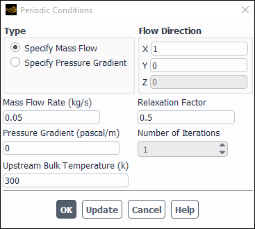
Controls
- Specify Mass Flow
enables the specification of the mass flow rate.
- Specify Pressure Gradient
enables the specification of the pressure gradient.
- Mass Flow Rate
specifies the mass flow rate. This item will not be available if you selected the Specify Pressure Gradient option.
Important: For axisymmetric problems, the mass flow rate is per
 radians.
 - Pressure Gradient
specifies the pressure gradient (
 in Equation 1–22 in the
Theory Guide).
in Equation 1–22 in the
Theory Guide).- Upstream Bulk Temperature
sets the inlet bulk temperature for periodic heat transfer calculations.
- Flow Direction
sets the direction of the periodic flow. The direction vector must be parallel to the periodic translation direction or its opposite.
- Relaxation Factor
sets the under-relaxation factor that controls convergence of the iteration process described in Setting Parameters for the Calculation of β for specified mass flow.
- Number of Iterations
sets the number of subiterations done on the correction of
 in the pressure correction equation for specified mass flow. See Setting Parameters for the Calculation of β for details.
- Update
updates the Pressure Gradient field with the current value.
The Perforated Walls dialog box opens when you click the Perforated Walls... in the Boundary Conditions task page. It allows you to set parameters that define perforated walls boundary conditions. See Perforated Wall Boundary Conditions for details.
(This dialog box is available only when the pressure-based solver is used; it is not available for the density-based solvers.)
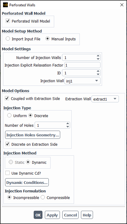
Controls
- Perforated Wall Model
enables the perforated wall model described in Perforated Wall Boundary Conditions.
- Model Setup Method
is where you can select an appropriate method for setting up the perforated wall model. The following parameters and options are available:
- Import Input Files
allows you to read an input file that contains the selections of model options and values of the model parameters. This option is useful for cases where hundreds or even thousands of perforated holes need to be defined.
- Manual Inputs
allows you to manually specify options and parameters for the perforated wall model. When this option is selected, the Perforated Walls dialog box expands to reveal relevant model inputs.
- Model Settings
is where you can specify:
- Number of Injection Walls
specifies the total number of injection walls. You will need to define boundary conditions for each wall separately.
- Injection Explicit Relaxation Factor
controls the update of the injection mass flow rate at each iteration. It is used to blend the injection mass flow rates calculated by Equation 7–131 (for incompressible flow) or Equation 7–132 (for compressible flow) at the current and previous iterations.
- ID
sets the ID number of the injection wall. This number must be between 1 and the value specified in Number of Injection Walls.
- Injection Wall
allows you to select the name of the injection wall.
- Model Options
is a group box that contains the following settings:
- Extraction Wall
allows you to select the extraction wall you want to couple with the injection wall.
- Injection Type
is where you can select Uniform or Discrete modeling approach. See Modeling Concept for more information about these two approaches.
For the Discrete injection type, you also need to specify the following:
- Number of Holes
sets the total number of perforated holes in the injection wall.
- Injection Holes Geometry...
opens the Injection Holes dialog box. See Setting Perforated Walls for detailed information about this dialog box.
- Discrete on Extraction Side
disabling this option allows you to model the uniform condition on the extraction side. This option is enabled by default.
- Injection Method
is where you can set the following:
- Dynamic Conditions...
opens the Dynamic Setup dialog box. See Setting Perforated Walls for detailed information about this dialog box.
- Injection Formulation
allows you to choose the injection formulation from the following options:
Incompressible: uses Equation 7–131 to calculate the injection mass flow rate at the hole exit.
Compressible: uses Equation 7–132 to calculate the injection mass flow rate at the hole exit.
- CHT Coupling
(cases with solid zone(s) only) when enabled, includes the effects of conjugate heat transfer between the solid walls and the injection flow. See Procedure for Manual Setup of Perforated Walls for more information about this option.