


When interpreting time-sequence data from a transient solution, it is often useful to look at the data’s spectral (frequency) attributes. For instance, you may want to determine the major vortex-shedding frequency from the time-history of the drag force on a body recorded during an Ansys Fluent simulation. Or, you may want to compute the spectral distribution of static pressure data recorded at a particular location on a body surface. Similarly, you may need to compute the spectral distribution of turbulent kinetic energy using data for fluctuating velocity components. To interpret some of these time dependent data, you need to perform Fourier transform analysis. In essence, the Fourier transform enables you to take any time dependent data and resolve it into an equivalent summation of sine and cosine waves.
Ansys Fluent enables you to analyze your time dependent data using the Fast Fourier Transform (FFT) algorithm. Information on using the FFT algorithm in Ansys Fluent is provided in the following sections:
The following limitations apply to Ansys Fluent’s FFT module:
The Ansys Fluent FFT module can only read inputs files in the following formats: Ansys Fluent report file, monitor, x-y file, Krichhoff model signal (
*.ark), and Ffowcs Williams and Hawkings model signal (*.ard).The Ansys Fluent FFT module assumes that the input data have been sampled at equal intervals and are consecutive (in the order of increasing time).
The lowest frequency that the FFT module can pick up is given by
 , where
  is the total sampling time. If the sampled sequence
contains frequencies lower than this, these frequencies will be aliased
into higher frequencies.
is the total sampling time. If the sampled sequence
contains frequencies lower than this, these frequencies will be aliased
into higher frequencies.The highest frequency that the FFT module can pick up is
 , where
  is the sampling
interval (or time step).
is the sampling
interval (or time step).
The discrete FFT algorithm is based on the assumption that the time-sequence data passed to the FFT corresponds to a single period of a periodically repeating signal. Since, in most situations, the first and the last data points will not coincide, the repeating signal implied in the assumption can often have a large discontinuity. The large discontinuity produces high-frequency components in the resulting Fourier modes, causing an aliasing error. You can condition the input signal before the transform by “windowing” it, in order to avoid this problem.
Suppose that we have  consecutive discrete (time-sequence) data sampled
with a constant interval,
consecutive discrete (time-sequence) data sampled
with a constant interval,  :
:
 | (40–2) |
Windowing is done by multiplying the original input data ( )
by a window function,
)
by a window function,  :
:
 | (40–3) |
Ansys Fluent offers four different window functions:
Hamming’s window:
 | (40–4) |
Hanning’s window:
 | (40–5) |
Bartlett’s window:
 | (40–6) |
Blackman’s window:
 | (40–7) |
These window functions preserve a large fraction ( ) of the original data, affecting only
  of the data on both ends.
The Fourier transform utility in Ansys Fluent enables you to
compute the Fourier transform of a signal,  , a real-valued
function, from a finite number of its sampled points.
, a real-valued
function, from a finite number of its sampled points.
For a periodic set of  sampled points,
  , the discrete Fourier transform [21] expresses the signal as a finite trigonometric
series:
, the discrete Fourier transform [21] expresses the signal as a finite trigonometric
series:
 | (40–8) |
where the series coefficients  are computed as
 | (40–9) |
Equation 40–8 and Equation 40–9 form a Fourier transform pair that enables us to determine one from the other.
Note that when we follow the convention of varying  from
from  to
to  in Equation 40–8 and Equation 40–9 instead of from
  to
to  , the range of index
  corresponds to positive
frequencies, and the range of index
corresponds to positive
frequencies, and the range of index  corresponds to negative
frequencies.
corresponds to negative
frequencies.  still corresponds to zero frequency.
For the actual calculation of the transforms, Ansys Fluent adopts
the so-called fast Fourier transform (FFT) algorithm, which significantly
reduces operation counts in comparison to the direct transform. Furthermore,
unlike most FFT algorithms in which the number of data should be a
power of 2, the FFT utility in Ansys Fluent employs a prime-factor
algorithm [161]. The number of data
points permissible in the prime-factor FFT algorithm is any products
of mutually prime factors from the set  , with a maximum value of
  . Thus, the prime-factor
FFT preserves the original data better than the conventional FFT.
. Thus, the prime-factor
FFT preserves the original data better than the conventional FFT.
Just prior to computing the transform, Ansys Fluent determines the largest permissible number of data points based on the prime factors, discarding the rest of the data. A list of these numbers is provided in Table 40.2: Numbers of Data Points Supported by the Prime-Factor FFT Algorithm.
Table 40.2: Numbers of Data Points Supported by the Prime-Factor FFT Algorithm
| 2 | 70 | 220 | 572 | 1386 | 3120 | 8580 | 34320 |
| 4 | 72 | 234 | 616 | 1430 | 3276 | 9240 | 36036 |
| 6 | 78 | 240 | 624 | 1456 | 3432 | 9360 | 40040 |
| 8 | 80 | 252 | 630 | 1540 | 3640 | 10010 | 48048 |
| 10 | 84 | 260 | 660 | 1560 | 3696 | 10296 | 51480 |
| 12 | 88 | 264 | 720 | 1584 | 3960 | 10920 | 55440 |
| 14 | 90 | 280 | 728 | 1638 | 4004 | 11088 | 60060 |
| 16 | 104 | 286 | 770 | 1680 | 4290 | 11440 | 65520 |
| 18 | 110 | 308 | 780 | 1716 | 4368 | 12012 | 72072 |
| 20 | 112 | 312 | 792 | 1820 | 4620 | 12870 | 80080 |
| 22 | 120 | 330 | 840 | 1848 | 4680 | 13104 | 90090 |
| 24 | 126 | 336 | 858 | 1872 | 5040 | 13860 | 102960 |
| 26 | 130 | 360 | 880 | 1980 | 5148 | 16016 | 120120 |
| 28 | 132 | 364 | 910 | 2002 | 5460 | 16380 | 144144 |
| 30 | 140 | 390 | 924 | 2184 | 5544 | 17160 | 180180 |
| 36 | 144 | 396 | 936 | 2288 | 5720 | 18018 | 240240 |
| 39 | 154 | 420 | 990 | 2310 | 6006 | 18480 | 360360 |
| 40 | 156 | 440 | 1008 | 2340 | 6160 | 20020 | 720720 |
| 42 | 168 | 462 | 1040 | 2520 | 6552 | 20592 | |
| 44 | 176 | 468 | 1092 | 2574 | 6864 | 21840 | |
| 48 | 180 | 504 | 1144 | 2640 | 6930 | 24024 | |
| 52 | 182 | 520 | 1170 | 2730 | 7280 | 25740 | |
| 56 | 198 | 528 | 1232 | 2772 | 7920 | 27720 | |
| 60 | 208 | 546 | 1260 | 2860 | 8008 | 30030 | |
| 66 | 210 | 560 | 1320 | 3080 | 8190 | 32760 |
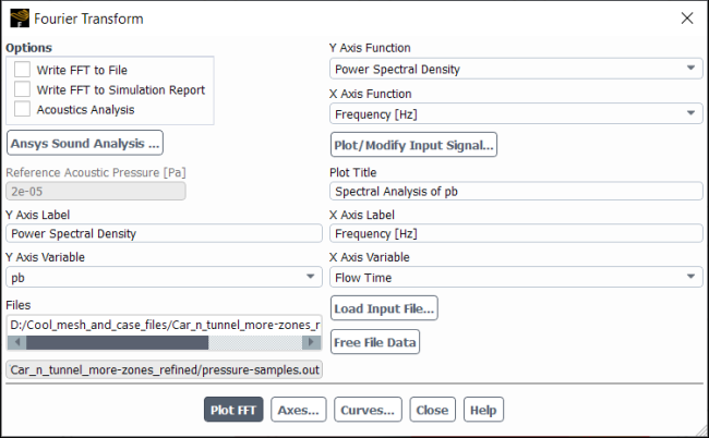
The Ansys Fluent FFT utility is available through the Fourier Transform Dialog Box (Figure 40.124: The Fourier Transform Dialog Box).
![]() Results →
Results → ![]() Plots →
Plots → ![]() FFT → Set Up...
FFT → Set Up...
Note: The threshold behavior of reverting to standard plotting from enhanced interactive plotting (Enhanced Interactive Plots) does not work for Fast Fourier Transform (FFT) plots.
FFT analysis requires an input signal data file consisting of time-sequence data. To load an input signal data file into the Fourier Transform Dialog Box, click . This displays The Select File Dialog Box where you can browse through your file directories and locate your data file containing your time-sequence data. To remove a file from the Files list, select it and then click .
If you computed acoustic signals “on the fly”, you have the option of processing signal data from a file or processing receiver data stored in memory. To analyze signal data from an existing input file, select Process File Data under Process Options and proceed as described above. To analyze receiver data stored in memory, select Process Receiver under Process Options and select the appropriate receiver in the Receiver list. If your model results include receiver signals for both the Ffowcs Williams – Hawkings model and the wave equation-based Kirchhoff model, the signals will be taken for the model which is currently active in your Fluent session.
Click Plot FFT to display the spectral analysis data and, if you have enabled Acoustics Analysis, to calculate the overall sound pressure level in dB based on the Reference Acoustic Pressure and display it in the console.
Note: You can specify the  axis and
  axis variables if your input report file contains multiple
report definitions.
axis variables if your input report file contains multiple
report definitions.
With the input signal data file loaded into the Fourier Transform Dialog Box, you may want to view a plot of the input signal and/or customize the data set in preparation for applying the FFT algorithm. To do so, click the Plot/Modify Input Signal button to open the Plot/Modify Input Signal Dialog Box (Figure 40.125: The Plot/Modify Input Signal Dialog Box).
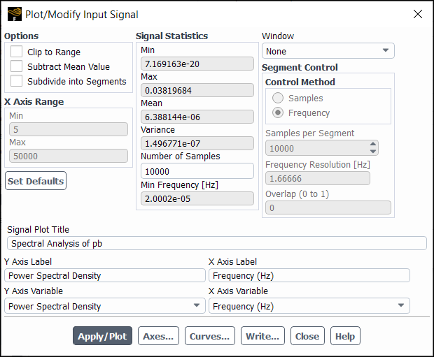
The Plot/Modify Input Signal Dialog Box allows you to analyze a portion of the input signal, view input Signal Statistics—Min, Max, Mean, Variance, total Number of Samples, and Min Frequency (that is, the finest possible frequency resolution)—and set title and label information for the input signal plot. Additionally, this dialog box allows you to enable and control the smoothing of the resulting spectrum by subdividing the input signal into multiple segments and averaging the segment-based spectra.
Note: You can specify the axis and axis variables if your input report file contains multiple
report definitions.
By default, the entire data set is analyzed. To analyze a portion of the input signal, enable
the Clip to Range option and specify the data range by
entering Min and Max values under
X Axis Range. To have the -axis quantities reduced by the Mean
value of the relevant signal property, enable the Subtract Mean
Value option.
The Set Defaults button will reset the original values for the Min and Max fields under X Axis Range and turn off the Clip to Range option.
For long broadband noise signals, the computed Fourier spectrum may display spurious fluctuations of amplitudes between the neighboring modes. In order to obtain a smooth spectrum, you can split the signal into multiple overlapping segments so that Ansys Fluent can apply the FFT algorithm on each segment and then average the resulting spectra. This procedure allows you to significantly suppress the spurious fluctuations at the cost of coarsening the frequency resolution of the spectrum. Note that the arithmetic averaging of spectra is performed for the squares of Fourier amplitudes, thus conserving the signal energy.
To use the smoothing procedure, enable the Subdivide
into Segments option and define the segment size and the
overlap of the subsequent segments in the Segment Control group box. Make a selection from the Control Method list to specify how you want to define the segment size: select Samples if you want to specify the number of Samples per Segment; select Frequency if you want to specify the desired Frequency Resolution  in Hertz units (the
segment length in seconds is then equal to
in Hertz units (the
segment length in seconds is then equal to  ). To
help determine a suitable segment size, you can use the Number of Samples and the Min Frequency information in the Signal Statistics group
box. Note that the final segment length is selected by Ansys Fluent to
adhere to the largest supported number of data samples (see Table 40.2: Numbers of Data Points Supported by the Prime-Factor FFT Algorithm). The actual signal length and
the number of segments will be displayed in the console when you plot
or write the Fourier spectrum. The number of segments depends on the Overlap of the subsequent segments, which is specified
regardless of which Control Method you select.
If you select a Window function (see Windowing for details), it is recommended
that you use an Overlap value of at least 0.125,
in order to cover the signal portion affected by the window function.
Generally, an Overlap value of 0.5 is recommended.
The exact number of samples that are in the overlapping region of
the segment can be determined from the segment hop size, which is
displayed in the console. The segment hop size is the distance (in
terms of samples) between the starting samples of any two adjacent
segments (that is, the shift from one segment to the next), and has
a minimum value of 1.
). To
help determine a suitable segment size, you can use the Number of Samples and the Min Frequency information in the Signal Statistics group
box. Note that the final segment length is selected by Ansys Fluent to
adhere to the largest supported number of data samples (see Table 40.2: Numbers of Data Points Supported by the Prime-Factor FFT Algorithm). The actual signal length and
the number of segments will be displayed in the console when you plot
or write the Fourier spectrum. The number of segments depends on the Overlap of the subsequent segments, which is specified
regardless of which Control Method you select.
If you select a Window function (see Windowing for details), it is recommended
that you use an Overlap value of at least 0.125,
in order to cover the signal portion affected by the window function.
Generally, an Overlap value of 0.5 is recommended.
The exact number of samples that are in the overlapping region of
the segment can be determined from the segment hop size, which is
displayed in the console. The segment hop size is the distance (in
terms of samples) between the starting samples of any two adjacent
segments (that is, the shift from one segment to the next), and has
a minimum value of 1.
The button will reset the segment control values and disable the Subdivide into Segments option.
To aid in the signal analysis, whether for the entire input signal or for a certain range of data, the Signal Statistics group box in the Plot/Modify Input Signal Dialog Box displays signal information such as the minimum, maximum, and average signal values, as well as the signal variance, total number of samples, and finest possible frequency resolution.
You can create a new title or edit the original title for the input signal plot by entering a text string in Signal Plot Title. Likewise, you can create a new axis label or edit the original axis label by entering a text string into either Y Axis Label or X Axis Label.
To apply any changes you have made in the Plot/Modify Input Signal Dialog Box and view a plot of the input signal, click .
In most practical applications with CFD data, you may want to find out how much power or energy is contained in a certain frequency range, but do not want to distinguish positive and negative frequency. In recognition of this, all the outputs from the FFT module in Ansys Fluent pertain to one-sided spectra for the range of positive frequency.
The Fourier Transform Dialog Box (Figure 40.124: The Fourier Transform Dialog Box) and Plot/Modify Input Signal Dialog Box (Figure 40.125: The Plot/Modify Input Signal Dialog Box) enable you to set several
different functions for the and  axes, apply different FFT windowing techniques,
and set various output options.
axes, apply different FFT windowing techniques,
and set various output options.
You can choose the  -axis function using the Y Axis Function drop-down list. Available options for the
  -axis functions are as follows.
Note that the functions related to acoustics (all of which are measured
in dB) are only available when the Acoustics Analysis option is enabled.
-axis functions are as follows.
Note that the functions related to acoustics (all of which are measured
in dB) are only available when the Acoustics Analysis option is enabled.
The definitions are provided for  , and include contributions from both elements
of a complex conjugate pair
, and include contributions from both elements
of a complex conjugate pair  and
and  -
- . Note that in Ansys Fluent, the value of
  is always an even number.
- Power Spectral Density
is the distribution of signal power in the frequency domain. Its value and units depend on the X Axis Function choice. For the detailed spectral representation with all resolved harmonics (that is, when X Axis Function is either Frequency, Strouhal Number, or Fourier Mode), the Power Spectral Density (
 ) has
units of the signal magnitude squared over the frequency (for example,
Pa2/Hz) and is defined for the frequency
) has
units of the signal magnitude squared over the frequency (for example,
Pa2/Hz) and is defined for the frequency  as
as
(40–10)
where
 is the frequency
step in the discrete spectrum, and the Fourier mode power
is the frequency
step in the discrete spectrum, and the Fourier mode power  is computed as
(40–11)
For the octave analysis (that is, when the X Axis Function is either Octave Band or 1/3-Octave Band), the Power Spectral Density has units of the signal magnitude squared (for example, Pa2), and is defined for the frequency band
 as
as 
(40–12)
where
 includes all of the Fourier modes belonging to the
band.
includes all of the Fourier modes belonging to the
band.- Magnitude
is the amplitude. For the detailed spectral representation with all resolved harmonics (that is, when X Axis Function is either Frequency, Strouhal Number, or Fourier Mode), the Magnitude (
 ) is defined for the frequency
  as
as
(40–13)
where
 is the mean signal value.
For the octave analysis (that is, when the X Axis Function is either Octave Band or 1/3-Octave Band), the Magnitude is defined for the frequency band
 as
as 
(40–14)
where
 is calculated according to Equation 40–12.
- Sound Pressure Level (dB)
is the decibel level. For either general or acoustic data, when the sampled data is pressure (for example, static pressure or sound pressure), the Sound Pressure Level (dB) (
 ) is calculated in decibel units using
(40–15)
where
 is
the Power Spectral Density for either a particular
Fourier mode or a particular frequency band (see Equation 40–10 and Equation 40–12).
is
the Power Spectral Density for either a particular
Fourier mode or a particular frequency band (see Equation 40–10 and Equation 40–12).  is the reference acoustic pressure,
with a default value of 2
is the reference acoustic pressure,
with a default value of 2  10-5 Pa; you
can revise this value, as described in Enabling the FW-H Acoustics Model.
10-5 Pa; you
can revise this value, as described in Enabling the FW-H Acoustics Model.- Sound Amplitude (dB)
is similar to the Sound Pressure Level (dB), and is a logarithmic conversion of the pressure signal Magnitude into decibel units. The Sound Amplitude (dB) (
 ) is calculated for either a Fourier mode
or a frequency band using
) is calculated for either a Fourier mode
or a frequency band using
(40–16)
- A-Weighted, Sound Pressure Level (dB A)
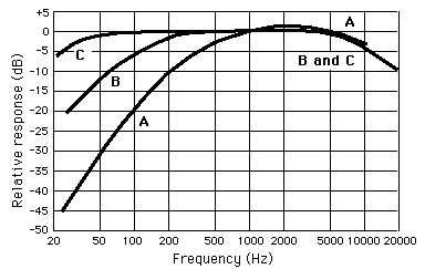
is the calculated sound pressure level weighted by the A-scale function to more closely approximate the frequency response of the human ear. A-Weighting is applied for loudness levels below 55 phons (55 dB at 1 kHz) and is the most commonly used weighting function. See Figure 40.126: A-, B-, and C-Weighting Functions for a graphical representation. This function is only available when the X Axis Function is either Octave Band or 1/3-Octave Band.
- B-Weighted, Sound Pressure Level (dB B)
is the calculated sound pressure level weighted by the B-scale function. B-Weighting is applied to loudness levels between 55 and 85 phons, though it is rarely used. See Figure 40.126: A-, B-, and C-Weighting Functions for a graphical representation. This function is only available when the X Axis Function is either Octave Band or 1/3-Octave Band.
- C-Weighted, Sound Pressure Level (dB C)
is the calculated sound pressure level weighted by the C-scale function. C-Weighting is applied for loudness levels above 85 phons and is commonly used for high-intensity sound such as traffic studies. See Figure 40.126: A-, B-, and C-Weighting Functions for a graphical representation. This function is only available when the X Axis Function is either Octave Band or 1/3-Octave Band.
Further graphical customizations for the  -axis are available by clicking
the Axes... button. For more information, see Modifying Axis Attributes.
-axis are available by clicking
the Axes... button. For more information, see Modifying Axis Attributes.
There are three options for the  -axis function you can choose
from in order to plot or write the detailed spectrum with all resolved
Fourier modes; these three options are related to the discrete frequencies
at which the Fourier coefficients are computed. There are also two
additional options available when the Acoustics Analysis option is enabled, which allow the octave and 1/3 octave band analysis.
You can apply specific analytic functions for the
-axis function you can choose
from in order to plot or write the detailed spectrum with all resolved
Fourier modes; these three options are related to the discrete frequencies
at which the Fourier coefficients are computed. There are also two
additional options available when the Acoustics Analysis option is enabled, which allow the octave and 1/3 octave band analysis.
You can apply specific analytic functions for the  -axis using the X Axis Function drop-down list.
Available options for the  -axis functions are as follows. The definitions are
provided for
-axis functions are as follows. The definitions are
provided for  , because the corresponding definitions for the
  -axis functions include contributions
from both elements of a complex conjugate pair
-axis functions include contributions
from both elements of a complex conjugate pair  and
and  -
- . Note that in Ansys Fluent, the value
of
. Note that in Ansys Fluent, the value
of  is always an even number.
- Frequency (Hz)
is defined as:

(40–17)
where
 is the number of data points used in the FFT.
- Strouhal Number
is the nondimensionalized version of the frequency defined in Equation 40–17 :

(40–18)
where
 and
and  are the reference length and velocity scales specified
in the Reference Values Task Page.
are the reference length and velocity scales specified
in the Reference Values Task Page.- Fourier Mode
is the index in Equation 40–8 and/or Equation 40–9, which represents the
 th term in the Fourier transform of the signal.
- Octave Band (Hz)
is a range of discrete frequency bands for different octaves within the threshold of hearing. The range of each octave band is double to that of the previous band (see Table 40.3: Octave Band Frequencies and Weightings).
- 1/3-Octave Band (Hz)
is a range of discrete frequency bands for different 1/3 octaves within the threshold of hearing.
Table 40.3: Octave Band Frequencies and Weightings
|
Lower Freq. (Hz) |
Center Freq. (Hz) |
Upper Freq. (Hz) |
dB A |
dB B |
dB C |
|---|---|---|---|---|---|
|
11 |
16 |
22 |
-56.7 |
-28.5 |
-8.5 |
|
22 |
31.5 |
45 |
-39.4 |
-17.1 |
-3.0 |
|
45 |
63 |
90 |
-26.2 |
-9.3 |
-0.8 |
|
90 |
125 |
180 |
-16.1 |
-4.2 |
-0.2 |
|
180 |
250 |
355 |
-8.6 |
-1.3 |
0.0 |
|
355 |
500 |
710 |
-3.2 |
-0.3 |
0.0 |
|
710 |
1000 |
1400 |
0.0 |
0.0 |
0.0 |
|
1400 |
2000 |
2800 |
1.2 |
-0.1 |
-0.2 |
|
2800 |
4000 |
5600 |
1.0 |
-0.7 |
-0.8 |
|
5600 |
8000 |
11200 |
-1.1 |
-2.9 |
-3.0 |
|
11200 |
16000 |
22400 |
-6.6 |
-8.4 |
-8.5 |
Further graphical customizations for the  -axis are available by clicking . For more information, see Modifying Axis Attributes.
You can write out the FFT data directly to a file by choosing the Write FFT to File option under Options in the Fourier Transform Dialog Box. Once the Write FFT to File option is selected, click to display a file selection dialog box where you can choose a file and/or a location to hold the FFT data. If Acoustics Analysis is selected, the overall sound pressure level will be calculated in dB (based on the Reference Acoustic Pressure) and displayed in the console at this time.
Further customizations for how the FFT data is displayed are available by clicking . For more information, see Modifying Curve Attributes.
You can use the various windowing techniques described in Windowing by selecting any of the Window options in the Plot/Modify Input Signal Dialog Box. By default, None is selected so that no windowing technique is applied.
You can assign a title for your FFT plot using the Plot Title text field.
You can also assign  -axis and
  -axis labels for your FFT plot using the Y Axis
Label and X Axis Label text fields,
respectively. By default,Ansys Fluent assigns the Y Axis
Label and the X Axis Label to the
particular selection of Y Axis Function and X
Axis Function.
-axis labels for your FFT plot using the Y Axis
Label and X Axis Label text fields,
respectively. By default,Ansys Fluent assigns the Y Axis
Label and the X Axis Label to the
particular selection of Y Axis Function and X
Axis Function.
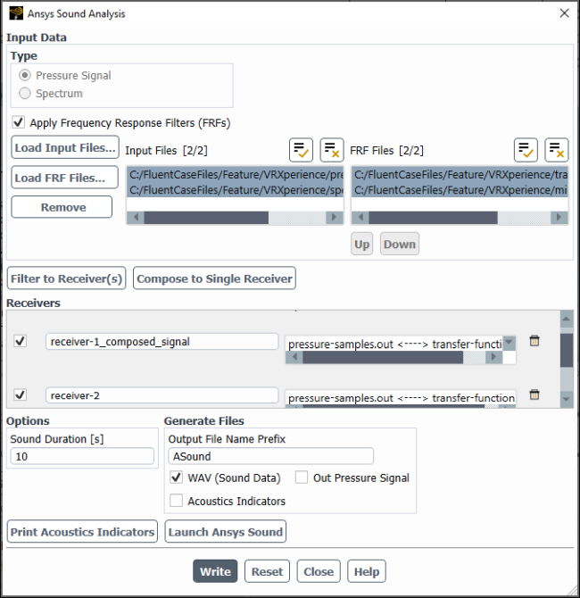
You can use the Ansys Sound Analysis dialog box to evaluate the acoustic indicators for one or more pressure signal or spectrum files. Using a frequency response filter (FRF) file, you can translate a pressure signal from one location to see the acoustic indicators at another location. You can also combine input files with FRFs to create a merged receiver for output at a single location. Output options include writing a WAV format sound file, output pressure signal, and/or acoustic indicator files. The WAV file can then be read into most suitable media players so you can hear the noise of the simulation results. The WAV file can also be read into Ansys Sound for listening and further analysis or combination with other simulation and measurement data.
To perform the acoustic analysis:
Open the Ansys Sound Analysis dialog box by clicking in Figure 40.124: The Fourier Transform Dialog Box.
Select the input file type.
Pressure Signal—an acoustic pressure file (two column file of time vs. pressure) that typically has an FMD file extension.
Example pressure signal file:
"pb" "Flow Time" "pb" ("Flow Time" "pb") 0.0005 -0.0031175 0.001 0.00365144 0.002 0.00954449 0.003 0.0145043 0.004 0.0184765 0.005 0.0214042 0.006 0.0232245 0.007 0.0238654 0.008 0.0232452 0.009 0.0212717 0.01 0.0178438Spectrum—an FFT output file (two column file of frequency vs. power spectral density).
Example spectrum file:
(title "Spectral Analysis of pb")
(labels "Frequency (Hz)" "Power Spectral Density")

((xy/key/label "pb")
5.0000000e+00	1.6515032e-05
1.0000000e+01	2.0448203e-06
1.5000000e+01	3.7586217e-06
2.0000000e+01	4.5504839e-06
2.5000000e+01	3.7905529e-06
3.0000000e+01	3.5729342e-06
3.5000000e+01	4.6056671e-06
4.0000000e+01	5.1608927e-06
4.5000000e+01	1.9510917e-06
5.0000000e+01	8.7493390e-06
5.5000000e+01	5.8902977e-05
6.0000000e+01	3.5942177e-04
6.5000000e+01	6.3120312e-04
(Optional) Enable Apply Frequency Response Filters (FRFs) to allow the loading of a frequency response filter (FRF) file.
Example FRF file:
AnsysSound_FRF 1
150    8.83959
200    31.1247
250    23.8472
300    5.65476
350    5.98757
400    29.6756
450    34.4814
500    41.3502
550    28.1577
600    19.6379
650    30.9932
700    19.093
750    22.9459
800    16.0768
850    30.0843
900    31.012
950    25.9581
1000    73.0306
Click to select the desired input file(s).
(If Apply Frequency Response Filters (FRFs) is enabled) Click Load FRF Files... to select the desired FRF file(s).
Select one or more Input Files and an equivalent number of FRF Files (if applicable).
Create one or more receivers:
Click to add one or more receivers that are mapped with one input file and one FRF file per receiver.
Click to combine the selected input files and corresponding FRF files into a single receiver.
Note that when you have multiple input files selected, the receivers are created assuming that the order of the FRF Files list matches the intended correspondence with the Input Files list. That is, the first input file will be paired with the first FRF file, the second input file will be paired with the second FRF file, and so on.
If you need to reorder the files for proper correspondence, you can click or to move the selected transfer function file in the list.
The Name of the receiver is used when you write the WAV file.
Specify the Sound Duration under Options.
Click , which computes the acoustic indicators on the active receiver(s) and prints them to the console.
Loudness [ISO 532B,Range -20 / + 140
										phones]
—The sensory scale of sound intensity. A sound perceived as twice as loud as another has double the loudness value in sones. Doubling a loudness value in sone (doubling the loudness sensation) corresponds to adding 10 phones to the loudness level. Refer to Loudness in the Ansys Sound: Analysis and Specification User's Guide for additional information.Sound Level [dB SPL,Range -20 / + 200 dB]—The equivalent continuous sound level. Its value is the average energy over time of the signal. Refer to Standard Levels in the Ansys Sound: Analysis and Specification User's Guide for additional information.Sound Level A-weighted [dBA SPL,Range -20 / + 200 dBA]—This is equivalent to the sound level, but with an A-weighting of the levels. Refer to Standard Levels in the Ansys Sound: Analysis and Specification User's Guide in the for additional information.Sharpness [DIN 45692, Range 0 / 10 acum]—An attribute that is related to the timbre of a sound. Sharpness is the subjective attribute describing the perception of the spectral balance of a sound. Sharpness is measured in "acum", which is defined as the sharpness of a narrow band of noise (one Bark) centered at one kHz at 60 dB SPL. Refer to Sharpness in the Ansys Sound: Analysis and Specification User's Guide for additional information.Tonality DIN 45681, [Range 0 / 100 dB] information is as follows:Mean difference DL (dB)Tonal Adjustment (dB)Number of tonesTonal adjustment Kt DIN 45981 (dB) is based on the DIN 45681:2005-03 standard. The standard describes a method to objectively determine the noise tonality and to determine the tonal adjustment for the evaluation of tonal emissions. Refer to DIN45681 in the Ansys Sound: Analysis and Specification User's Guide for additional information.
Articulation Index (ANSI
									S3.5-1969)
—Ranges from 0 (speech not intelligible) to (speech perfectly clear). Refer to Intelligibility in the Ansys Sound: Analysis and Specification User's Guide for additional information.
Note: The values of acoustic indicators (all the printed fields except Loudness) may vary when repeatedly computed. These differences are due to the Inverse Fast Fourier Transform (IFFT) that is performed, which uses random phases to generate a sound, from which the indicators are computed. The differences are small. Note that repeated experiments of the same phenomenon are unlikely to have exactly matching measurements, even though the samples sound the same. Refer to the point on the Hybrid/Automatic method in Methods for Sound Creation for additional information.
Select the types of files you want to save in the Generate Files group box.
WAV (Sound Data)—sound of the computed analysis that can be played using most media players.
Out Pressure Signal—output signal that can be read into Ansys Sound.
Acoustic Indicators—report of the acoustic indicators including sound level, frequency, and so on.
Click to save the specified receiver(s). Note, files are only written for the selected receivers (those with an enabled checkbox).
Two files are created for each receiver when you click ; a 32-bit file and a 16-bit file. The 16-bit WAV file is well suited for listening in any sound file player or being included in presentations. The 32-bit file contains the real physical values of the samples, but it is not always supported by all audio players (this can lead to distorted sound playback). Both files are fully supported in Ansys Sound SAS. It will keep the real physical values of each sample (with more precision in the 32-bit file, as the dynamic range is higher) and will not generate any artifacts while listening. Refer to File Formats for additional information on these files.
(Optional) Click to launch Ansys Sound: Analysis and Specification for further solution exploration (Welcome! in the Ansys Sound: Analysis and Specification User's Guide).
Ansys Sound: Analysis and Specification will launch with the selected receiver(s) open with the specified Sound Duration.