


This section describes how to use the Ansys Fluent's partially-premixed combustion model that is based on the non-premixed combustion model (Modeling Non-Premixed Combustion) and the premixed combustion model (Modeling Premixed Combustion). For information about the theory behind the partially premixed combustion model, see Partially Premixed Combustion in the Fluent Theory Guide.
Information about using the partially premixed combustion model is presented in the following sections:
The underlying theory, assumptions, and limitations of the non-premixed and premixed models apply directly to the partially premixed model. In particular, the single-mixture-fraction approach is limited to two inlet streams, which may be pure fuel, pure oxidizer, or a mixture of fuel and oxidizer. The two-mixture-fraction model extends the number of inlet streams to three, but incurs a major computational overhead. See Limitations of the Premixed Combustion Model for additional limitations.
The Flamelet Generated Manifold (FGM) model is limited to the c-Equation partially-premixed model.
The procedure for setting up and solving a partially premixed combustion problem combines parts of the non-premixed combustion setup and the premixed combustion setup. An outline of the procedure is provided in Setup and Solution Procedure, along with information about where to look in the non-premixed and premixed combustion sections for details. Inputs that are specific to the partially premixed combustion model are provided in this section.
Information is provided in the following sections:
- 20.3.2.1. Setup and Solution Procedure
- 20.3.2.2. Importing a Flamelet
- 20.3.2.3. Flamelet Generated Manifold
- 20.3.2.4. Calculating the Look-Up Tables
- 20.3.2.5. Standard Files for Flamelet Generated Manifold Modeling
- 20.3.2.6. Setting Premix Flame Propagation Parameters
- 20.3.2.7. Modifying the Unburnt Mixture Property Polynomials
- 20.3.2.8. Modeling Strained Laminar Flame Speed
- 20.3.2.9. Modeling In Cylinder Combustion
- 20.3.2.10. Postprocessing for FGM Scalar Transport Calculations
Read your mesh file into Ansys Fluent and set up any other models you plan to use in conjunction with the partially premixed combustion model (turbulence, radiation, and so on).
Enable the partially premixed combustion model.
Turn on the Partially Premixed Combustion model in the Species Model dialog box.
Note: Make sure a turbulence model (other than the Spalart-Allmaras model) is selected before selecting a combustion model.
 Setup → Models → Species
  Edit...
If you select the C Equation as the Premixed Model, then you have the choice of selecting one of the following State Relation models in the Chemistry tab: Chemical Equilibrim, Steady Diffusion Flamelet, Unsteady Diffusion Flamelet (for steady-state simulations starting from a converged Steady Diffusion Flamelet solution), or Flamelet Generated Manifold.
If you select the G Equation as the Premixed Model, then you have the choice of selecting one of the following State Relation models in the Chemistry tab: Chemical Equilibrim or Steady Diffusion Flamelet.
In the Chemistry tab of the Species Model dialog box, select the appropriate State Relation based on the type of partially premixed model you want to simulate. In Ansys Fluent, there are two types of partially premixed models, namely a thin-flamelet model (equilibrium and diffusion flamelet) and a finite-thickness flamelet model, which is a Flamelet Generated Manifold. You can refer to Non-Premixed Combustion in the Fluent Theory Guide to learn about diffusion flamelets or Partially Premixed Combustion Theory in the Fluent Theory Guide for FGMs. Also, you can refer to Overview in the Fluent Theory Guide for general information about the thin-flamelet and finite-thickness flamelet models.
If you select Flamelet Generated Manifold, you will also need to define whether the FGM is calculated from a premixed or a diffusion flamelet, as well as the Turbulence-Chemistry Interaction in the Premix tab. The available options (Finite-Rate and Turbulent Flame Speed) are discussed in FGM Turbulent Closure in the Fluent Theory Guide.
In the Flamelet tab, you can modify the Flamelet Parameters as described in Flamelet Generated Manifold.
Generate a PDF look-up table. The table parameters are defined in Calculating the Look-Up Tables.
Important: If Ansys Fluent warns you during the partially premixed properties calculation that any parameters are out of the range for the laminar flame speed function, you will need to modify the piecewise-linear points manually before saving the PDF file. See Modifying the Unburnt Mixture Property Polynomials for details. Also, the calculation of the thermal diffusivity uses the thermal conductivity in the Create/Edit Materials dialog box. More accurate thermal diffusivity polynomials can be obtained by editing the thermal conductivity in the Create/Edit Materials dialog box and then clicking in the Properties tab.
Define the physical properties for the unburnt material in the domain.
Setup →  Materials
Ansys Fluent will automatically select the prepdf-polynomial function for Laminar Flame Speed, indicating that the piecewise-linear polynomial function from the PDF look-up table will be used to compute the laminar flame speed. You may also choose to enter a constant value, use a user-defined function, metghalchi-keck-law, laminar-flame-speed-computed, or apply laminar-flame-speed-library instead of a piecewise-linear polynomial function. See Laminar Flame Speed in the Fluent Theory Guide and Defining Physical Properties for the Unburnt Mixture for information about setting the other properties for the unburnt material.
Set the values for the mean progress variable (
 ) and the mean mixture fraction
(
) and the mean mixture fraction
( ) and its variance (
 ) at flow inlets and
exits. (For problems that include a secondary stream, you will define
boundary conditions for the mean secondary partial fraction and its
variance as well.) Setup → Boundary Conditions
) at flow inlets and
exits. (For problems that include a secondary stream, you will define
boundary conditions for the mean secondary partial fraction and its
variance as well.) Setup → Boundary Conditions See Defining Non-Premixed Boundary Conditions for guidelines on setting mixture fraction and variance conditions, as well as thermal and velocity conditions at inlets.
Important: There are two ways to specify a premixed inlet boundary condition:
If you defined the fuel composition in the Boundary tab to be the premixed inlet species, then you should set
 and
and  in the boundary condition dialog
boxes.
in the boundary condition dialog
boxes.If you set the fuel composition to pure fuel in the Boundary tab, you will need to set the correct equivalence ratio (
 ) and
) and  at your premixed inlet boundary
condition.
at your premixed inlet boundary
condition.
For example, if the premixed inlet of methane and air is at an equivalence ratio of 0.3, you can
specify the mass fraction of the fuel composition of
 =
0.017,
=
0.017,  = 0.236, and
  = 0.747 in the Boundary tab
and
= 0.747 in the Boundary tab
and  = 1 and
  = 0 in the boundary condition dialog box.
specify the mass fraction of the fuel composition of
 =
1.0 in the Boundary tab and
=
1.0 in the Boundary tab and  = 0.017 and
  = 0 in the boundary condition
dialog box.
= 0 in the boundary condition
dialog box.Method (a) is preferred since it will have more points in the flame zone than method (b).
Initialize the value of the progress variable.
Solution →
Initialization → Patch...
See Initializing the Progress Variable for details.
You may be able to increase the robustness of the calculations by applying poor mesh numerics treatment to the cells that have an enthalpy value that is less than the minimum enthalpy defined in the PDF table. For details on how to easily apply such treatment, see Enabling Robust Numerics for Combustion with a PDF Table.
Solve the problem and perform postprocessing.
See Solving the Flow Problem for guidelines about setting solution parameters. (These guidelines are for non-premixed combustion calculations, but they are relevant for partially premixed as well.)
To import an existing flamelet file
Select the Import Flamelet option in the Chemistry tab of the Species Model dialog box.
Click the button. In The Select File Dialog Box, select the file to be read in to Ansys Fluent.
After you have completed this step, you can skip ahead to the Table tab of the Species Model dialog box (see Calculating the Look-Up Tables).
The Ansys Fluent Flamelet Generated Manifold (FGM) model has several advantages over the thin-flame equilibrium or diffusion steady flamelet models, such as the ability to model flame quenching due to dilution. The manifold can be modeled with either a Premixed Flamelet or a Diffusion Flamelet.
When Premixed Flamelet is selected as the Flamelet Type, you can select to solve the flamelets either in the Progress Variable Space or in the CHEMKIN Physical Space (Flamelet Solution Method group box). For more information about these methods, see Premixed FGMs in Reaction Progress Variable Space and Premixed FGMs in Physical Space in the Fluent Theory Guide.
When the Flamelet Generated Manifold state relation is selected in the Species Model dialog box (Chemistry tab), Ansys Fluent solves the reaction progress variable equation (Equation 8–113 in the Fluent Theory Guide). By default, Ansys Fluent uses the definition of the reaction progress variable as described in Premixed FGMs in Reaction Progress Variable Space in the Fluent Theory Guide. The default progress variable is a good and recommended choice for a wide range of hydrocarbon flames. However, if you want, you can adjust the definition of the progress variable as follows:
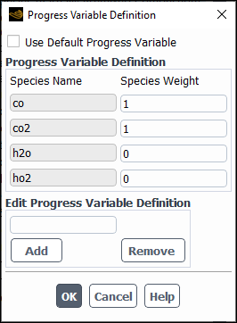
In the Species Model dialog box, click the Set Progress Variable... button (Boundary tab) to open the Progress Variable Definition dialog box. (See Figure 20.36: The Progress Variable Definition Dialog Box.)
The species used in the progress variable definition and their weights are displayed under Species Name and Species Weight, respectively.
Disable Use Default Progress Variable.
Edit the weight of the species as desired.
If you want to include a species in the progress variable composition, type its chemical formula (for example, h2o) under Edit Progress Variable Definition and click . The species will be added to the Species Name list.
Similarly, to remove a species from the Species Name list, type its chemical formula under Edit Progress Variable Definition and click .
To generate a flamelet file, go to the Flamelet tab of the Species Model dialog box (Figure 20.16: The Species Model Dialog Box (Flamelet Tab)), where you will enter values for parameters of the flamelet.
For premixed Flamelet Generated Manifolds, details about specifying the Scalar Dissipation at Stoichiometric Mixture Fraction can be found in Premixed FGMs in Reaction Progress Variable Space in the Fluent Theory Guide.
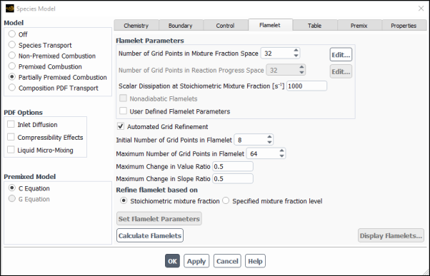
The Flamelet Parameters for premixed FGMs are as follows:
- Number of Grid Points in Mixture Fraction Space
specifies the number of mixture fraction grid points distributed between the oxidizer (
 ) and the fuel (
 ). Increased resolution will provide greater accuracy, but since
premixed flamelets are solved at all mixture fraction points, the flamelet
computation time will increase linearly with this input.
). Increased resolution will provide greater accuracy, but since
premixed flamelets are solved at all mixture fraction points, the flamelet
computation time will increase linearly with this input.- Number of Grid Points in Reaction Progress Space
specifies the number of reaction progress grid points distributed between unburnt (
 ) and burnt (
 ) states. Increased resolution will provide greater accuracy.
However, when the flamelets are generated in the Progress Variable
Space, the computation time and the required memory for the flamelets
calculation will increase with increasing resolution.
) states. Increased resolution will provide greater accuracy.
However, when the flamelets are generated in the Progress Variable
Space, the computation time and the required memory for the flamelets
calculation will increase with increasing resolution.- Scalar Dissipation at Stoichiometric Mixture Fraction
specifies the premixed flamelet strain rate. The default of 1000/s is an approximate value of the scalar dissipation of a freely propagating (unstrained) premixed flame at stoichiometric mixture fraction (unity equivalence ratio). This option is available only when the premixed FGM is generated in the Progress Variable Space.
- User Defined Flamelet Parameters
enables you to hook a user-defined function for scalar dissipation and mean mixture fraction (or progress variable) grid discretization
- Automated Grid Refinement
employs an adaptive algorithm, which inserts grid points so that the change of values, as well as the change of slopes, between successive grid points is less than user-specified tolerances. For information about this option, refer to Steady Diffusion Flamelet Automated Grid Refinement in the Theory Guide. Once this option is enabled, you can specify the following parameters:
- Initial Number of Grid Points in Flamelet
calculates a steady solution on a coarse grid, with a default of
 . See Equation 8–54 in the Theory Guide.
- Maximum Number of Grid Points in Flamelet
has a default of 64.
- Maximum Change in Value Ratio
has a default of 0.5 and is
 in Equation 8–28 in the Theory Guide.
- Maximum Change in Slope Ratio
has a default of 0.5 and is
 in Equation 8–29 in the Theory Guide.
- Refine flamelet based on
allows you to select either the Stoichiometric mixture fraction or Specified mixture fraction. For Specified mixture fraction, you must also specify a mixture fraction level at which the flamelet is solved during the grid refinement.
Note: When CHEMKIN Physical Space is selected as the Flamelet Solution Method for the Premixed Flamelet, the following default values are used for the Automated Grid Refinement parameters:
Initial Number of Grid Points in Flamelet = 12
Maximum Number of Grid Points in Flamelet =250
Maximum Change in Value Ratio = 0.5
Maximum Change in Slope Ratio = 0.1
Click to begin the premixed flamelet calculation.
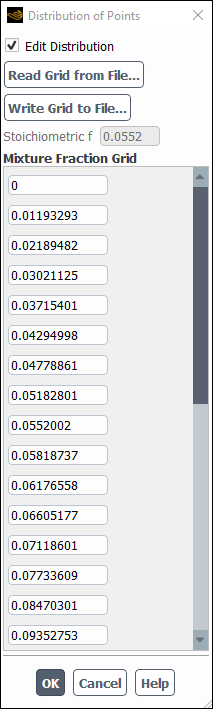
The default grid distribution for flamelet parameters is sufficient for most of the cases and should not be modified. However, in very specific cases, changing the grid distribution may improve accuracy. You can edit the grid distribution for the mixture fraction, and for with no automated grid refinement (AGR), for the reaction progress variable.
To edit the grid points, follow these steps:
Click the Edit... button next to the flamelet parameter for which you want to change the distribution grid points.
The Distribution of Points dialog box opens, showing the stoichiometric mixture fraction (in the Stoichiometric f field) and the default distribution of the grid points for the chosen flamelet parameter. In the example shown in Figure 20.38: The Distribution of Points Dialog Box, the grid point values are displayed in the Mixture Fraction Grid group box.
Enable Edit Distribution and modify the values of the grid points for the chosen flamelet parameter.
If you want to export the grid point data, use the button. The data will be saved in an ASCII file in the XY plot file format (see XY Plot File Format for details). Grid point pairs contain the point numbers and their values, separated by a space.
You can use the button to import a previously saved grid point file into your case.
Click .
Generating diffusion Flamelet Generated Manifolds is similar to generating Steady Diffusion Flamelets, as described in Calculating the Flamelets.
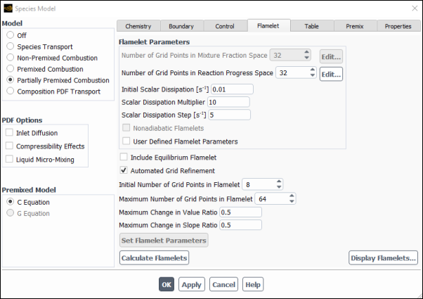
The parameters for the diffusion FGM flamelet are slightly different than those for the premixed FGM flamelet (see Premixed Flamelet Generated Manifolds for the definitions of the parameters). The additional diffusion FGM flamelet parameters are as follows:
- Initial Scalar Dissipation
is the scalar dissipation of the first flamelet in the library. This corresponds to
 in Equation 8–53 in the Fluent Theory Guide.
- Scalar Dissipation Multiplier
specifies the ratio of the scalar dissipation step in which successive flamelets are generated when the scalar dissipation is less than 1 s-1. This corresponds to
 for
for  < 1 in Equation 8–53 in the Theory Guide.
- Scalar Dissipation Step
specifies the interval between scalar dissipation values (in s-1) for which multiple flamelets will be calculated. This corresponds to
for  ≥ 1 in Equation 8–53 in the Theory Guide.
Note:The FGM model does not require the Maximum Number of Flamelets parameter. Instead, Ansys Fluent increases the scalar dissipation until the flamelet extinguishes. Hence, the Scalar Dissipation Step should be set at approximately one twentieth of the counterflow diffusion flamelet extinction strain rate, so that about twenty flamelets are calculated. The final, extinguishing unsteady diffusion flamelet is used to model the manifold between the unburnt state (
 ) and the last steady diffusion flamelet at the highest
scalar dissipation rate just before extinction.
) and the last steady diffusion flamelet at the highest
scalar dissipation rate just before extinction.Scalar Dissipation Multiplier and Scalar Dissipation Step are used to specify the interval of scalar dissipation for
 < 1 and
  ≥ 1, respectively. For example, for initial scalar
dissipation of 1e-3 s-1 with a Scalar
Dissipation Multiplier of 10, and a Scalar Dissipation
Step of 5, the flamelets will be generated with scalar
dissipations of 1e-3, 1e-2, 0.1, 1.0, 6, 11, 16, and so on.
≥ 1, respectively. For example, for initial scalar
dissipation of 1e-3 s-1 with a Scalar
Dissipation Multiplier of 10, and a Scalar Dissipation
Step of 5, the flamelets will be generated with scalar
dissipations of 1e-3, 1e-2, 0.1, 1.0, 6, 11, 16, and so on.
- Include Equilibrium Flamelet
determines how the progress variable (Equation 8–107 in the Fluent Theory Guide) is calculated. If this option is selected, Ansys Fluent will compute the progress variable using equilibrium. Otherwise, the progress variable will be computed using the solution of flamelet generated with initial scalar dissipation as a denominator in Equation 8–107 in the Fluent Theory Guide.
Note: The default grid distribution for flamelet parameters is sufficient for most of the cases and should not be modified. However, similar to the premixed FGM flamelet, in very specific cases, changing the grid distribution may improve accuracy. You can edit the grid distribution for the mixture fraction, and for cases with no AGR, for the reaction progress variable. The procedure for changing the grid points is described in Editing the Flamelet Grid Distribution.
When the following options are selected in the Species Model dialog box (Chemistry tab):
Premixed Flamelet as the Flamelet Type
Non-Adiabatic as the Energy Treatment
CHEMKIN Physical Space as the Flamelet Solution Method
you can select Nonadiabatic Flamelets in the Flamelet tab to generate the nonadiabatic flamelets as described in Nonadiabatic Flamelet Generated Manifold (FGM) in the Fluent Theory Guide.
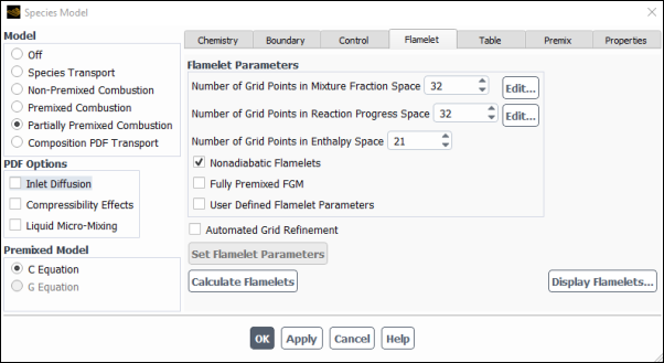
For nonadiablatic flamelet generation, you need to provide inputs in the Flamelet Parameters group box (Flamelet tab). Some parameters are the same as for premixed flamelet generated manifolds described in section Premixed Flamelet Generated Manifolds in the Ansys Fluent User's Guide. The additional parameters specific to nonadiabatic flamelets are as follows:
- Number of Grid Points in Enthalpy Space
specifies the number of enthalpy levels for which the flamelets will be generated. Ansys Fluent automatically distributes the enthalpy levels based on the reference fuel and oxidizer temperatures. A higher number of points provides the increased resolution in enthalpy space, but requires more computation time because each additional point in enthalpy space will generate a set of flamelets for entire mixture fraction space.
- Fully Premixed FGM
is an option to generate nonadiabatic flamelets only for one mixture fraction specified in the Mixture Fraction Value for Flamelet Generation entry field. This is useful for fully premixed CFD problems when the mixture fraction is constant, and flamelets are required only for a single mixture fraction. When this option is enabled, the Number of Grid Points in Mixture Fraction Space is automatically set to
1. Since the number of mixture fraction space is only1, this option is not only fast to generate the manifold, but it also produces flamelet and PDF files that are greatly reduced size.
Once you click Calculate Flamelets, Ansys Fluent will generate premixed nonadiabatic flamelets as described in Nonadiabatic Flamelet Generated Manifold (FGM) in the Fluent Theory Guide.
Ansys Fluent requires additional inputs that are used in the creation of the look-up tables. Several of these inputs control the number of discrete values for which the look-up tables will be computed. These parameters are input in the Table tab of the Species Model dialog box.
For the example of modeling a partially-premixed flame with either the premixed or the diffusion FGM model, the Table tab of the Species Model dialog box is shown in Figure 20.41: The Species Model Dialog Box: Table Tab with no Automated Grid Refinement when the Automated Grid Refinement (AGR) is disabled and Figure 20.42: The Species Model Dialog Box: Table Tab Displaying Automated Grid Refinement when the AGR is enabled.
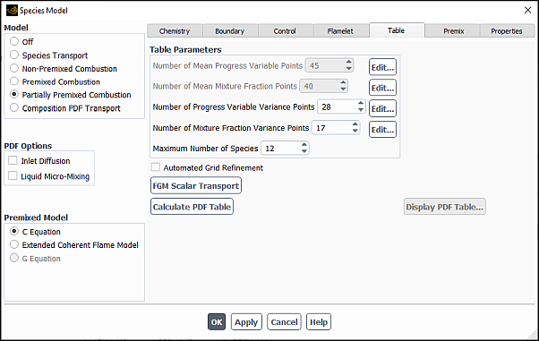
When the automated grid refinement is not selected, the look-up table parameters specific to the partial-premixed model are as follows:
- Number of Mean Progress Variable Points
is the number of discrete values of
 at which the look-up tables will be computed. This number is determined from the number of grid points in the flamelet.
- Number of Progress Variable Variance Points
is the number of discrete values of
 at which the look-up tables will be computed. Lower resolution is acceptable because the variation along the
  axis is, in general, not as steep as the variation along the
  axis of the look-up tables.
- Maximum Number of Species
is the maximum number of species that will be included in the look-up tables. The maximum number of species that can be included is 200. Ansys Fluent will automatically select the species with the largest mole fractions to include in the PDF table. Note that the PDF table values of density and specific heat are pre-calculated with all the species, and hence the convergence behavior of Ansys Fluent will not be affected by the input for the Maximum Number of Species. Hence, to keep table sizes small, you should set the Maximum Number of Species to only include the species that you are interested in postprocessing.
- Number of Mean Enthalpy Points
is the number of discrete values of enthalpy at which the look-up tables will be computed. This input is required only if you are modeling a non-adiabatic system. The number of points required will depend on the chemical system that you are considering, with more points required in high heat release systems (for example, hydrogen/oxygen flames).
- Minimum Temperature
is used to determine the lowest temperature for which the look-up tables are generated. Your input should correspond to the minimum temperature expected in the domain (for example, an inlet or wall temperature). The minimum temperature should be set 10–20 K below the minimum system temperature. This option is available only if you are modeling a non-adiabatic system.
Note: The default grid distribution for table parameters is sufficient for most of the cases and should not be modified. However, similar to flamelet parameters, the grid distribution can be modified when the AGR is disabled. Changing the grid distribution should be done only in very specific cases in order to improve accuracy. The procedure for changing the grid points is described in Editing the Flamelet Grid Distribution.
You can edit the grid point for the following table parameters:
Mean mixture fraction
Progress variable variance
Note that for the mean mixture fraction, you can enable the Use Flamelet Distribution option if you want to use the points of the grid distribution of the FGM flamelet.
Mean fraction variance
For the mean progress variable, you can view the grid distribution points, but you cannot edit them.
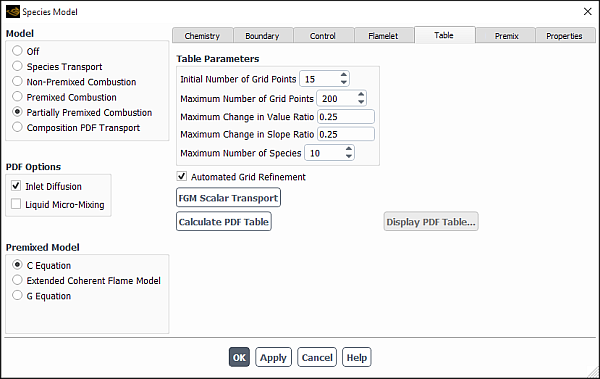
The look-up table parameters when Automated Grid Refinement is selected are as follows:
- Initial Number of Grid Points
specifies the number of grid points for the resolution of the mean mixture fraction, mixture fraction variance, and mean enthalpy (for non-adiabatic systems); and mean progress variable and progress variable variance (for FGM).
- Maximum Number of Grid Points
specifies the maximum number of grid points used for tabulation. The grid refinement procedure will stop inserting the points when either the change in value and slope between successive points is within tolerance or the maximum number of grid points are generated.
- Maximum Change in Value Ratio
specifies the maximum allowable change in value of table variables between successive grid points as specified by Equation 8–28 in the Theory Guide.
- Maximum Change in Slope Ratio
specifies the maximum change in the slope of table variables between successive grid points as specified by Equation 8–29 in the Theory Guide.
- Maximum Number of Species
is the maximum number of species stored in the lookup tables.
Note: Automated Grid Refinement is not available with two mixture fractions.
For the FGM model, you can solve additional transport equations for selected species mass fractions, called FGM scalars, as described in Scalar Transport with FGM Closure in the Fluent Theory Guide. To do so, click FGM Scalar Transport.
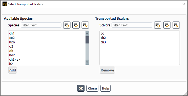
In the Select Transported Scalars dialog box that opens, select the FGM scalars as follows:
To add a species to the Transported Scalars list, select it in the Available Species multiple-selection list and click Add.
To remove a species from the Transported Scalars list back to the Available Species multiple-selection list, select it and click Remove.
For flow boundaries, you can specify the boundary conditions for the Scalar Mass Fractions for the selected transported scalars (in the Species tab of the corresponding boundary conditions dialog boxes).
During the solution run, Ansys Fluent will solve transport equations for the selected scalars and take their pre-computed averaged reaction rates from the PDF look-up table.
Note:
You must select the FGM transported scalars before calculating the PDF table. Once the table is calculated, you will no longer be able to modify the definition of the transported FGM scalars. In order to modify the FGM scalar definition after the PDF table has been calculated, you will need to re-import or regenerate the flamelets.
Since the scalar equations do not couple back into the flow equations or mixture properties, they could be solved in a postprocessing mode for a steady-state simulation, such as pollutant formation. In such cases, you could deselect FGM Scalar Transport from the Equations list solved by Ansys Fluent (in the Equations dialog box), and then select them again once the steady flow field has converged.
When you are satisfied with your inputs, click to generate the look-up tables.
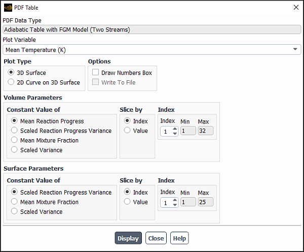
For the FGM model, the PDF table is four-dimensional for adiabatic cases and five-dimensional for non-adiabatic cases. For adiabatic PDF tables, the four independent variables are Mean mixture fraction, Mean reaction progress variable, Mixture fraction variance, and Progress variable variance. For non-adiabatic tables, the additional fifth independent variable is enthalpy. The FGM PDF tables can be post-processed using 2D curves and 3D surfaces by fixing two or more independent variables.
The procedure to display the lookup tables graphically is similar to that outlined in Postprocessing the Look-Up Table Data with additional steps as follows.
Adiabatic PDF Tables
3D surfaces:
Under Volume Parameters, select the discrete independent parameter to be held constant and fix it by specifying either a slice Index number or a Value. (For more information, see Postprocessing the Look-Up Table Data.)
In a similar manner, under Surface Parameters, select and fix the second discrete independent parameter and click Plot.
The resulting plot is a 3D surface of the selected Plot Variable as a function of the remaining two independent variables that have not been fixed.
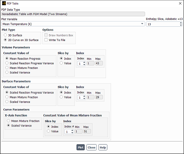
2D curves on 3D Surface:
Under Volume Parameters and Surface Parameters, fix discrete independent parameters as described above.
Under the Curve Parameters group box, select the X-Axis Function against which the plot variable will be displayed, fix the remaining discrete independent parameter using controls in the Constant Value of
Independent Parametergroup box, and click Plot.The resulting plot is a 2D curve of the selected Plot Variable as a function of the remaining independent variable that has not been fixed.
Non-Adiabatic PDF Tables
Fix the enthalpy slice level by specifying Enthalpy Slice.
For non-adiabatic PDF tables, heat loss/gain is the fifth independent variable, which is expressed as enthalpy levels. By default, the enthalpy level is fixed at the adiabatic level, which is displayed in the Enthalpy Slice, Adiabatic =
slice numberlabel, as shown in Figure 20.45: The PDF Table Dialog Box (Non-Adiabatic Case With FGM). Enthalpy slice numbers below the adiabatic slice number are associated with heat loss, while enthalpy slice numbers above the adiabatic slice number are associated with enthalpy gain.Depending on whether you want to display a 3D surface or a 2D Curve on 3D Surface, follow appropriate steps for Adiabatic PDF Tables described above.
A standard flamelet file format can be used to read and write FGM flamelets. The data structure for the standard flamelet file format is based on keywords that precede each data section. If any of the keywords in your flamelet data file do not match the supported keywords, you will have to manually edit the file and change the keywords to one of the supported types. (The Ansys Fluent flamelet filter is case-insensitive, so you need not worry about capitalization within the keywords.)
The following keywords are supported by the Ansys Fluent filter:
Header section:
HEADERMain body section:
BODYNumber of species:
NUMOFSPECIESNumber of grid points:
GRIDPOINTSPressure:
PRESSURETemperature:
TEMPERATUREandTEMPMass fraction:
MASSFRACTION-Mixture fraction:
ZMole fraction:
MOLEFRACTION-Scalar dissipation for premixed flamelet:
PREMIX_CHIReaction progress:
REACTION_PROGRESSReaction progress source term:
PREMIX_YCDOT
Note: Note that the FGM standard flamelet file format is identical for both premixed and diffusion flamelets. However, this format is different from the standard format for steady diffusion Laminar Flamelets, which is described in Calculating the Look-Up Tables.
A sample FGM file in the standard FGM format is provided below. Note that not all species are listed in this file.
HEADER
PREMIX_STOICH_SCADIS   1.000000E+01
Z         0.000000E+00
NUMOFSPECIES  53
GRIDPOINTS  32
STOICH_Z    5.520020e-02
PRESSURE  1.013250E+05
BODY
REACTION_PROGRESS
0.000000000E+00   5.625000000E-02   1.125000000E-01   1.687500000E-01   2.250000000E-01
2.812500000E-01   3.375000000E-01   3.937500000E-01   4.500000000E-01   5.062500000E-01
5.625000000E-01   6.187500000E-01   6.750000000E-01   7.312500000E-01   7.875000000E-01
8.437500000E-01   9.000000000E-01   9.508132748E-01   9.604275079E-01   9.668740305E-01
9.718608224E-01   9.759835686E-01   9.795270729E-01   9.826516818E-01   9.854574013E-01
9.880111737E-01   9.903602004E-01   9.925391181E-01   9.945741609E-01   9.964857158E-01
9.982899681E-01   1.000000000E+00
TEMPERATURE
3.000000000E+02   3.000000063E+02   3.000000126E+02   3.000000189E+02   3.000000251E+02
3.000000314E+02   3.000000377E+02   3.000000440E+02   3.000000503E+02   3.000000566E+02
3.000000628E+02   3.000000691E+02   3.000000754E+02   3.000000817E+02   3.000000880E+02
3.000000943E+02   3.000001006E+02   3.000001062E+02   3.000001073E+02   3.000001080E+02
3.000001086E+02   3.000001090E+02   3.000001094E+02   3.000001098E+02   3.000001101E+02
3.000001104E+02   3.000001107E+02   3.000001109E+02   3.000001111E+02   3.000001113E+02
3.000001115E+02   3.000001117E+02
massfraction-h2
0.000000000E+00   1.095241207E-53   2.190482414E-53   3.285723620E-53   4.380964827E-53
5.476206034E-53   6.571447241E-53   7.666688448E-53   8.761929655E-53   9.857170861E-53
1.095241207E-52   1.204765328E-52   1.314289448E-52   1.423813569E-52   1.533337690E-52
1.642861810E-52   1.752385931E-52   1.851324229E-52   1.870044058E-52   1.882596053E-52
1.892305813E-52   1.900333194E-52   1.907232735E-52   1.913316647E-52   1.918779651E-52
1.923752089E-52   1.928325868E-52   1.932568429E-52   1.936530852E-52   1.940252832E-52
1.943765883E-52   1.947095479E-52
 .  .   .    .    .
 .  .   .    .    .
PREMIX_YCDOT
0.000000000E+00   0.000000000E+00   0.000000000E+00   0.000000000E+00   0.000000000E+00
0.000000000E+00   0.000000000E+00   0.000000000E+00   0.000000000E+00   0.000000000E+00
0.000000000E+00   0.000000000E+00   0.000000000E+00   0.000000000E+00   0.000000000E+00
0.000000000E+00   0.000000000E+00   0.000000000E+00   0.000000000E+00   0.000000000E+00
0.000000000E+00   0.000000000E+00   0.000000000E+00   0.000000000E+00   0.000000000E+00
0.000000000E+00   0.000000000E+00   0.000000000E+00   0.000000000E+00   0.000000000E+00
0.000000000E+00   0.000000000E+00
Once the PDF look-up table is generated, you can specify the turbulent flame speed model options in the Premixed tab of the Species Model dialog box. For the FGM model, you can also specify the variance settings and select the turbulence-chemistry interaction model.
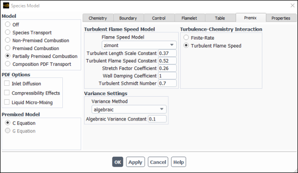
The following controls are available in the Turbulent Flamelet Speed Model group box.
- Flame speed Model
allows you to select the method to calculate turbulent flame speed as described in Turbulent Flame Speed Models in the Fluent Theory Guide.
If you selected zimont, you can adjust the Zimont model parameters as described in Modifying the Constants for the Zimont Flame Speed Model.
When the SBES turbulence model is used with the C Equation premixed model, you can also specify the following additional inputs:
- Turbulent Length Scale Constant (RANS)
is the modeling constant in the RANS region (
 in Equation 8–79 in the Theory
Guide).
in Equation 8–79 in the Theory
Guide).- Turbulent Flame Speed Constant (RANS)
is the modeling constant in the RANS region (
 in Equation 8–77 in the Theory Guide).
If you selected peters, you can adjust the Peters model parameters as described in Modifying the Constants for the Peters Flame Speed Model.
For the FGM model, you can adjust the following additional parameters:
- Turbulence-Chemistry Interaction
allows you to choose the method for modeling the source term in the progress variable equation (Equation 8–113 in the Fluent Theory Guide). The following methods are available:
Finite-Rate: Uses Equation 8–114 in the Fluent Theory Guide to calculate progress variable source terms from the PDF table.
Turbulent Flame Speed: Uses Equation 8–115 in the Fluent Theory Guide to calculate progress variable reaction source terms.
For more information about these models, see FGM Turbulent Closure in the Theory Guide.
- Variance Settings
contains the Variance Method drop-down list that allows you to choose between the following methods for calculating the progress variable variance:
transport equation (Equation 8–116 in the Fluent Theory Guide)
algebraic (Equation 8–117 in the Fluent Theory Guide)
(SBES only) hybrid (Equation 8–118 in the Fluent Theory Guide)
For the hybrid option, when applying Equation 8–118 in the Fluent Theory Guide, the algebraic model is used for
 and the transport equation model is used for
  .
. For the algebraic and hybrid options, you need to specify Algebraic Variance Constant (
 in Equation 8–117 in the Fluent Theory Guide).
It is recommended that you use the transport equation option for RANS, the algebraic option for LES, and the hybrid option for SBES.
After building the PDF table, Ansys Fluent automatically calculates the temperature,
density, heat capacity, and thermal diffusivity of the unburnt mixture as polynomial
functions of the mean mixture fraction,  (see Equation 8–127 in the Fluent Theory Guide). The laminar flame speed is automatically calculated as a piecewise-linear polynomial
function of
(see Equation 8–127 in the Fluent Theory Guide). The laminar flame speed is automatically calculated as a piecewise-linear polynomial
function of  .
.
However, as outlined in Partially Premixed Combustion Theory in the Fluent Theory Guide, the laminar flame speed depends on details of the chemical kinetics and molecular transport properties, and in the prepdf-polynomial method, it is not calculated directly. Instead, curve fits are made to flame speeds determined from detailed simulations [55]. These fits are limited to a range of fuels (H2, CH4, C2H2, C2H4, C2H6, and C3H8), air as the oxidizer, equivalence ratios of the lean limit through unity, unburnt temperatures from 298 K to 800 K, and pressures from 1 bar to 40 bars. If your parameters fall outside this range, Ansys Fluent will warn you when it computes the look-up table. In this case, you will need to modify the piecewise-linear points in the Properties tab of the Species Model dialog box (Figure 20.47: The Species Model Dialog Box (Properties Tab)) before you save the PDF file. If you selected the laminar-flame-speed-computed or laminar-flame-speed-library method, Ansys Fluent will automatically calculate the polynomial coefficient from computed flame speed or library. In both methods, the polynomial coefficient values of the laminar flame speed cannot be modified.
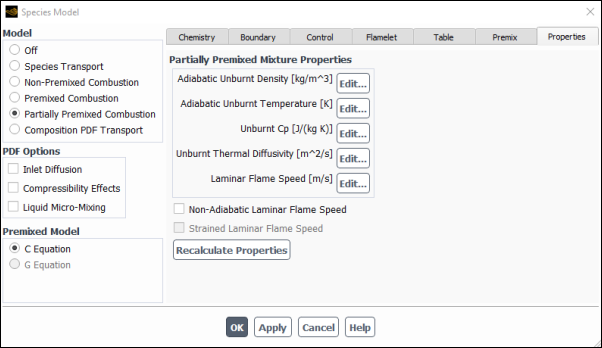
For each of the following
polynomial functions of the mean mixture fraction  in the Partially Premixed Mixture Properties group
box:
in the Partially Premixed Mixture Properties group
box:
Adiabatic Unburnt Density
Adiabatic Unburnt Temperature
Unburnt Cp
Unburnt Thermal Diffusivity
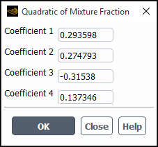
you can specify values for Coefficient 1, Coefficient 2, Coefficient 3, and Coefficient 4 (the polynomial coefficients in Equation 8–127 in the Fluent Theory Guide) in the Quadratic of Mixture Fraction dialog box, which opens when you click the button to the right of each property name. See Figure 20.48: The Quadratic of Mixture Fraction Dialog Box.
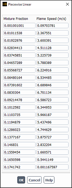
If you selected the prepdf-polynomial method for Laminar Flame Speed, you can also specify the piecewise-linear Mixture Fraction and its corresponding Flame Speed for 20 different points in the Piecewise Linear dialog box (Figure 20.49: The Piecewise Linear Dialog Box). The first set of values is the lower limit and the last set of values is the upper limit. Outside of either limit, the laminar flame speed is constant and equal to that limit. If you selected the laminar-flame-speed-library method, you can display the table, but you cannot modify the table values. To open the Piecewise Linear dialog box, click the button next to Laminar Flame Speed in the Properties tab.
Important: Note also that if you choose to use a user-defined function for the laminar flame speed in the Create/Edit Materials Dialog Box, the piecewise-linear fit becomes irrelevant.
If the secondary mixture fraction model is enabled, the unburnt properties are a function of both the mean and secondary mixture fractions. An additional column is added in the Piecewise Linear dialog box for the secondary mixture fraction unburnt polynomial coefficients.
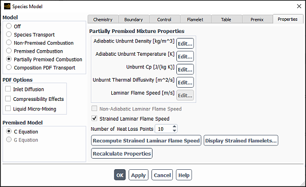
Note that the Non-Adiabatic Laminar Flame Speed option when enabled includes the non-adiabatic effects on the laminar flame speed by tabulating the laminar speeds in the PDF table. See Laminar Flame Speed in the Fluent Theory Guide.
For the Flamelet Generated Manifold (FGM) model with the turbulent flame speed model, you can model the strained laminar flame speed as follows:
Make sure Flamelet Generated Manifold is selected as the State Relation (Chemistry tab).
After calculating the flamelets and the PDF table (Flamelet and Table tabs), select Turbulent Flame Speed in the Turbulence-Chemistry Interaction group box and specify all relevant parameters (Premix tab).
In the Properties tab, enable Strained Laminar Flame Speed. This option appears only if you have imported a transport data file along with CHEMKIN mechanism and thermodynamic data files.
Click the button to generate strained flamelets for different mixture fraction points and strain rates.
If you are modeling non-adiabatic strained flame speed, then set the Number of Heat Loss Points to a value other than 1.
The heat loss points represent the different values of the heat loss parameter (Equation 8–139 in the Fluent Theory Guide). The default value of 1 corresponds to adiabatic strained flame speed. If you use more than one heat loss point in your simulation, the strained flame speed will be computed in increments of 0.05 of the heat loss parameter. For example, for three heat loss points, the strained non-adiabatic flame speed is computed for the heat loss parameters of 0, 0.05, and 0.1. For most applications, less than 10 heat loss points is sufficient.
See Strained Non-Adiabatic Flame Speed in the Fluent Theory Guide for more information.
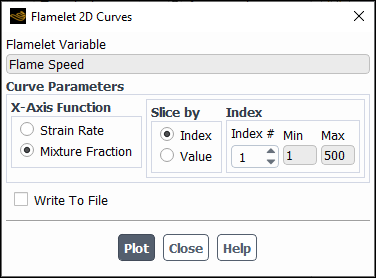
Once the flamelets are generated, you can display the flame speed as a function of the mixture fraction or strain rate using the button.
In the Flamelet 2D Curves dialog box that opens, Flame Speed appears as Flamelet Variable.
Specify the X-Axis Function against which the plot variable will be displayed by selecting Strain Rate or Mixture Fraction. The variable that is not selected will be held constant.
Specify the type of discretization (that is, how the flamelet data will be sliced) for the variable that is being held constant.
If you selected Index under Slice by, specify the discretization Index of the variable that is being held constant. The range of integer values that you are allowed to choose from is displayed under Min and Max, and is equivalent to the number of points used in postprocessing the flamelet data.
If you selected Value under Slice by, specify the numerical Value of the variable that is being held constant. The range of values that you can specify is displayed under Min and Max.
Click Plot.
Note that you can write flamelet table results to a file by using the Write to File option.
For more information about this model, refer to Strained Laminar Flame Speed in the Fluent Theory Guide.
Each of the partially premixed combustion models may be used for modeling in cylinder combustion. When modeling more than one cycle of such engines, you may choose to model trapped combustion products and exhaust gas recirculation (EGR) using the inert species model (see Setting Up the Inert Model). A Dynamic Mesh Event has also been provided for calculating the inert composition, converting burnt gases to inert and resetting the combustion process ready for the next cycle (see Resetting Inert EGR and Resetting Inert EGR).
In the case of the G-Equation model, this is the only way to automatically model multiple in cylinder combustion cycles and take into account trapped burnt gases remaining in the cylinder from one cycle to the next.
Ansys Fluent provides additional reporting options when you use the FGM Scalar Transport option for solving transport equations for the FGM scalars selected in the Select Transported Scalars dialog box. Quantities for reporting scalar mass fractions of the FGM scalars are contained in the Premixed Combustion… category the postprocessing dialog boxes.