


For background information about the Eulerian model and the limitations that apply, refer to Overview of the Eulerian Model in the Theory Guide.
For additional information, see the following sections:
- 26.5.1. Additional Guidelines for Eulerian Multiphase Simulations
- 26.5.2. Defining the Phases for the Eulerian Model
- 26.5.3. Modeling Turbulence
- 26.5.4. Including Heat Transfer Effects
- 26.5.5. Using an Algebraic Interfacial Area Model
- 26.5.6. Using the Algebraic Interfacial Area Density (AIAD) Model
- 26.5.7. Using the Generalized Two Phase Flow (GENTOP) Model
- 26.5.8. Including the Dense Discrete Phase Model
- 26.5.9. Including the Boiling Model
- 26.5.10. Setting Up Polydisperse Boiling
- 26.5.11. Including the Multi-Fluid VOF Model
Once you have determined that the Eulerian multiphase model is appropriate for your problem (as described in Choosing a General Multiphase Model in the Theory Guide), you should consider the computational effort required to solve your multiphase problem. The required computational effort depends strongly on the number of transport equations being solved and the degree of coupling. For the Eulerian multiphase model, which has a large number of highly coupled transport equations, computational expense will be high. Before setting up your problem, try to reduce the problem statement to the simplest form possible.
Instead of trying to solve your multiphase flow in all of its complexity on your first solution attempt, you can start with simple approximations and work your way up to the final form of the problem definition. Some suggestions for simplifying a multiphase flow problem are listed below:
Use a hexahedral or quadrilateral mesh (instead of a tetrahedral or triangular mesh).
Reduce the number of phases.
You may find that even a very simple approximation will provide you with useful information about your problem.
See Eulerian Model and Setting Solution Limits for more solution strategies for Eulerian multiphase calculations.
Instructions for specifying the necessary information for the primary and secondary phases and their interaction for an Eulerian multiphase calculation are provided below.
The procedure for defining the primary phase in an Eulerian multiphase calculation is the same as for a VOF calculation. See Defining the Primary Phase for details.
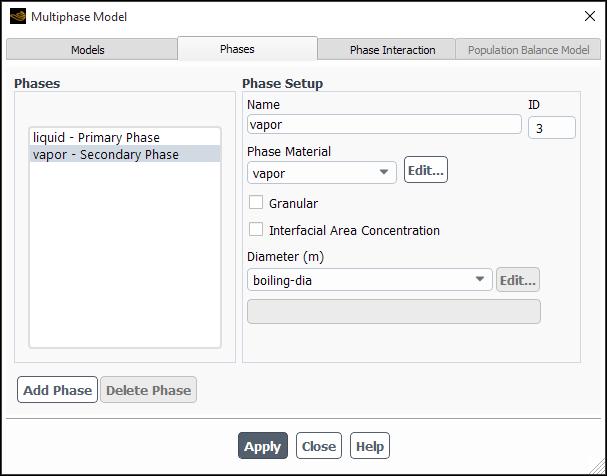
To define a non-granular (that is, liquid or vapor) secondary phase in an Eulerian multiphase calculation, go to the Phases tab in the Multiphase Model dialog box and perform the following steps:
Select the phase (for example, phase-2) in the Phases list.
In the Phase Setup group box, enter a Name for the phase (for example,
vapor).Specify which material the phase contains by choosing the appropriate material in the Phase Material drop-down list.
Define the material properties for the Phase Material, following the same procedure you used to set the material properties for the primary phase (see Defining the Primary Phase).
Specify the Diameter of the bubbles or droplets of this phase. You can specify a constant value, or use a user-defined function. See the Fluent Customization Manual for details about user-defined functions.
Click .
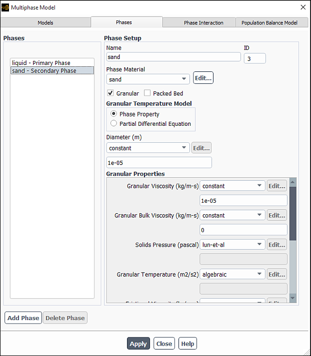
To define a granular (that is, particulate) secondary phase in an Eulerian multiphase calculation, go to the Phases tab in the Multiphase Model dialog box and perform the following steps::
Select the phase (for example, phase-2) in the Phases list.
In the Phase Setup group box, enter a Name for the phase (for example,
sand).Specify which material the phase contains by choosing the appropriate material in the Phase Material drop-down list.
Define the material properties for the Phase Material, following the same procedure you used to set the material properties for the primary phase (see Defining the Primary Phase). For a granular phase (which must be placed in the fluid materials category, as mentioned in Steps for Using a Multiphase Model), you need to specify only the density; you can ignore the values for the other properties, since they will not be used.
Important: Note that all properties for granular flows can be defined by user-defined functions (UDFs).
See the Fluent Customization Manual for details about user-defined functions.
Enable the Granular option.
(optional) Enable the Packed Bed option if you want to freeze the velocity field for the granular phase. Note that when you select the packed bed option for a phase, you should also use the fixed velocity option with a value of zero for all velocity components for all interior cell zones for that phase. Using fixed velocity in radial direction as a constant value (other than zero) does not ensure continuity. With the fixed velocity option, both velocity and pressure are fixed in a zone. Since face area in the radial direction is a function of radial distance from the axis, it will result in a mass conservation problem due to flux imbalance.
Using zero fixed velocity in the radial direction does not cause any problems related to mass conservation.
Specify the Granular Temperature Model. Choose either the default Phase Property option or the Partial Differential Equation option. See Granular Temperature in the Theory Guide for details.
Specifies the Diameter of the particles. You can select constant in the drop-down list and specify a constant value, or select user-defined to use a user-defined function. See the Fluent Customization Manual for details about user-defined functions.
In the Granular Properties group box, specify the following properties of the particles of this phase:
- Granular Viscosity
specifies the method for computing the kinetic (
 ) and collisional (
 ) components of the granular viscosity (Equation 14–362 in the Fluent Theory Guide). Selecting constant,
syamlal-obrien (Equation 14–364), or
gidaspow (Equation 14–365) will use these
expressions for the kinetic portion of the viscosity and will calculate the
collisional portion of the viscosity from Equation 14–363 in the Fluent Theory Guide. Alternatively, you can
select user-defined to use a user-defined function. Note
that if you select user-defined, your user-defined function
must include both the kinetic portion and the collisional portion of the
viscosity in the value it returns.
) components of the granular viscosity (Equation 14–362 in the Fluent Theory Guide). Selecting constant,
syamlal-obrien (Equation 14–364), or
gidaspow (Equation 14–365) will use these
expressions for the kinetic portion of the viscosity and will calculate the
collisional portion of the viscosity from Equation 14–363 in the Fluent Theory Guide. Alternatively, you can
select user-defined to use a user-defined function. Note
that if you select user-defined, your user-defined function
must include both the kinetic portion and the collisional portion of the
viscosity in the value it returns.
Note: If filtered is selected for Drag Coefficient, then Granular Viscosity is set automatically to filtered. The granular viscosity will be calculated as described in The Filtered Two-Fluid Model in the Fluent Theory Guide.
- Granular Bulk Viscosity
specifies the solids bulk viscosity (
 in Equation 14–195 in the Theory Guide). You can select
constant (the default) in the drop-down list and specify
a constant value, select lun-et-al to compute the value
using Equation 14–366 in the Theory Guide, or
select user-defined to use a user-defined function.
in Equation 14–195 in the Theory Guide). You can select
constant (the default) in the drop-down list and specify
a constant value, select lun-et-al to compute the value
using Equation 14–366 in the Theory Guide, or
select user-defined to use a user-defined function.Note: If filtered is selected for Drag Coefficient, then Granular Bulk Viscosity is set to zero automatically.
- Frictional Viscosity
specifies a shear viscosity based on the viscous-plastic flow (
 in Equation 14–362 in the Theory Guide). By default, the
frictional viscosity is neglected, as indicated by the default selection of
none in the drop-down list. If you want to include the
frictional viscosity, you can select constant and specify a
constant value, select schaeffer to compute the value using
Equation 14–367
in the Theory Guide, or
select user-defined to use a user-defined function.
in Equation 14–362 in the Theory Guide). By default, the
frictional viscosity is neglected, as indicated by the default selection of
none in the drop-down list. If you want to include the
frictional viscosity, you can select constant and specify a
constant value, select schaeffer to compute the value using
Equation 14–367
in the Theory Guide, or
select user-defined to use a user-defined function.- Angle of Internal Friction
specifies a constant value for the angle
 used in Schaeffer’s expression for frictional viscosity
(Equation 14–367 in the Theory Guide).
This parameter is relevant only if you have selected
schaeffer or user-defined for the
Frictional Viscosity.
used in Schaeffer’s expression for frictional viscosity
(Equation 14–367 in the Theory Guide).
This parameter is relevant only if you have selected
schaeffer or user-defined for the
Frictional Viscosity.- Frictional Pressure
specifies the pressure gradient term,
 , in the granular-phase momentum equation. Choose
none to exclude frictional pressure from your
calculation, johnson-et-al to apply Equation 14–371 in the Theory Guide,
syamlal-obrien to apply Equation 14–268 in the Theory Guide, based-ktgf,
where the frictional pressure is defined by the kinetic theory [38]. The solids pressure tends to a large value near the
packing limit, depending on the model selected for the radial distribution
function. You must hook a user-defined function when selecting the
user-defined option. See the Fluent Customization Manual for information on hooking a UDF.
, in the granular-phase momentum equation. Choose
none to exclude frictional pressure from your
calculation, johnson-et-al to apply Equation 14–371 in the Theory Guide,
syamlal-obrien to apply Equation 14–268 in the Theory Guide, based-ktgf,
where the frictional pressure is defined by the kinetic theory [38]. The solids pressure tends to a large value near the
packing limit, depending on the model selected for the radial distribution
function. You must hook a user-defined function when selecting the
user-defined option. See the Fluent Customization Manual for information on hooking a UDF.- Frictional Modulus
is defined as

(26–20)
with
 , which is the derived option. You can
also specify a user-defined function for the frictional
modulus.
, which is the derived option. You can
also specify a user-defined function for the frictional
modulus.- Friction Packing Limit
specifies a threshold volume fraction at which the frictional regime becomes dominant. The default value is 0.61.
- Granular Conductivity
specifies the solids granular conductivity (
 in Equation 14–374 in the Theory Guide). You can select
syamlal-obrien to compute the value using Equation 14–375 in the Theory Guide,
select gidaspow to compute the value using Equation 14–376 in the Theory Guide, or
select user-defined to use a user-defined function. Note
that in the algebraic model, shown in Figure 26.57: The Multiphase Model Dialog Box for a Granular Phase
(Phases Tab), the granular conductivity
is not required in the computation of the granular temperature. This has been
obtained by neglecting convection and diffusion in the transport equation,
Equation 14–374 in the
Theory Guide [157].
in Equation 14–374 in the Theory Guide). You can select
syamlal-obrien to compute the value using Equation 14–375 in the Theory Guide,
select gidaspow to compute the value using Equation 14–376 in the Theory Guide, or
select user-defined to use a user-defined function. Note
that in the algebraic model, shown in Figure 26.57: The Multiphase Model Dialog Box for a Granular Phase
(Phases Tab), the granular conductivity
is not required in the computation of the granular temperature. This has been
obtained by neglecting convection and diffusion in the transport equation,
Equation 14–374 in the
Theory Guide [157].- Granular Temperature
specifies temperature for the solids phase and is proportional to the kinetic energy of the random motion of the particles. Choose the algebraic, constant, dpm-averaged, or user-defined option.
Note:The dpm-averaged method is only available when using the Dense Discrete Phase Model (DDPM).
If filtered is selected for Drag Coefficient, then Granular Temperature is set automatically to zero.
- Solids Pressure
specifies the pressure gradient term,
 , in the granular-phase momentum equation. Choose either the
lun-et-al, the syamlal-obrien, the
ma-ahmadi, none, or a
user-defined option.
, in the granular-phase momentum equation. Choose either the
lun-et-al, the syamlal-obrien, the
ma-ahmadi, none, or a
user-defined option.Note: If filtered is selected for Drag Coefficient, then Solids Pressure is set automatically to filtered. The solid pressure will be calculated as described in The Filtered Two-Fluid Model in the Fluent Theory Guide.
- Radial Distribution
specifies a correction factor that modifies the probability of collisions between grains when the solid granular phase becomes dense. Choose either the lun-et-al, the syamlal-obrien, the ma-ahmadi, the arastoopour, or a user-defined option.
Note: If filtered is selected for Drag Coefficient, then Radial Distribution is set automatically to filtered. In the simulation, the radial distribution will be set to zero since the filtered two-fluid model is not based on kinetic theory.
- Elasticity Modulus
is defined as

(26–21)
with
 .
.- Packing Limit
specifies the maximum volume fraction for the granular phase. For monodispersed spheres, the packing limit is about 0.63, which is the default value in Ansys Fluent. In polydispersed cases, however, smaller spheres can fill the small gaps between larger spheres, so you may need to increase the maximum packing limit.
Click .
When using the Eulerian multiphase model, you can choose to solve a transport equation for the interfacial area, which allows for a distribution of secondary phase diameter, or you can use an algebraic model to compute the interfacial area from a specified diameter. To use an algebraic model, refer to Using an Algebraic Interfacial Area Model. To solve the transport equation (Interfacial Area Concentration in the Fluent Theory Guide), perform the following steps:
In the Multiphase Model dialog box, go to the Phase Interaction > Interfacial Area tab.
Select the phase (for example, phase-2) in the Phases list.
In the Phase Setup group box, enter a Name for the phase.
Specify which material the phase contains by choosing the appropriate material in the Phase Material drop-down list.
Define the material properties for the Phase Material.
Enable the Interfacial Area Concentration option. Make sure the Granular option is disabled for the Interfacial Area Concentration option to be visible in the interface.
Specify the Diameter of the particles or bubbles. You can select constant in the drop-down list and specify a constant value, or select user-defined to use a user-defined function. See the Fluent Customization Manual for details about user-defined functions. The Diameter recommended setting is sauter-mean, allowing for the effects of the interfacial area concentration values to be considered for mass, momentum and heat transfer across the interface between phases.
In the Interfacial Area Concentration Properties group box, specify the following properties of the particles of this phase:
- Coalescence Kernel and Breakage Kernel
allows you to specify the coalescence and breakage kernels. You can select none, constant, hibiki-ishii, ishii-kim, yao-morel, or user-defined. The three options, hibiki-ishii, ishii-kim and yao-morel are described in detail in Interfacial Area Concentration in the Theory Guide.
In addition to specifying the hibiki-ishii, ishii-kim, and yao-morel as the coalescence and breakage kernels, you can also tune the properties of the three models by using the
/define/phases/iac-expert/hibiki-ishii-model,/define/phases/iac-expert/ishii-kim-model, and/define/phases/iac-expert/yao-morel-modeltext commands.For each of the three models you can specify the parameters listed in Table 26.13: Parameters for the Coalescence and Breakage Kernels
Table 26.13: Parameters for the Coalescence and Breakage Kernels
Hibiki-Ishii Model Ishii-Kim Model Yao-Morel Model Coefficient Gamma_cCoefficient CrcCoefficient K_c1Coefficient K_cCoefficient CweCoefficient K_c3Coefficient Gamma_bCoefficient CCoefficient K_b1Coefficient K_bCoefficient Ctialpha_maxalpha_maxalpha_max
These values are discussed in greater detail in Interfacial Area Concentration in the Theory Guide.
- Nucleation Rate
is a source term for the interfacial area concentration that models the rate of formation of the dispersed phase. You can choose from constant or user-defined. If the Boiling Model option is enabled, you can also select yao-morel. The yao-morel option is described in Yao-Morel Model in the Theory Guide.
- Critical Weber Number
will need to be specified if you selected ishii-kim or yao-morel for the Breakage Kernel.
- Dissipation Function
gives you the option to choose the formula which calculates the dissipation rate used in the hibiki-ishii and ishii-kim models. You can choose amongst constant, wu-ishii-kim, fluent-ke, and user-defined for the dissipation function.
The wu-ishii-kim option uses a simple algebraic correlation for
 :
:
(26–22)
where

and

where
 ,
,  ,
,  , and
, and  are the mixture density, mixture velocity, mixture molecular
viscosity, and hydraulic diameter of the flow path.
are the mixture density, mixture velocity, mixture molecular
viscosity, and hydraulic diameter of the flow path.When you select the wu-ishii-kim model, you will set an additional input for Hydraulic Diameter.
- Hydraulic Diameter
is the value used in Equation 26–22, should you use the wu-ishii-kim formulation.
- Min/Max Diameter
allow you to specify the minimum and maximum diameters of the secondary phase to which the interfacial area concentration model is applied, preventing some computing anomalies to spread beyond control.
Click Apply.
Note: When solving a steady-state problem, the preferred setting for the
Under-Relaxation Factor is 1.0, as the interfacial area equation
for the boiling models is currently under-relaxed using a locally defined pseudo time
step. If you want extra explicit under-relaxation, you may set the value of the
Under-Relaxation Factor to less than one, this may be done only in
case of serious convergence problems with the interfacial area transport equation. To
improve convergence you can switch to a pseudo time step for the interfacial area
concentration only, using the
define/phases/iac-expert/iac-pseudo-time-step text command and
set the local pseudo time step to less than 1.
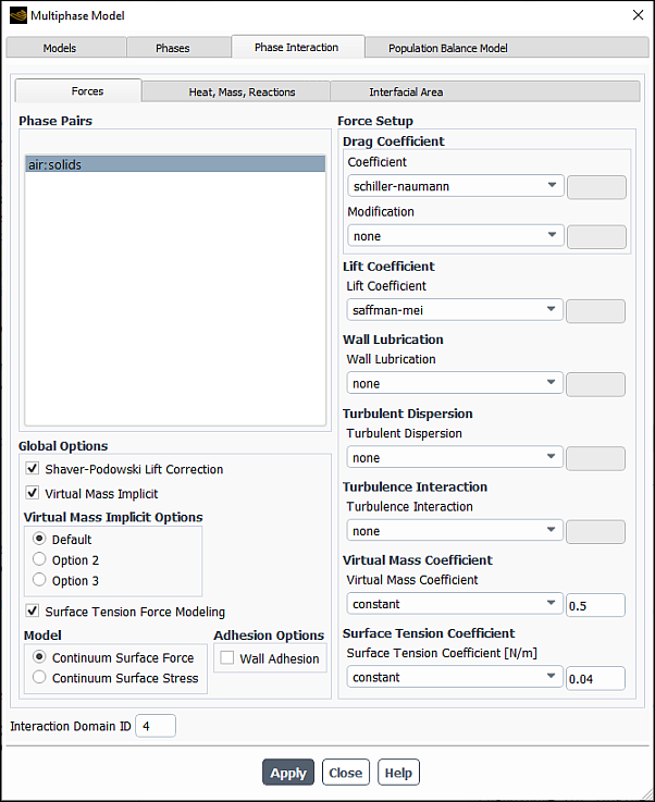
For both granular and non-granular flows, you need to specify the drag function to be used in the calculation of the momentum exchange coefficients. You can also specify lift forces, wall lubrication forces (for non-granular flows only), turbulent dispersion forces, surface tension effects, and virtual mass force. For granular flows, you will also need to specify the restitution coefficient(s) for particle collisions.
To specify these parameters, go to the Phase Interaction > Forces tab in the Multiphase Model dialog box and select appropriate options and values in the Global Options and Force Setup group boxes.
![]() Setup → Models
→ Multiphase
Setup → Models
→ Multiphase
![]() Edit...
Edit...
Ansys Fluent allows you to specify a drag function for each pair of phases.
For each pair of phases, in the Drag coefficient group box, select the one of the following options from the Coefficient drop-down list.
Select ishii to use the fluid-fluid drag function described by Equation 14–516 in the Theory Guide. This option is available when the boiling model is enabled.
Select schiller-naumann to use the fluid-fluid drag function described by Equation 14–215 in the Theory Guide. The Schiller and Naumann model is the default method, and it is acceptable for general use in all fluid-fluid multiphase calculations. When using the homogeneous population balance models you can also select schiller-naumann-pb in which case the interfacial area will be calculated directly from the population balance variables.
Select morsi-alexander to use the fluid-fluid drag function described by Equation 14–219 in the Theory Guide. The Morsi and Alexander model is the most complete, adjusting the function definition frequently over a large range of Reynolds numbers, but calculations with this model may be less stable than with the other models.
Select symmetric to use the fluid-fluid drag function described by Equation 14–225 in the Theory Guide. The symmetric model is recommended for flows in which the secondary (dispersed) phase in one region of the domain becomes the primary (continuous) phase in another. For example, if air is injected into the bottom of a container filled halfway with water, the air is the dispersed phase in the bottom half of the container; in the top half of the container, the air is the continuous phase. The symmetric drag law is the default method for the Multi-Fluid VOF Model, which is available with Eulerian multiphase model.
Select grace to use the fluid-fluid drag function described by Equation 14–230 in the Theory Guide. The Grace model is recommended for gas-liquid flows in which the bubbles can have a range of shapes such as spherical, elliptical, or cap.
In the Grace Swarm Correction dialog box that opens automatically when you first select this model, you can specify Coefficient: Cexp (
 in Equation 14–230 in the Fluent Theory Guide) as constant or
user-defined. Depending on the flow regime and the bubble
size, the following values should be used:
in Equation 14–230 in the Fluent Theory Guide) as constant or
user-defined. Depending on the flow regime and the bubble
size, the following values should be used:Sparsely distributed fluid particles
In flows with sparsely distributed fluid particles,
in Equation 14–230 in the Fluent Theory Guide is zero (default).Densely distributed fluid particles
Since small bubbles tend to rise slowly in high gas volume fractions due to an increase in the effective mixture viscosity, a negative
should be used. The Ishii-Zuber correlation uses an
exponent of -1 for this limit. A value of -0.5 has also been used
successfully by some investigators.Large bubbles, on the other hand, tend to rise faster at high gas volume fractions because they are dragged along by the wakes of other bubbles. This is modeled by using a positive
. The Ishii-Zuber correlation uses an exponent of 2 for
this regime. A value of 4 has also been used successfully by some
researchers in the past
See Grace et al. Model in the Fluent Theory Guide for more information.
Select tomiyama to use the fluid-fluid drag function described by Equation 14–236 in the Theory Guide. Like the Grace model, the Tomiyama model is recommended for gas-liquid flows in which the bubbles can have a range of shapes such as spherical, elliptical, or cap.
Select ishii-zuber to use the fluid-fluid drag function described in Ishii-Zuber Drag Model in the Fluent Theory Guide. The model automatically accounts for swarms of bubbles moving together in high gas volume fractions. Like the Grace and Tomiyama drag models, the Ishii-Zuber drag law is recommended for gas-liquid flows in which bubbles may have a range of shapes such as spherical, elliptical, or cap.
Select anisotropic to use the fluid-fluid drag function described in Multi-Fluid VOF Model in the Theory Guide. The anisotropic drag law is recommended for free surface modeling. It is based on higher drag in the normal direction to the interface and lower drag in the tangential direction to the interface.
Select universal-drag for bubble-liquid and/or droplet-gas flow when the characteristic length of the flow domain is much greater than the averaged size of the droplets/bubbles. It is suitable for flows in which the bubbles/droplets may have a range of shapes. The universal drag law is described using Equation 14–247 in the Theory Guide. When universal-drag is selected, you will need to set a value for the Surface Tension Coefficient. This value will apply to the primary phase and the secondary phase.
Select wen-yu to use the fluid-solid drag function described by Equation 14–282 in the Theory Guide. The Wen and Yu model is applicable for dilute phase flows, in which the total secondary phase volume fraction is significantly lower than that of the primary phase. When using the homogeneous population balance models you can also select wen-yu-pb in which case the interfacial area will be calculated directly from the population balance variables.
Select gidaspow to use the fluid-solid drag function described by Equation 14–284 in the Theory Guide. The Gidaspow model is recommended for dense fluidized beds.
Select syamlal-obrien to use the fluid-solid drag function described by Equation 14–269 in the Theory Guide. The Syamlal-O’Brien model is recommended for use in conjunction with the Syamlal-O’Brien model for granular viscosity.
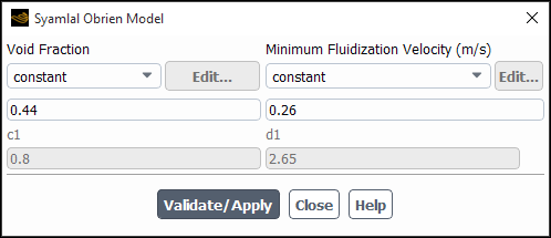
Select syamlal-obrien-para to use the parameterized formulation of the Syamlal-O’Brien model described by Equation 14–279 in the Theory Guide. This model addresses under/over-prediction of bed expansion that can arise with syamlal-obrien. When you first select this model, you will be presented with the Syamlal Obrien Model dialog box.
There are two inputs:
- Void Fraction
the volume fraction of the gas phase in the bed at the minimum fluidization condition
- Minimum Fluidization Velocity
the expected or experimentally-determined nominal minimum fluidization velocity of the gas phase
Once you have input these values, click Validate/Apply to compute the coefficients c1 and d1 used in Equation 14–280 in the Fluent Theory Guide. A message will also be printed to the text user interface summarizing the fluid and flow properties used in the computation and the resulting values. You should check that these property values are consistent with the properties set elsewhere.
Important: If you change property values in the Create/Edit Materials dialog box or diameter for the secondary phase in the Phases tab, you must initialize the flow field or run at least one iteration before computing c1 and d1. Otherwise, incorrect properties will be used in the computation.
Note that the syamlal-obrien-para model is appropriate only for Geldart Group B particles and is only applicable to cases involving a single secondary phase.
Select syamlal-obrien-symmetric to use the solid-solid drag function described by Equation 14–292 in the Theory Guide. The symmetric Syamlal-O’Brien model is appropriate for a pair of solid phases.
Select huilin-gidaspow to use the fluid-solid drag function described by Equation 14–286 in the Theory Guide. This option provides a better blending function for the Gidaspow model when moving from the dense packing limit to the dilute flow limit.
Select gibilaro to use the fluid-solid drag function described by Equation 14–288 in the Theory Guide. This option is used for circulating fluidized beds.
Select emms drag model for gas-solid flow where heterogeneous meso-scale flow structures are dominant and such structures cannot be adequately resolved using fine grid resolution in commercial scale fluidized bed simulation. The fluid-solid drag function is described by Equation 14–290 in the Fluent Theory Guide. The EMMS drag model is applicable only to monodispersed two-phase granular flows without axisymmetric swirl.
Note that this option is not available for non-granular flows.
Select filtered drag model for gas-solid flow cases with coarse meshes. The fluid-solid drag function is computed by Equation 14–290 and Equation 14–488 in the Fluent Theory Guide. Once you click Apply, the following settings are automatically applied to the granular phase properties in the Phases tab:
filtered is selected for Granular Viscosity, Solid Pressure, and Radial Distribution
In the simulation, the radial distribution will be set to zero since the filtered two-fluid model is not based on kinetic theory.
Granular Bulk Viscosity and Granular Temperature are set to a constant value of zero.
For information about how these parameters are calculated, see The Filtered Two-Fluid Model in the Fluent Theory Guide.
In case of convergence issues, you can first run the case with homogeneous drag before switching to the filtered model.
The filtered drag model is applicable only to monodispersed two-phase flows involving gas and granular phases without axisymmetric swirl and is well suited for predicting flow hydrodynamics in fluidized beds.
Select constant to specify a constant value for the drag function, and then specify the value in the text field.
Select user-defined to use a user-defined function for the drag function (see the Fluent Customization Manual for details).
If you want to temporarily ignore the interaction between two phases, select none.
When using the Eulerian or Mixture multiphase models, you can optionally specify a drag modification term for the selected drag law. The drag modification term acts as a multiplier for the drag coefficient computed from the models detailed in Specifying the Drag Function. You can specify the drag modification term individually for each pair of primary-secondary phases. By default, Modification is set to none. To define drag modification, for each pair of phases, select one of the following options from the Modification drop-down list:
constant: Uses a specified constant value for the drag modification factor.
brucato: Uses the Brucato et al. correlation described by Brucato et al. Correlation in the Theory Guide. This modification is appropriate for dilute gas-liquid flows and solid-liquid flows.
wall-drag-enhancement: Uses the wall drag modification described in Near-Wall Drag Enhancement in the Fluent Theory Guide. The modification is useful for improved predictions of the slip velocity in near-wall regions and boiling flow simulations.
user-defined: Uses a user-defined function for the drag modification factor (see
DEFINE_EXCHANGE_PROPERTYin the Fluent Customization Manual for details).
For additional details on the implementation of the drag modification, see Drag Modification in the Theory Guide.
For granular flows, you need to specify the coefficients of
restitution for collisions between particles ( in Equation 14–292 and
  in Equation 14–345 in the Theory Guide). In addition
to specifying the restitution coefficient for collisions between each
pair of granular phases, you will also specify the restitution coefficient
for collisions between particles of the same phase.
in Equation 14–345 in the Theory Guide). In addition
to specifying the restitution coefficient for collisions between each
pair of granular phases, you will also specify the restitution coefficient
for collisions between particles of the same phase.
Perform the following steps:
In the Phases list, select the granular phase pair.
For each pair of granular phases, specify a constant Restitution Coefficient. All restitution coefficients are equal to 0.9 by default.
For both granular and non-granular flows, it is possible to
include the effect of lift forces ( in Equation 14–298 in the Theory Guide) on the secondary phase particles, droplets, or bubbles. These lift
forces act on a particle, droplet, or bubble mainly due to velocity
gradients in the primary-phase flow field. In most cases, the lift
force is insignificant compared to the drag force, so there is no
reason to include it. If the lift force is significant (for example,
if the phases separate quickly), you may want to include this effect.
in Equation 14–298 in the Theory Guide) on the secondary phase particles, droplets, or bubbles. These lift
forces act on a particle, droplet, or bubble mainly due to velocity
gradients in the primary-phase flow field. In most cases, the lift
force is insignificant compared to the drag force, so there is no
reason to include it. If the lift force is significant (for example,
if the phases separate quickly), you may want to include this effect.
Important: Note that the lift force will be more significant for larger particles, but the Ansys Fluent model assumes that the particle diameter is much smaller than the interparticle spacing. Therefore, the inclusion of lift forces is not appropriate for closely packed particles or for very small particles.
To include the effect of lift forces, for each pair of phases, select the appropriate specification method from the Lift Coefficient drop-down list. Note that, since the lift forces for a particle, droplet, or bubble are due mainly to velocity gradients in the primary-phase flow field, you will not specify lift coefficients for pairs consisting of two secondary phases; lift coefficients are specified only for pairs consisting of a secondary phase and the primary phase.
Select none (the default) to ignore the effect of lift forces.
Select constant to specify a constant lift coefficient, and then specify the value in the text field.
Select moraga to use the Moraga lift model (Moraga Lift Force Model in the Theory Guide). The Moraga lift model is applicable to spherical solid particles, drops, and bubbles.
Select saffman-mei to use the Saffman-Mei lift model (Saffman-Mei Lift Force Model in the Theory Guide). The Saffman-Mei lift model is applicable to spherical solid particles, and to drops and bubbles that are not significantly distorted.
Select legendre-magnaudet to use the Legendre—Magnaudet lift model (Legendre-Magnaudet Lift Force Model in the Theory Guide). The Legendre-Magnaudet model is applicable to small diameter spherical fluid particles, though it can be applied to non-distorted liquid drops and bubbles. It accounts for momentum transfer between the flow around the particle and the inner recirculation flow inside the fluid particle caused by fluid friction/stresses at the fluid interface.
Select tomiyama to use the Tomiyama lift model (Tomiyama Lift Force Model in the Theory Guide). The Tomiyama model is applicable to larger-scale deformable bubbles in the ellipsoidal and spherical cap regimes. Its main feature is the prediction of the cross-over point in bubble size at which particle distortion causes a reversal in the sign of the lift force.
Select hessenkemper-et-al to use the Hessenkemper et al. lift model (Hessenkemper et al. Lift Force Model in the Fluent Theory Guide). The Hessenkemper et al. lift model is applicable to small diameter spherical fluid particles and large-scale deformable fluid particles in the ellipsoidal and spherical cap regimes.
Select user-defined to use a user-defined function for the lift coefficient (see the Fluent Customization Manual for details).
When the lift force is included in your simulation, you can enable the Shaver-Podowski Lift Correlation option (Global Options group box). This option improves the accuracy of the prediction of the void peak near the wall and overall robustness when the turbulent dispersion and wall lubrication are used in your case. For more information about this option, see Shaver-Podowski Correction in the Fluent Theory Guide.
For liquid-gas bubbly flows using the Eulerian multiphase model,
you can include the effect of wall lubrication forces ( in Equation 14–194 in the Theory Guide) on the
secondary phase bubbles. These forces tend to push the bubbles away
from walls at small wall distances. For details on how wall lubrication
is modeled in Ansys Fluent see Wall Lubrication Force in the Theory Guide.
in Equation 14–194 in the Theory Guide) on the
secondary phase bubbles. These forces tend to push the bubbles away
from walls at small wall distances. For details on how wall lubrication
is modeled in Ansys Fluent see Wall Lubrication Force in the Theory Guide.
To include the effect of wall lubrication forces, for each pair of phases, select the appropriate specification method from the Wall Lubrication drop-down list. Note that you will specify the wall lubrication only for pairs consisting of a secondary phase and the primary phase.
Select none (the default) to ignore the effect of wall lubrication forces.
Select lubchenko to use the Lubchenko model (Lubchenko Model in the Fluent Theory Guide). This model is available only either burns-et-al or lopez-de-bertodano is selected for the Turbulent Dispersion. If lift is considered in your simulation, you should use the shaver-podowski lift correction.
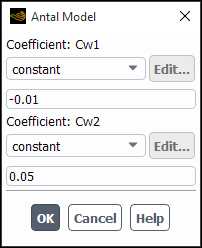
Select antal-et-al to use the Antal et al. model (Antal et al. Model in the Theory Guide). You can edit the model parameters in the Antal Model dialog box (Figure 26.59: Antal et al. Model Dialog Box).
The following model parameters are available:
- Coefficient: Cw1
Specify the constant
 in Equation 14–320 in the Theory Guide. You can enter a constant value or
specify a user-defined function defined using the
in Equation 14–320 in the Theory Guide. You can enter a constant value or
specify a user-defined function defined using the
DEFINE_EXCHANGE_PROPERTYmacro (DEFINE_EXCHANGE_PROPERTY).- Coefficient: Cw2
Specify the constant
 in Equation 14–320 in the Theory Guide. You can enter a constant value or
specify a user-defined function defined using the
in Equation 14–320 in the Theory Guide. You can enter a constant value or
specify a user-defined function defined using the
DEFINE_EXCHANGE_PROPERTYmacro (DEFINE_EXCHANGE_PROPERTY).
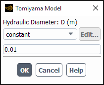
Select tomiyama to use the Tomiyama model (Tomiyama Model in the Theory Guide). This model is only applicable for pipe geometries. You can enter the Hydraulic Diameter for your geometry in the Tomiyama Model dialog box (Figure 26.60: Tomiyama Model Dialog Box).
The following model parameters are available:- Hydraulic Diameter: D (m)
Specify the hydraulic diameter,
 , in Equation 14–322 in the Theory Guide.
Important: The hydraulic diameter must be entered in units of meters.
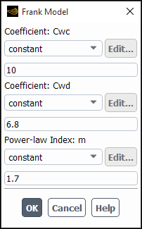
Select frank to use the Frank et al. model (Frank Model in the Theory Guide). You can edit the model parameters in the Frank Model dialog box (Figure 26.61: Frank Model Dialog Box).
The following model parameters are available:
- Coefficient: Cwc
Specify the cutoff coefficient,
 , in Equation 14–324 in the Theory Guide. You can enter a
constant value or specify a user-defined function defined using the
, in Equation 14–324 in the Theory Guide. You can enter a
constant value or specify a user-defined function defined using the
DEFINE_EXCHANGE_PROPERTYmacro (DEFINE_EXCHANGE_PROPERTY).- Coefficient: Cwd
Specify the damping coefficient,
 , in Equation 14–324 in the Theory Guide. You can enter a
constant value or specify a user-defined function defined using the
, in Equation 14–324 in the Theory Guide. You can enter a
constant value or specify a user-defined function defined using the
DEFINE_EXCHANGE_PROPERTYmacro (DEFINE_EXCHANGE_PROPERTY).- Power-law Index: m
Specify the power law constant,
 , in Equation 14–324 in the Theory Guide. You can enter a
constant value or specify a user-defined function defined using the
, in Equation 14–324 in the Theory Guide. You can enter a
constant value or specify a user-defined function defined using the
DEFINE_EXCHANGE_PROPERTYmacro (DEFINE_EXCHANGE_PROPERTY).
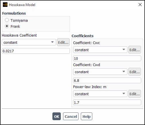
Select hosakawa to use the Hosokawa model (Hosokawa Model in the Theory Guide). You can edit the model parameters in the Hosokawa Model dialog box (Figure 26.62: Hosokawa Model Dialog Box).
The following model parameters are available:
- Formulations
Select which formulation of the Hosokawa model to use. You can select either Frank or Tomiyama.
- Hosokawa Coefficient
Specify the coefficient of the Eotvos number in Equation 14–325 in the Theory Guide. You can enter a constant value or specify a user-defined function defined using the
DEFINE_EXCHANGE_PROPERTYmacro (DEFINE_EXCHANGE_PROPERTY).- Coefficients
Specify the model parameters associated with the formulation you selected under Formulations.
Select user-defined to use a user-defined function for the wall lubrication coefficient (see
DEFINE_EXCHANGE_PROPERTYin the Fluent Customization Manual for details).
For turbulent flows using the Eulerian multiphase model, you
can include the effects of turbulent dispersion force ( in Equation 14–194 in the Theory Guide). The turbulent
dispersion force acts as a turbulent diffusion in dispersed flows.
For details on how turbulent dispersion is modeled in Ansys Fluent see Turbulent Dispersion Force in the Theory Guide.
in Equation 14–194 in the Theory Guide). The turbulent
dispersion force acts as a turbulent diffusion in dispersed flows.
For details on how turbulent dispersion is modeled in Ansys Fluent see Turbulent Dispersion Force in the Theory Guide.
To include the effects of turbulent dispersion force, for each pair of phases, select the appropriate specification method from the Turbulent Dispersion drop-down list. Note that you will specify the turbulent dispersion only for pairs consisting of a secondary phase and the primary phase.
Select none (the default) to ignore the effects of turbulent dispersion.
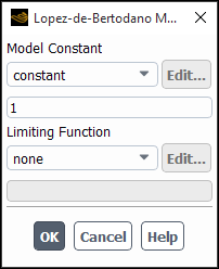
Select lopez-de-bertodano to use the Lopez de Bertodano model (Lopez de Bertodano Model in the Theory Guide). You can edit the model parameters in the Lopez de Bertodano Model dialog box (Figure 26.63: Lopez de Bertodano Model Dialog Box).
The following model parameters are available:
- Model Constant
Specify the coefficient,
 , in Equation 14–332 in the Theory Guide. You can enter a
constant value or specify a user-defined function defined using the
, in Equation 14–332 in the Theory Guide. You can enter a
constant value or specify a user-defined function defined using the
DEFINE_EXCHANGE_PROPERTYmacro (DEFINE_EXCHANGE_PROPERTY).- Limiting Function
Specify the limiting function to use. You may select none, the standard limiting function, or a user-defined function using the
DEFINE_EXCHANGE_PROPERTYmacro (DEFINE_EXCHANGE_PROPERTY). See Limiting Functions for the Turbulent Dispersion Force in Fluent Theory Guide for details on the limiting functions.
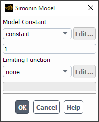
Select simonin to use the Simonin model (Simonin Model in the Theory Guide).
You can specify the model parameters in the Simonin Model dialog box (Figure 26.64: Simonin Model Dialog Box).
The following model parameters are available:
- Model Constant
Specify the coefficient,
 , in Equation 14–334 in the Theory Guide. You can enter a
constant value or specify a user-defined function defined using the
, in Equation 14–334 in the Theory Guide. You can enter a
constant value or specify a user-defined function defined using the
DEFINE_EXCHANGE_PROPERTYmacro (DEFINE_EXCHANGE_PROPERTY).- Limiting Function
Specify the limiting function to use. You may select none, the standard limiting function, or a user-defined function using the DEFINE_EXCHANGE_PROPERTY macro (
DEFINE_EXCHANGE_PROPERTY). See Limiting Functions for the Turbulent Dispersion Force in Fluent Theory Guide for details on the limiting functions.
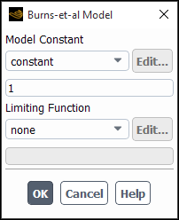
Select burns-et-al to use the Burns et al. model (Burns et al. Model in the Theory Guide). You can edit the model parameters in the Burns-et-al Model dialog box (Figure 26.65: Burns et al. Model Dialog Box).
The following model parameters are available:
- Model Constant
Specify the coefficient,
 , in Equation 14–337 in the Theory Guide. You can enter a
constant value or specify a user-defined function defined using the
, in Equation 14–337 in the Theory Guide. You can enter a
constant value or specify a user-defined function defined using the
DEFINE_EXCHANGE_PROPERTYmacro (DEFINE_EXCHANGE_PROPERTY).- Limiting Function
Specify the limiting function to use. You may select none, the standard limiting function, or a user-defined function using the
DEFINE_EXCHANGE_PROPERTYmacro (DEFINE_EXCHANGE_PROPERTY). See Limiting Functions for the Turbulent Dispersion Force in Fluent Theory Guide for details on the limiting functions.
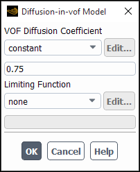
Select diffusion-in-vof to use the Diffusion in VOF model (Diffusion in VOF Model in the Theory Guide). You can edit the model parameters in the Diffusion-in-vof Model dialog box (Figure 26.66: Diffusion—in—vof Model Dialog Box).
The following model parameters are available:
- VOF Diffusion Coefficient
Specify the coefficient,
 , in Equation 14–340 in the Theory Guide.
- Limiting Function
Specify the limiting function to use. You may select none, the standard limiting function, or a user-defined function using the
DEFINE_EXCHANGE_PROPERTYmacro (DEFINE_EXCHANGE_PROPERTY). See Limiting Functions for the Turbulent Dispersion Force in Fluent Theory Guide for details on the limiting functions.
Select user-defined to use a user-defined function for the turbulent dispersion (see
DEFINE_VECTOR_EXCHANGE_PROPERTYin the Fluent Customization Manual for details).
As discussed in When Surface Tension Effects Are Important in the Theory Guide, the importance of surface
tension effects depends on the value of the capillary number, Ca (defined by Equation 14–32 in the Theory Guide), or the Weber number, We
(defined by Equation 14–33 in the Theory Guide). Surface tension effects
can be neglected if Ca  or We
or We  .
.
Important: Note that the calculation of surface tension effects will be more accurate if you use a quadrilateral or hexahedral mesh in the area(s) of the computational domain where surface tension is significant. If you cannot use a quadrilateral or hexahedral mesh for the entire domain, then you should use a hybrid mesh, with quadrilaterals or hexahedra in the affected areas. Ansys Fluent also offers an option to use VOF gradients at the nodes for curvature calculations on meshes when more accuracy is desired. For more information, see Surface Tension and Adhesion in the Theory Guide.
If you want to include the effects of surface tension along the interface between one or more pairs of phases, as described in Surface Tension and Adhesion in the Theory Guide, refer to Including Surface Tension and Adhesion Effects.
For both granular and non-granular flows, it is possible to
include the “virtual mass force” ( in Equation 14–343 in the Theory Guide) that is
present when a secondary phase accelerates relative to the primary
phase. The virtual mass effect is significant when the secondary phase
density is much smaller than the primary phase density (for example,
for a transient bubble column).
in Equation 14–343 in the Theory Guide) that is
present when a secondary phase accelerates relative to the primary
phase. The virtual mass effect is significant when the secondary phase
density is much smaller than the primary phase density (for example,
for a transient bubble column).
To include the effect of the virtual mass force perform the following steps:
For each phase pair, select the method for specifying the Virtual Mass Coefficient,
 , in Equation 14–343 in the Fluent Theory Guide. You can choose from the following methods:
- none
Disable virtual mass modeling for the phase pair.
- constant
Specify a constant value for the coefficient. The default value of
0.5is typical.- user-defined
Use a user-defined function created with the
DEFINE_EXCHANGE_PROPERTYmacro. SeeDEFINE_EXCHANGE_PROPERTYin the Fluent Customization Manual for details.
If desired, you can enable the Virtual Mass Implicit method.
When using the Virtual Mass Implicit method, the Default option uses the complete term in Equation 14–343. You can also choose Option 2 or Option 3, which use locally truncated forms of the virtual mass terms in cells where divergence is detected.
The Virtual Mass Implicit method is recommended for steady-state coupled simulations as it offers improved convergence in such cases. The recommended approach is to begin the simulation using Option 2. Once the solution has converged enough to establish the basic flow field, switch back to Default to include the complete virtual mass term.
If you are using the Eulerian model to solve a turbulent flow, you will need to choose one of turbulence models described in Turbulence Models in the Theory Guide in the Viscous Model Dialog Box (Figure 26.67: The Viscous Model Dialog Box for an Eulerian Multiphase Calculation).
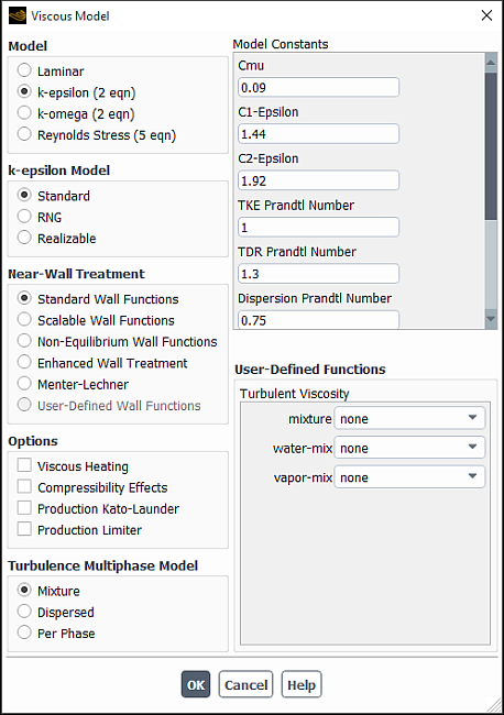
The procedure is as follows:
Select k-epsilon, k-omega, or Reynolds Stress under Model.
Select the desired k-epsilon Model, k-omega Model, or Reynolds-Stress Model and any other related parameters, as described for single-phase calculations in Steps in Using a Turbulence Model.
Under Turbulence Multiphase Model or RSM Multiphase Model, indicate the desired multiphase turbulence model (see Turbulence Models in the Theory Guide for details about each):
Select Mixture to use the mixture turbulence model. This is the default model.
Select Dispersed to use the dispersed turbulence model. This model is applicable when there is clearly one primary continuous phase and the rest are dispersed dilute secondary phases.
Select Per Phase to use a
 -
-  or
or  -
-  turbulence model
for each phase. This model is appropriate when the turbulence transfer
among the phases plays a dominant role.
turbulence model
for each phase. This model is appropriate when the turbulence transfer
among the phases plays a dominant role.
By default, interphase turbulence source terms are not included in the calculation. If you want to include these source terms, you can define them in the Forces tab of the Multiphase Model Dialog Box.
![]() Setup → Models
→ Multiphase
Setup → Models
→ Multiphase
![]() Edit...
Edit...
For each pair of phases, select the desired correlation for the Turbulence Interaction (Forces Setup group box):
select none to omit turbulence interaction source terms. This is the default.
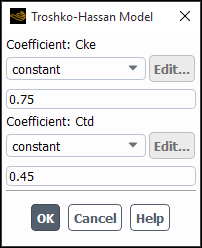
select troshko-hassan to use the Troshko-Hassan model described in Troshko-Hassan in the Fluent Theory Guide. You can edit the model parameters in the Troshko-Hassan Model dialog box (Figure 26.68: Troshko-Hassan Model Dialog Box).
The following model parameters are available:
- Coefficient: Cke
Specify the coefficient,
 , in the equations in Troshko-Hassan in the Fluent Theory Guide.
- Coefficient: Ctd
Specify the coefficient,
 , in the equations in Troshko-Hassan in the Fluent Theory Guide.
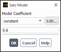
select sato to use the Sato model described in Sato in the Fluent Theory Guide. You can edit the model parameters in the Sato Model dialog box (Figure 26.69: Sato Model Dialog Box).
The following model parameters are available:
- Model Coefficient
Specify the coefficient,
 , in the equations in Sato in the Fluent Theory Guide.
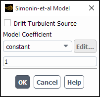
select simonin-et-al to use the Simonin et al. model described in Simonin et al. in the Fluent Theory Guide. This option is available only when Dispersed or Per Phase is selected in the Viscous Model dialog box. You can edit the model parameters in the Simonin-et-al Model dialog box (Figure 26.70: Simonin-et-al Model Dialog Box).
The following model parameters are available:
- Drift Turbulent Source
include the portion the turbulent kinetic energy source term arising from the drift velocity.
- Model Coefficient
Specify the coefficient,
 , in the equations in Simonin et al. in the Fluent Theory Guide.
If you decide to enable turbulence interaction for multiple phase pairs, it is recommended that you avoid mixing the different models and that you select the same model for each phase pair with turbulence interaction enabled.
Note that the inclusion of these terms can slow down convergence noticeably. If you are looking for additional accuracy, you may want to compute a solution first without these sources, and then continue the calculation with these terms included. In most cases these terms can be neglected.
If you are using the  -
-  multiphase turbulence model, a user-defined
function can be used to customize the turbulent viscosity for each
phase. This option will enable you to modify
multiphase turbulence model, a user-defined
function can be used to customize the turbulent viscosity for each
phase. This option will enable you to modify  in the
  -
-  model. For more information,
see the Fluent Customization Manual.
model. For more information,
see the Fluent Customization Manual.
In the Viscous Model dialog box, under User-Defined Functions, select the appropriate user-defined function in the Turbulent Viscosity drop-down list.
To define heat transfer in a multiphase Eulerian simulation, after you have enabled the energy equation in the Energy dialog box, you need to visit the Phase Interaction > Heat, Mass, Reactions > Heat tab in the Multiphase Model dialog box.
![]() Setup → Models →
Multiphase
Setup → Models →
Multiphase ![]() Edit...
Edit...
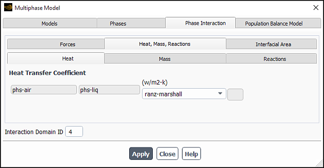
Select the desired correlation for the Heat Transfer Coefficient. See The Heat Exchange Coefficient in the Fluent Theory Guide for more information. The available choices are as follows and depend on what other models you have enabled:
- constant-htc
allows you to specify a constant value for the volumetric heat transfer coefficient. See Constant in the Fluent Theory Guide for details.
- nusselt-number
allows you to specify a value for the Nusselt number from which the heat transfer coefficient will be computed. See Nusselt Number in the Fluent Theory Guide for details.
- gunn
is frequently used for Eulerian multiphase simulations involving a granular phase. See Gunn Model in the Fluent Theory Guide for details.
- ranz-marshall
is frequently used for Eulerian multiphase simulations not involving a granular phase. See Ranz-Marshall Model in the Fluent Theory Guide for details.
- hughmark
is an extension of Ranz-Marshall to a wider range of Reynolds Number. See Hughmark Model in the Fluent Theory Guide for details.
- tomiyama
is frequently used for Eulerian multiphase simulations of bubbly flows with relatively low Reynolds number. See Tomiyama Model in the Fluent Theory Guide for details.
- none
allows you to ignore the effects of heat transfer between the two phases.
- user-defined
allows you to implement a correlation reflecting a model of your choice, through a user-defined function.
- fixed-to-sat-temp
models heat transfer when all of the heat transfer to a phase interface is used in mass transfer. It assumes that the temperature at the To-Phase in the mass transfer is equal to the saturation temperature. Note that this model is available only when Boiling is disabled in the Models tab of the Multiphase Model dialog box.
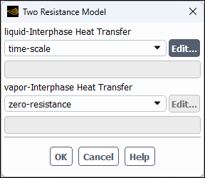
- two-resistance
opens the Two Resistance Model dialog box where you can independently specify the heat transfer coefficient correlations for the two phases.
In addition to heat transfer coefficient models described above, the following sub-models of the two-resistance model are available:
- time-scale
models the gas-interface heat transfer coefficient. It assumes that the gas phase retains the saturation temperature by rapid evaporation or condensation.
- zero-resistance
when selected for one of the phases, the phase temperature will be equal to the interfacial temperature. Note that you should not select this option for both interphase heat transfer coefficients.
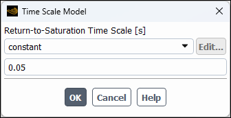
When time-scale is selected, the Time Scale Model dialog box opens automatically where you need to specify a positive non-zero value for the Return-to-Saturation Time Scale (
 in Equation 14–396 in the Fluent Theory Guide).
This option is recommended when using the evaporation-condensation mass transfer model. See Two-Resistance Model in the Fluent Theory Guide for details.
Note: When using multiple boiling mechanisms (such as in boiling coupled with the inhomogeneous PBM), the two-resistance heat transfer option is not recommended for phase pairs with the boiling mass transfer option as it may result in incorrect solution. Instead, use the two-resistance boiling framework that is enabled via the Text User Interface (TUI) as described in Including the Boiling Model.
Set the appropriate thermal boundary conditions. You will specify the thermal boundary conditions for each individual phase on most boundaries, and for the mixture on some boundaries. See Cell Zone and Boundary Conditions for more information on boundary conditions, and Eulerian Model for more information on specifying boundary conditions for a Eulerian multiphase calculation.
See Description of Heat Transfer in the Theory Guide for more information on heat transfer in the framework of a Eulerian multiphase simulation and the available models.
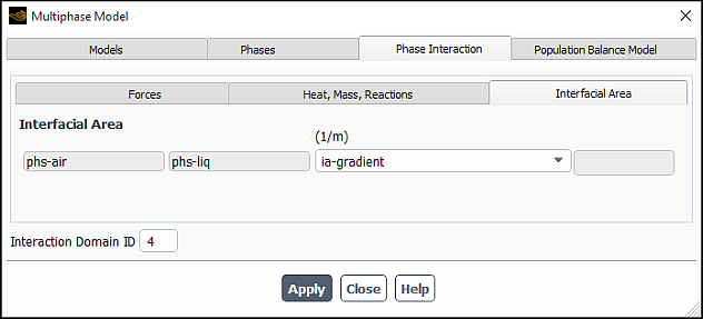
If you have chosen not to solve the transport equation for Interfacial Area Concentration (Defining the Interfacial Area Concentration), you can select an algebraic model to estimate the interfacial area from the secondary phase diameter specified in the Interfacial Area tab of the Multiphase Model dialog box. To choose an algebraic interfacial area model perform these steps.
In the Multiphase Model dialog box, go to the Phase Interaction > Interfacial Area tab box (for example, Figure 26.74: The Multiphase Model Dialog Box for Interfacial Area).
In the Interfacial Area tab, select the desired algebraic model for the Interfacial Area. Note the following regarding the available choices:
- ia-symmetric
considers both the primary and secondary phase volume fractions in estimating the interfacial area.
- ia-particle
considers only the secondary phase volume fraction in estimating the interfacial area.
- ia-gradient
considers the volume fraction gradient at the interface between two phases in estimating the interfacial area.
Additional options are available if you have enabled one of the boiling models. See Including the Boiling Model.
See Interfacial Area Concentration in the Fluent Theory Guide for details about the algebraic interfacial area models.
The Algebraic Interfacial Area Density (AIAD) model is available only within the Eulerian multiphase framework and cannot be used with the following models:
Dense Discrete Phase Model (DDPM)
Boiling model
To use the Algebraic Interfacial Area Density (AIAD) model, follow the steps outlined below. Only the steps that are pertinent to the AIAD modeling are listed here. For the theory behind the AIAD model, see Algebraic Interfacial Area Density (AIAD) Model in the Fluent Theory Guide.
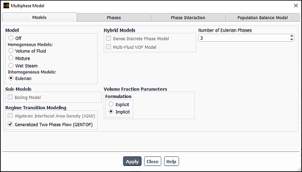
In the Multiphase Model dialog box, select Eulerian (in the Model group box) and Algebraic Interfacial Area Density (AIAD) (in the Regime Transition Modeling group box).
 Setup → Models
→ Multiphase
Setup → Models
→ Multiphase Edit...
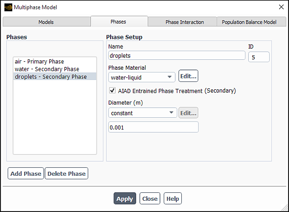
Important: Only two Eulerian phases are required for the AIAD model. However, if you want to model phase entrainment, then at least one additional secondary phase must be defined in your simulation.
Phase entrainment and absorption are modeled through the aiad-entrained-absorption mass transfer mechanism as further described. For example, if you want to model droplet entrainment, define gas as a primary phase, liquid as a secondary continuous phase, and droplets as a secondary entrained phase. Bubble entrainment can be modeled in a similar manner. In bubble entrainment modeling, define liquid as a primary continuous phase, gas as a secondary continuous phase, and bubbles as a secondary entrained phase. The AIAD model implementation requires both secondary phases to be of the same material.
Click Apply.
Important: When setting up your case, if you have made changes in the current tab, you should click the button to make them effective before moving to the next tab. Otherwise, the relevant models may not be available in the other tabs, and your settings may be lost.
Once the AIAD model is applied, Ansys Fluent automatically selects the following options in the Multiphase Model dialog box:
Multi-Fluid VOF Model (Hybrid Models group box)
Sharp/Dispersed interface modeling type (Options group box)
Phase Localized Discretization (Interface Modeling Options dialog box)
Note: Although these options are displayed in the Models tab, they cannot be accessed when the Algebraic Interfacial Area Density (AIAD) is selected.
In the Phases tab, set the phases for your simulation.
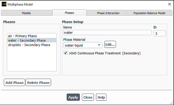
Define the primary and secondary phases as appropriate. Note that AIAD Continuous Phase Treatment (Primary) is automatically selected for the primary phase.
For one of the secondary phases, assign a different phase material than that of the primary phase and then select the AIAD Continuous Phase Treatment (Secondary) option.
If you are modeling phase entrainment, then define the other secondary phase as follows:
Click Apply.
In the Phase Interaction tab, define the interaction between the phases.
In the Forces tab, set the interfacial forces between the phase pairs.
Note the following when using the AIAD model:
For the pair of the primary and AIAD secondary continuous phases, you can define only the drag and surface tension coefficients.
The pair of the primary and secondary entrained phases has no restrictions in terms of setting interfacial forces.
The two phases of the same material (AIAD continuous and entrained) interact via entrainment and deposition. No forces should be defined for such phase pairs.
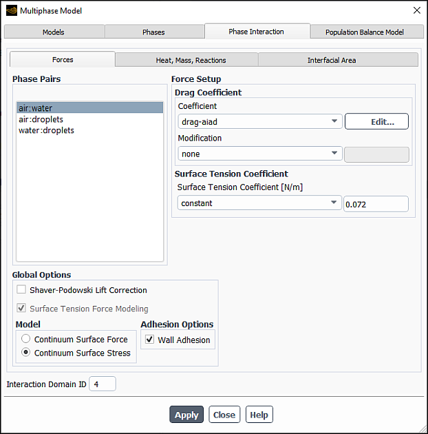
Once the Algebraic Interfacial Area Density (AIAD) model is applied, Ansys Fluent automatically selects the following options:
Surface Tension Force Modeling and Continuum Surface Stress (Global Options group box)
Although the Surface Tension Force Modeling option cannot be overridden, you can select a surface tension and adhesion methods suitable for your simulation.
drag-aiad for the drag Coefficient for the pair of the primary and AIAD secondary continuous phases
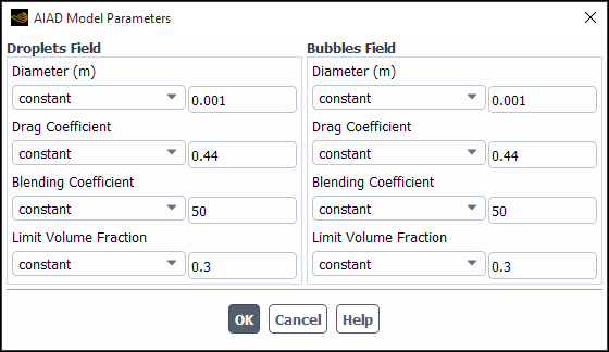
You can click Edit... next to the Coefficient text entry field and adjust values of the AIAD model parameters in the AIAD Model Parameters dialog box.
You can specify the following parameters in the Droplets Field and Bubbles Field group boxes:
Diameter:
 and
and  in Equation 14–458 and Equation 14–459 in the Fluent Theory Guide
Drag Coefficient:
 and
and  in Equation 14–470 in the Fluent Theory Guide
You can specify the drag coefficients for both droplet and bubbles files using either constant values or the user-defined option and use the DEFINE_EXCHANGE_PROPERTY user-defined function to define these inputs. See section "DEFINE_EXCHANGE_PROPERTY" in the Fluent Customization Manual for details.
Blending Coefficient:
 and
and  in Equation 14–455 in the Fluent Theory Guide and Equation 14–456 in the Fluent Theory Guide, respectively
Limit Volume Fraction:
 and
and  in Equation 14–455 in the Fluent Theory Guide and Equation 14–456 in the Fluent Theory Guide, respectively
The default values for Drag Coefficient, Blending Coefficient, and Limit Volume Fraction are suitable for most cases that involve the AIAD model.
If you are modeling phase entrainment, then in the Heat, Mass, Reactions tab, Ansys Fluent automatically selects the aiad-entrained-absorption mechanism for mass transfer from the AIAD secondary continuous phase to the entrained secondary phase. The mass transfer rate is positive when the entrainment mechanism is dominant and negative when the absorption mechanism is dominant.
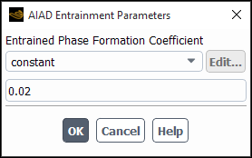
If you want to adjust a value for
 in Equation 14–478 in the Fluent Theory Guide), click Edit... next to the selected mechanism and enter a new
value in the Entrained Phase Formation Coefficient text entry
field in the AIAD Entrainment Parameters dialog box.
in Equation 14–478 in the Fluent Theory Guide), click Edit... next to the selected mechanism and enter a new
value in the Entrained Phase Formation Coefficient text entry
field in the AIAD Entrainment Parameters dialog box.For more information about the aiad-entrained-absorption mass transfer mechanism, see Modeling Entrainment-Absorption in the Fluent Theory Guide.
Note: The aiad-entrained-absorption mechanism cannot be removed unless the AIAD Entrained Phase Treatment (Secondary) option is cleared for the relevant phase in the Phases tab.
In the Interfacial Area tab, select the interfacial area method for phase pairs.
Ansys Fluent automatically assigns the ia-aiad interfacial area algebraic model for the AIAD phase pair. This is the only model available for the AIAD phase pair. There are no restrictions for the other phase pairs.
If you are using the entrained phase in your simulation, you can set up the population balance model in the Population Balance Model tab to predict the growth of the droplet phase and entrained particle distribution. You can use the aggregation and breakage kernels from and to the entrained phase.
For information on how to set up the population balance simulation, see Population Balance Model .
In the Viscous Model dialog box, the ANSYS Fluent solver has automatically enables the following models and options:
k-omega SST turbulence model
Turbulence Damping (Turbulence Damping Options group box)
This option affects only the continuous phases (primary and AIAD secondary continuous phases)
Per Phase (Options group box)
Subrgid Turbulence Contribution (AIAD) (Regime Transition Modeling group box)
This option adds an extra source to the turbulent kinetic energy. For more information, see Modeling Sub-grid Wave Turbulence Contribution (SWT) in the Fluent Theory Guide.
These models and options are best suitable for simulations that involve the AIAD model; however, you can override these settings (except for the Per Phase option) for your current simulation.
Ansys Fluent automatically enables gravity for the AIAD model. Make sure that the gravitational field is correctly specified in the General task page.
Due to the nature of the problems that involve the AIAD model, the Transient solver has been automatically selected for the AIAD model. However, you can use the steady-state solver for your current AIAD case. Selecting Global Time Step from the Pseudo Time Method list (in the Solution Methods task page) is recommended for such cases, which is available with the Coupled scheme for the pressure-velocity coupling.
In the Solution Controls task page, the Under-Relaxation Factors have been changed to more conservative values as recommended for the AIAD model. Depending on your problem and the convergence behavior of your simulation, you can adjust these values to better suit your specific case.
If a convergence problem arises when solving a case that involves the phase entrainment model, you can try running the simulation without entrainment, and then continuing running with the AIAD Entrained Phase Treatment (Secondary) option, which automatically adds the aiad-entrainment-absorption mass transfer mechanism. You can also lower the Vaporization Mass relaxation factor (default: 1.0). This can be reduced to as low as 0.2, depending of the complexity of the problem.
To improve accuracy, you can increase the under-relaxation factors for your AIAD simulation depending on the convergence behavior of the calculation.
The GENTOP model is available only within the Eulerian multiphase framework and cannot be used with the following models:
Multi-fluid VOF model
Dense discrete phase model (DDPM)
Boiling model
Species transport model
The procedure for setting up a flow regime transition simulation using the GENTOP model is described below. Note that only steps that are pertinent to the GENTOP model are shown. For theoretical information about the GENTOP model, see Generalized Two Phase (GENTOP) Flow Model in the Fluent Theory Guide.
In the Multiphase Model dialog box, select the Eulerian inhomogeneous model and Generalized Two Phase Flow (GENTOP) (Regime Transition Modeling group box).
Setup →
Models →
Multiphase
Edit...
Ansys Fluent automatically makes the following changes:
Adds three Eulerian phases
You can include more than two secondary phases in your simulation.
In the Heat, Mass, Reactions tab, automatically selects the gentop-complete-coalescence mechanism for transferring mass from secondary non-GENTOP phases to the GENTOP phase.
Applies the following settings to the population balance model:
Enables the Inhomogeneous Discrete method
Defines Bins for all relevant active secondary phases. For the GENTOP phase, only one bin with the largest diameter size is assigned.
Enables the Aggregation and Breakage kernels to allow the growth to occur between the active secondary phases and the GENTOP phase.
Note that these settings cannot be modified.
Specify the Calibration Coefficient (
 in Equation 14–483 in the Fluent Theory Guide). The default value of 1.0 is acceptable for most regime transition / mixing
problems.
in Equation 14–483 in the Fluent Theory Guide). The default value of 1.0 is acceptable for most regime transition / mixing
problems.Click Apply.
In the Phases tab, define the phases for your simulation.
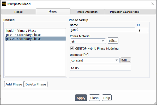
Note the following:
For one of the secondary phases, you must select GENTOP Hybrid Phase Modeling.
All the secondary phases must share the same material, which must be different than that of the primary phase.
Click Apply.
In the Phase Interaction tab, define the interaction between the phases.
In the Forces tab, set the interfacial forces between the phase pairs.
When setting the primary-GENTOP phase pair, note the following:
Only ishii-zuber, grace, and universal-drag are available for the Drag Coefficient specification.
There is no limitations on using lift, wall lubrication, and virtual mass models as well as all options for the surface tension coefficient that are available in Ansys Fluent.
Turbulent dispersion and turbulence interaction models are not available.
For other phase pairs, no limitation exists on using the Ansys Fluent force interaction models.
Click Apply.
In the Population Balance Model tab, check and modify the available settings as needed (such as the number of bins, breakage and aggregation kernels and submodels, and so on).
Click Apply.
Proceed with the simulation as usual.
If any convergence issues arise, you can try to lower the relaxation factors and follow the solution strategies for improving convergence for Eulerian flows outlined in Eulerian Model.
You can also try using the Coupled solver to improve solver robustness.
To improve accuracy, you can decrease the default under-relaxation factors, depending on the convergence behavior of the calculation.
If you are using the Eulerian multiphase model (Setting Up the Eulerian Model), you have the option of including the dense discrete phase mode (DDPM) (Dense Discrete Phase Model in the Theory Guide).
Important:
Enabling this model automatically enables the DPM model. You will notice that Interaction with Continuous Phase in the Discrete Phase Model dialog box is enabled.
The dense discrete phase model is available only with the Eulerian multiphase model. The limitations that currently apply to DPM and Eulerian multiphase models also apply to the dense discrete phase model. See Limitations of the Eulerian Model in the Fluent Theory Guide and Limitations for limitations that exist with the DPM and Eulerian multiphase models.
The required work flow when using the dense discrete phase model is as follows:
In the Multiphase Model dialog box, enable the DDPM (Models tab) (Figure 26.79: The Dense Discrete Phase Model - Models Tab).
Setup →  Models →
  Multiphase → Edit...
Select Dense Discrete Phase Model in the Hybrid Models group box.
Specify the Number of Discrete Phases that are present in your case.
Click .
Once the DDPM is enabled, Ansys Fluent automatically applies the following changes in the Multiphase Model dialog box:
averaged-discrete-phase-drag is selected for the Drag Coefficient (Phase Interaction > Forces tab).
averaged-discrete-phase-drag corresponds to
 in Equation 14–498 in the Fluent Theory Guide and indicates that the interaction between discrete
and fluid phases will be computed based on averaged values of fluid drag of all
particles crossing the fluid cell. That is, at each time step, the drag is evaluated
for each particle using the drag law that you have selected in the Set
injection Properties dialog box and then averaged based on the
residence time of each particle in the cell.
in Equation 14–498 in the Fluent Theory Guide and indicates that the interaction between discrete
and fluid phases will be computed based on averaged values of fluid drag of all
particles crossing the fluid cell. That is, at each time step, the drag is evaluated
for each particle using the drag law that you have selected in the Set
injection Properties dialog box and then averaged based on the
residence time of each particle in the cell.(cases with energy transfer) averaged-discrete-phase-heat is selected for the Heat Transfer Coefficient (Phase Interaction > Heat, Mass, Reactions > Heat tab).
averaged-discrete-phase-heat corresponds to the heat exchange coefficient
 in Equation 14–500 in the Fluent Theory Guide and indicates that the interaction between the
discrete and fluid phases will be computed based on the averaged heat transfer
between the fluid and all particles crossing the fluid cell. The heat transfer law
that is used to evaluate the heat exchange is the law that you have selected in the
Set injection Properties dialog box. The contribution of each
particle to the averaged heat transfer is based on the residence time of the
particle in the cell.
in Equation 14–500 in the Fluent Theory Guide and indicates that the interaction between the
discrete and fluid phases will be computed based on the averaged heat transfer
between the fluid and all particles crossing the fluid cell. The heat transfer law
that is used to evaluate the heat exchange is the law that you have selected in the
Set injection Properties dialog box. The contribution of each
particle to the averaged heat transfer is based on the residence time of the
particle in the cell.
In the Phases tab, define the phases.
Define the discrete phase, by selecting the phase from the Phases selection list that is labeled Discrete Phase. Then set up the properties in the Phase Setup group box (for example, Figure 26.80: The Multiphase Model Dialog Box for DDPM).
Note that for non-granular flow, no additional inputs are required here (since the material is set automatically in the background, and the diameter is part of the solution).
To prevent particle concentration from becoming unphysically high, enable Volume Fraction Approaching Continuous Flow Limit and specify Transition Factor. The criterion of transition from the standard method to a special treatment is specified as multiplied by the theoretical close-packing limit for mono-sized spheres (
 ). If the particle volume fraction exceeds this transition volume fraction, Ansys Fluent will apply a special treatment to the particle momentum equation. For more information, refer to Dense Discrete Phase Model in the Fluent Theory Guide.
The default value for the Transition Factor is 0.75, giving a transition volume fraction of 0.5625 (=0.75*3/4). Note that the Transition Factor is not limited to a range between 0 and 1. In other words, you can specify values outside this range. For example, a value of 1.2 will give a transition volume fraction of 0.9. You can also specify locally variable values using the
DEFINE_PROPERTYuser-defined macro, depending on the local particle size distribution, as an example.See
DEFINE_PROPERTYUDFs in the Fluent Customization Manual for information about theDEFINE_PROPERTY.Define the primary and secondary phases, as described in Defining the Phases for the Eulerian Model.
Define the injections using the Injections dialog box.
Setup → Models → Discrete Phase → Injections New...
Create a new injection by clicking the button in the Injections dialog box, or edit an existing injection by selecting the injection from the Injections list and clicking the button.
In the Set Injection Properties dialog box that opens (Figure 26.81: The Set Injection Properties Dialog Box), specify properties for each injection as described in Setting Initial Conditions for the Discrete Phase
Select the discrete phase from the Discrete Phase Domain drop-down list.
(cases with the energy equation enabled) By default, Ansys Fluent uses the heat exchange coupling formulation described in Equation 14–499 in the Fluent Theory Guide to model the energy interaction with the primary phase. One part of the energy transfer is provided via
 , and the rest is included in the source term
  .
. For simulations with poly-dispersed particles that use the default heat exchange coupling, it is recommended that you enable the enhanced Eulerian interphase exchange using the following text command:
define/models/dpm/interaction/ddpm-enhanced-inter-phase-exchange?Apply enhanced inter-phase exchange? [no]yesAs an alternative to the default coupling formulation, you can use the following text command options for the energy interaction with the primary phase:
Energy coupling purely via the source terms:
define/models/dpm/interaction/ddpm-energy-coupling-via-source-term?Establish energy coupling in DDPM via source term? [no]yesWith this option enabled, the interaction is achieved purely through an explicit source term
in Equation 14–499 in the Fluent Theory Guide. The heat exchange term is not used for this coupling. This option can accelerate the
solution for flows with either low to moderate particle load or small particles. Energy coupling via the linearized source terms:
define/models/dpm/interaction/linearized-dpm-source-terms?Linearize the DPM source terms? [no]yesThis option may help stabilize the solution in cases where it is unstable due to the high particle volume fraction and/or the high particle-to-fluid density ratio. This coupling can be used only when the energy coupling via the source terms is enabled. Otherwise, the default coupling formulation will be used for all injections with the Discrete Phase Domain set to anything other than none, and the source term linearization will be applied only to non-DDPM injections.
Define the material properties for each injection.
Setup → Materials
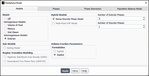
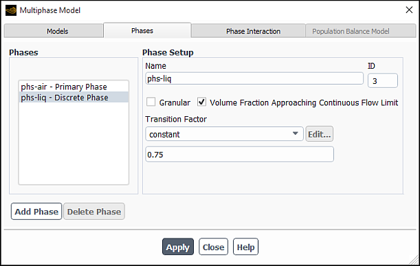
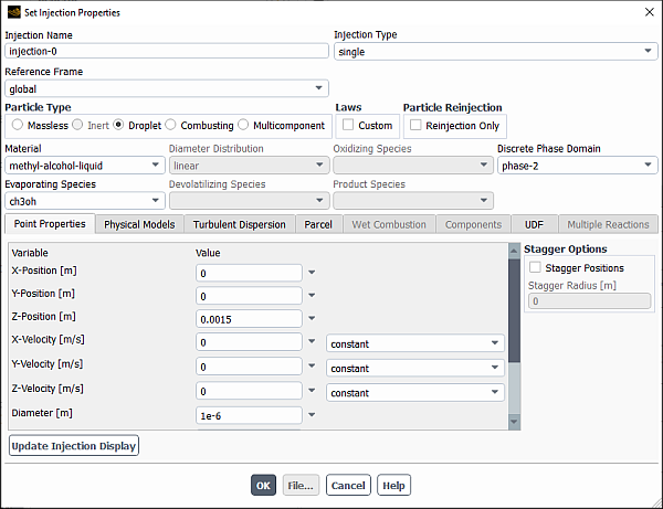
To define a granular (that is, particulate) discrete phase in an Eulerian multiphase calculation, perform the following steps:
Select the phase (for example, Figure 26.82: The Multiphase Model Dialog Box for a Granular Phase) in the Phases list. Then set up the properties in the Phase Setup group box (for example, (Figure 26.82: The Multiphase Model Dialog Box for a Granular Phase)
Enter a Name for the phase.
Enable the Granular option.
Enable Volume Fraction Approaching Packing Limit to prevent the unlimited accumulation of particles, which are operating at packing limit conditions.
Note: To reduce excessive accumulation of particles in cells, you can also enable the Enhanced Numerics option in the Discrete Phase Model dialog box (Numerics tab). Enhanced numerics is applied to particles of granular phases only. This option can be used with or without the Volume Fraction Approaching Packing Limit option.
Specify the Transition Factor as either a constant or a user-defined function. The default value for the Transition Factor is 0.75. The transition criterion is based on the local particle volume fraction of the given discrete phase and is specified as a factor multiplied by the maximum packing limit (also a user-specified value). For example, for a typical granular phase with a maximum packing limit of 0.63, the transition volume fraction is the product of 0.75 and 0.63, which is equal to 0.4725.
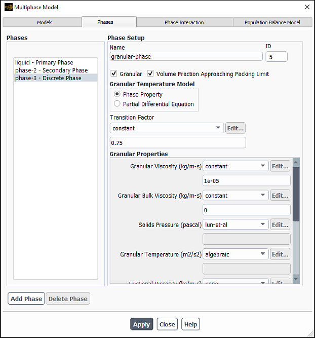
You can now define all other fields of the discrete phase in a similar manner to that described in Defining a Granular Secondary Phase.
If you are using the Eulerian multiphase model (Setting Up the Eulerian Model), you have the option of including the Boiling Model (see Wall Boiling Models in the Theory Guide).
Note the following limitations:
The boiling model is only available with
Eulerian multiphase model
Pressure-Based solver
Turbulent flow
The boiling model is not compatible with:
Species transport model
Standard moment, quadrature moment, and QMOM population balance methods
Simulations that involve granular secondary phases
The required work flow when using the boiling model is as follows:
Choose one of the turbulence models that is available with the Eulerian multiphase model.
Setup →
Models →
Viscous → Edit...
Open the Multiphase Model dialog box (Figure 26.83: The Boiling Model).
Setup →
Models →
Multiphase → Edit...
Enable Boiling Model in the Sub-Models group box.
Once the boiling model is enabled, Ansys Fluent automatically applies the default and recommended settings shown in the table below.
Parameter Setting Gravity Enabled Surface Tension Coefficient 0.07 N/m Drag Coefficient ishii Lift Coefficient tomiyama Secondary phase Diameter boiling-dia Mass transfer Mechanism for primary-secondary phase pairs boiling Heat Transfer Coefficient two-resistance Click Boiling Options..., and in the Boiling Options dialog box that opens (see Figure 26.84: The Boiling Options Dialog Box), you can select from the boiling model
- RPI Boiling Model
is where the total heat flux from the wall to the liquid is partitioned into three components, namely the convective heat flux, the quenching heat flux, and the evaporative heat flux. Details about this model can be found in RPI Model in the Theory Guide.
- Non-equilibrium Boiling
is a modification to the RPI model in order to model different boiling regimes like DNB and critical heat flux. Details about this model can be found in Non-equilibrium Subcooled Boiling in the Theory Guide.
- Critical Heat Flux
is where the critical heat flux condition is characterized by a sharp reduction of local heat transfer coefficients and the excursion of wall surface temperatures. Details about this model can be found in Critical Heat Flux in the Theory Guide.
Set the total Number of Eulerian Phases that are present in your case.
This can consist of two phases: liquid and vapor, which are directly involved in boiling mass transfer; or it can include “non-boiling phases” or “species“. If a system consists of three phases: liquid, vapor, and air, then the Number of Eulerian Phases will be
3, where air is the non-boiling phase.
Note:To include the liquid volume fraction effects, use the
solve/set/multiphase-numeric/boiling-parameters/liquid-vof-factortext command. When this option is enabled, the heat transfer coefficients of boiling models will be multiplied by the local liquid volume fraction.To include the thin film effects described in [86], use the
solve/set/multiphase-numeric/boiling-parameters/thin-filmtext command.
Make sure the energy option is enabled.
Note: The energy option will be automatically turned on when the boiling model is enabled.
Setup
→ Models → Energy On
Make sure that Gravity is enabled and set the Operating Pressure in the Operating Conditions dialog box.
Open the Create/Edit Materials dialog box and specify the material properties for the liquid, vapor, solid, and any other phases that may exist.
Setup →
Materials →
Fluid → Create/Edit...
Important: For the liquid and vapor phases, the Standard State Enthalpy must be specified, as it is used in the computation of the Latent Heat.
In the Phases tab, define the phases.
Define the liquid as the primary phase by selecting the phase from the Phases selection list that is labeled Primary Phase and specifying phase parameters in the Phase Setup group box.
Define the vapor as the secondary phase.
In the Multiphase Model dialog box, the Diameter is automatically set to boiling-dia by default, but you have the option of setting it up as a constant value or a user-defined function, as shown in Figure 26.85: The Multiphase Model Dialog Box for the Boiling Model (Phases Tab).
In the Phase Interaction > Forces tab, configure the following settings:
In the Drag Coefficient group box, you can select other than the default and recommended ishii drag specification method from the Coefficient drop-down list. See Specifying the Drag Function for available drag options and their definitions.
From the Lift Coefficient drop-down list, you can select other than the default tomiyama lift coefficient model as appropriate for your simulation (see Including the Lift Force for available options).
From the Wall Lubrication drop down list, select the wall lubrication model for your case (see Including the Wall Lubrication Force for details).
For boiling flows, antal-et-al is typically chosen.
From the Turbulent Dispersion drop-down list, select the turbulent dispersion force model (see Including the Turbulent Dispersion Force for details).
For boiling flows, lopez-de-bertodano is typically chosen. See Including the Turbulent Dispersion Force for details.
From the Turbulent Interaction drop-down list, select the desired turbulence correlation (see Including Turbulence Interaction Source Terms for details).
For boiling flows, troshko-hassan is typically chosen. See Including Turbulence Interaction Source Terms for details.
The default constant value of 0.07 N/m for the Surface Tension Coefficient is suitable for most cases. You can adjust the Surface Tension Coefficient if desired.
Click Apply.
In the Phase Interaction > Heat, Mass, Reactions > Mass tab, configure the following settings:
Specify the Number of Mass Transfer Mechanisms.
Make sure the transfer is always from the liquid to the vapor phase.
Make sure that boiling is selected under Mechanism.
In the Boiling Model dialog box that opens (Figure 26.87: The Boiling Model Dialog Box), set the following boiling model parameters and the quenching model corrections:
Specify the Interfacial Model Constants and the Saturation Temperature. The default values for the liquid and vapor interface transfer coefficients are 1.
Note:If you use the polynomial, piecewise-polynomial, or piecewise-linear option for Saturation Temperature, the pressure-dependency must be specified in terms of absolute pressure.
You may specify Saturation Temperature using RGP tables as described in Defining Saturation Properties via RGP Tables.
If you selected the Non-equilibrium Boiling or Critical Heat Flux in the Multiphase Model dialog box (Models tab), then you need to specify a value for the Vapor-Interface Transfer Coeff. parameter.
Under the Boiling Model Parameters, select the Bubble Departure Diameter that best describes your model from the following options:
tolubinski-kostanchuk (default, see Equation 14–518 in the Fluent Theory Guide)
unal (see Equation 14–520 in the Fluent Theory Guide)
kocamustafaogullari-ishii (see Equation 14–516 in the Fluent Theory Guide)
When you select kocamustafaogullari-ishii, the Kocamustafaogullari-Ishii Model Parameter dialog box opens automatically where you can adjust the value of the of the Bubble Contact Angle.
constant
user-defined
Specify the Frequency of Bubble Departure. You can choose the cole option (default, see Equation 14–514 in the Fluent Theory Guide), or enter a constant value.
Specify the Nucleation Site Density. You can choose between:
lemmert-chawla (default)
kocamustafaogullari-ishii
user-defined.
This quantity is usually represented by a correlation based on the wall superheat described in Equation 14–515 in the Theory Guide.
Note: It is recommended that when using the kocamustafaogullari-ishii option, it should be used for both the Bubble Departure Diameter and Nucleation Site Density.
Specify the Area Influence Coeff. The area of influence is based on the bubble departure diameter and the nucleate site density, as defined in Equation 14–511 in the Theory Guide. You can choose from the following options:
delvalle-kenning (default, see Equation 14–512 in the Fluent Theory Guide
constant
user-defined
If you have selected either the Non-equilibrium Boiling or Critical Heat Flux boiling option in the Multiphase Model dialog box (Models tab), you can select the Boiling Blending Function, which determines the partitioning of the wall heat flux between the liquid phase and the vapor phase, and specify its parameters. For more information, see Non-equilibrium Subcooled Boiling and Wall Heat Flux Partition in the Fluent Theory Guide
You can choose from the following options:
lavieville-et-al: Is the blending function by Lavieville et al. (see Equation 14–527 in the Fluent Theory Guide).
When you select lavieville-et-al, the Lavieville Model Parameters dialog box opens automatically where you can adjust the value of the Critical Liquid Volume Fraction (
 in Equation 14–527 in the Fluent Theory Guide).
tentner-et-al (default): Is the boiling blending function by Tentner et al. (see Equation 14–528 in the Fluent Theory Guide). This option is available only for the Critical Heat Flux boiling model.
When you select tentner-et-al, the Tentner Model Parameters dialog box opens automatically.
You can adjust the values of Vapor Volume Fraction Lower Limit and Vapor Volume Fraction Upper Limit (
 and
and  in Equation 14–528 in the Fluent Theory Guide, respectively).
ioilev-et-al: Is the boiling blending function by Ioilev et al. (see Equation 14–529 in the Fluent Theory Guide). This option is available only for the Critical Heat Flux boiling model.
The input parameters for the ioilev-et-al boiling bending function are similar to those for tentner-et-al. When you select ioilev-et-al, the Ioilev Model Parameters dialog box opens automatically where you can adjust the values of Vapor Volume Fraction Lower Limit and Vapor Volume Fraction Upper Limit (
 and
and  in Equation 14–529 in the Fluent Theory Guide, respectively)
user-defined: Allows you to implement and use your own boiling bending function using the
DEFINE_BOILING_PROPERTYuser-defined function (UDF). ReferDEFINE_BOILING_PROPERTYin the Fluent Customization Manual for details about this UDF.
If you use a mesh with y+ < 30, select NLBF Model in the Non-Local Boundary Field Model (NLBF) group box. This option helps prevent unphysical local temperature fields at the wall and achieve a less mesh dependent solution. This option is not compatible with the quenching model correction. If the Correction Model is enabled, you must disable it to use the NLBF Model.
The non-local boundary field (NLBF) model uses liquid temperatures from the bulk of the flow to determine the average temperature. This is done by collecting data from points on lines that are normal to the walls and extend into the interior of the domain. The points are equidistantly positioned on each line. The sampled temperature data is processed by the second order averaging algorithm that takes into account the temperature gradients and the sample point positions within relevant cells.
The average temperature is used in the calculations of quenching and bubble departure diameters.
You need to specify the following NLBF model parameters:
Maximum Line Length per Wall Element: Is the maximum value of the length of each line where the sampling points are located
Number of Points per Line: Is the number of the sample points on each line
Note:The points outside of the mesh are not accounted for in averaging the field data.
In dynamic mesh cases, the geometry of the mesh is automatically recalculated when mesh events occur.
When the calculation that involves the NLBF model is complete, an additional field variable called NLBF Averaged Temperature will be available for postprocessing under the Temperature... category at a mixture level.
In the Quenching Model Correction group box, specify the below settings. Note that the quenching model correction is not compatible with NLBF Model. If the NLBF Model is enabled, you must disable it to use the quenching model correction.
Quenching model correction addresses the quenching term in the wall heat flux partition (described in Wall Heat Flux Partition in the Theory Guide). The quenching term in the wall heat flux partition models the cyclic averaged transient energy transfer related to liquid filling the wall vicinity after the bubble detachment with a period
 and it is expressed as:
(26–23)
where
 is the liquid heat conductivity,
  is the periodic time,
  is a coefficient introduced to correct the waiting time
between departures of consecutive bubbles, and
is a coefficient introduced to correct the waiting time
between departures of consecutive bubbles, and  is the liquid phase diffusivity.
 From Equation 26–23, you can see that the quenching model is strongly dependent on
 , which results in grid-dependent solutions. To remedy this,
two approaches have been adopted in Ansys Fluent:
, which results in grid-dependent solutions. To remedy this,
two approaches have been adopted in Ansys Fluent: fixed y+ value
fixed liquid temperature
Note: When the calculated temperature in regions away from the walls is lower than the Operating Temperature (set in the Boussinesq Parameters group box in the Operating Conditions dialog box), the solver uses the operating temperature for the quenching correction.
Specify Bubble Waiting Time Coefficient, which is
in Equation 26–23. The default value is
1, however you can modify this value as needed, but it can only be
specified as a constant.Enable the Correction Model if you want to achieve a certain level of grid-independence in your solution. If this option is disabled, Equation 26–23 calculates the quench flux term without corrections.
Select Fixed Yplus Value if you want to use the logarithmic form of the wall functions to estimate the liquid temperature
 at a fixed Yplus value of 250, as proposed by Egorov and
Mentor [40], instead of using the liquid
temperature values in the near-wall cells. Enter the Minimum
Reference Temperature, which limits the lowest value of the
liquid temperature. It should not be lower than the liquid inlet
temperature. Specify a Yplus Value. It is set to 250
by default.
at a fixed Yplus value of 250, as proposed by Egorov and
Mentor [40], instead of using the liquid
temperature values in the near-wall cells. Enter the Minimum
Reference Temperature, which limits the lowest value of the
liquid temperature. It should not be lower than the liquid inlet
temperature. Specify a Yplus Value. It is set to 250
by default.If you select Fixed Liquid Temperature, you can choose from standard, constant, or user-defined for the Liquid Reference Temperature.
The standard method calculates the Liquid Reference Temperature as:

(26–24)

(26–25)

(26–26)
where
 = saturation temperature
 = intermediate temperature
 = average or bulk temperature of the liquid
 = vapor volume fraction
 and
and  = lower and upper limits for the vapor volume
fraction, equal to 0.05 and 0.3, respectively
= lower and upper limits for the vapor volume
fraction, equal to 0.05 and 0.3, respectively = linear blending function
You will also need to enter the Minimum Reference Temperature. The liquid temperature used to compute the quenching flux should usually be between the inlet liquid temperature and the saturation temperature.
Note: To learn how to hook boiling parameter user-defined functions, refer to
DEFINE_BOILING_PROPERTYin the Fluent Customization Manual.
Click Apply.
In the Phase Interaction > Heat, Mass, Reactions > Heat tab, specify the heat transfer coefficient for each phase pair. See Including Heat Transfer Effects for available options.
For cases with multiple boiling mechanisms (such as in boiling coupled with the inhomogeneous PBM), you can increase the robustness and accuracy of the solution by using the two-resistance boiling framework, which is invoked by the following text command:
solve/set/multiphase-numerics/heat-mass-transfer/boiling/two-resistance-boiling-framework?Allow generalized two-resistance framework for boiling? [no]yesOnce the generalized two-resistance boiling framework is enabled, the two resistance model with the default and recommended interphase heat transfer coefficients for the liquid and vapor phases is automatically assigned to each boiling phase pair. Note that with the two-resistance boiling framework, the only option that appears in the Heat Transfer Coefficient drop-down list for each boiling phase pair is two-resistance. You can modify the selection of the interphase heat transfer coefficient for the liquid phase in the Two Resistance Model dialog box.
For all other cases: Select the desired correlation from the Heat Transfer Coefficient drop-down box.
For boiling flows, ranz-marshall is usually chosen.
Click Apply.
In the Phase Interaction > Interfacial Area tab, configure the following settings:
For each phase pair, you can select from the following formulations:
ia-symmetric (see Equation 14–208 in the Theory Guide)
ia-particle (see Equation 14–207 in the Theory Guide)
ia-ishii (see Equation 14–211 in the Theory Guide). This option is only available with the RPI model.
user-defined (see Example 4- Custom Interfacial Area in the Fluent Customization Manual)
For boiling flows, ia-symmetric or ia-particle are usually chosen.
Click Apply.
Set up the conditions at inlets, outlets, and thermal conditions for walls.
Setup → Boundary
Conditions
The wall boiling models are compatible with three different wall boundaries: isothermal wall, specified heat flux, and specified heat transfer coefficient (coupled wall boundary).
Note: The boiling models do not apply to thin walls.
Choose Coupled as the pressure-velocity coupling scheme.
Solution →
Methods
Note: Although Phase Coupled SIMPLE is also available, it is generally less robust and is not recommended for use in steady cases involving boiling or mass transfer.
Adjust the solution controls for your simulation.
The following solution strategies are recommended for boiling model simulations:
Solution →
Controls
Courant Number: use a value between 1 and 20 is recommended. As a first try, use a value of 10.
Explicit Relaxation Factors: use the default values of 1 for Momentum and Pressure.
Vaporization Mass: use an under-relaxation factor between 0.5 and 1. As a first try, use a value of 1.
Volume Fraction: use an under-relaxation factor between 0.3 and 0.5.
Turbulent Kinetic Energy: use an under-relaxation factor between 0.3 and 0.8.
Turbulent Viscosity: use an under-relaxation factor between 0.5 and 1.0.
Energy: use an under-relaxation factor between 0.5 and 0.8.
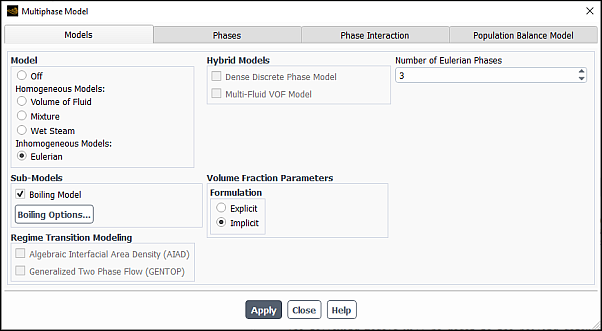
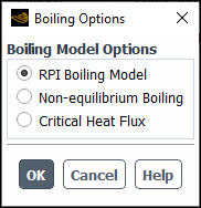
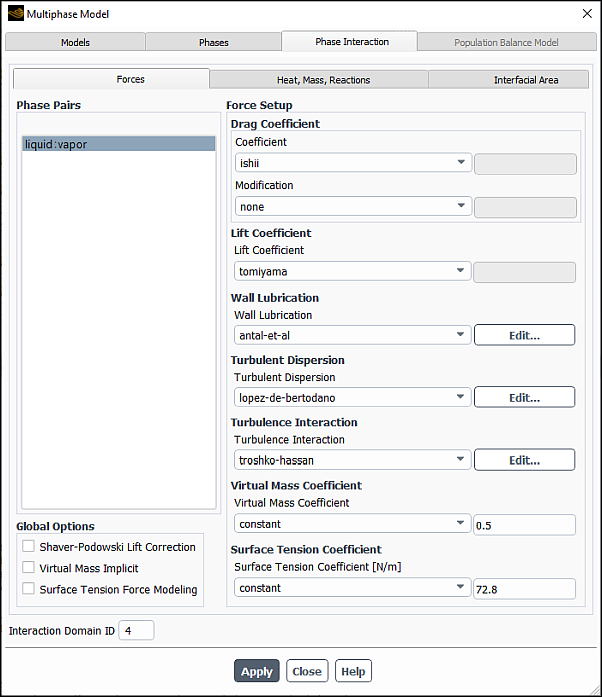
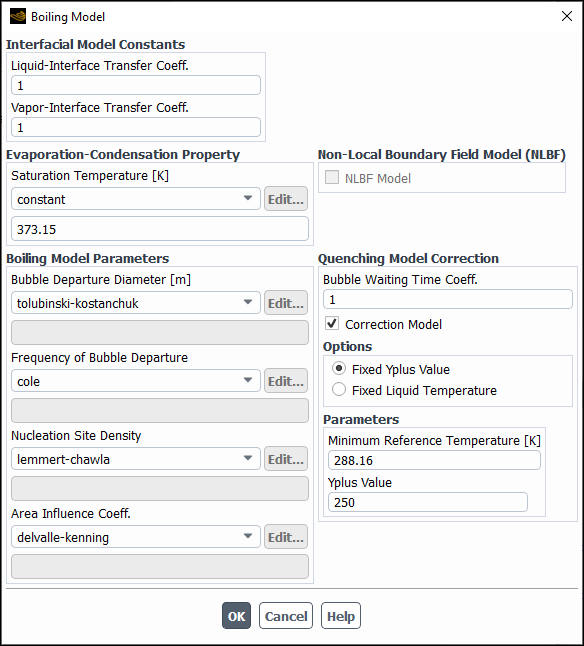
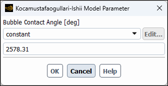
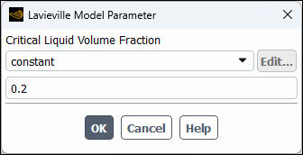
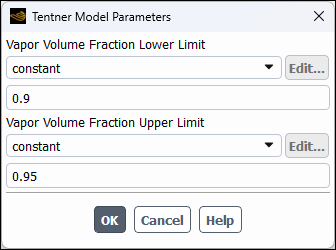
The following additional postprocessing variables are available in the Phase Interaction... category for generating contour plots for the mixture:
Saturation Temperature
Liquid Subcooling
Wall Superheat
Bubble Departure Diameter
Bubble Departure Frequency
Bubble Waiting Time
Bubble Area Fraction
Bubble Nucleation Site Density
With the exception of Saturation Temperature and Liquid Subcooling, these postprocessing variables are best visualized for heated walls. See Field Function Definitions for a complete list of field functions and their definitions.
The procedure for setting up a polydisperse boiling simulation is similar to that for setting up a boiling simulation outlined in Including the Boiling Model. Only the differences are highlighted here.
In the Models tab, set the total Number of Eulerian Phases to 3.
In the Phases tab, define, specify the liquid material as the primary phase, and the same vapor material as the secondary phases.
Important: Small and large bubbles formed during the boiling of the liquid phase will be designated to two separate secondary phases. Therefore, the material assigned to these two secondary phases must be identical.
In the Phase Interaction > Heat, Mass, Reactions > Mass tab, configure the following settings:
Set the Number of Mass Transfer Mechanisms to
2.Make sure the transfer is always from the liquid to the vapor phase.
For both phase pairs, select boiling under Mechanism.
Note: Although the bulk mass transfer (evaporation and condensation) is considered identical between the liquid and the two vapor phases, nucleation happens only for the phase which contains the smallest bin.
In the Population Balance Model tab, set up the population balance model (see Population Balance Model ) and configure the following settings.
Enable Phenomena.
Enable Nucleation Rate and Growth Rate.
Once these options are enabled, Ansys Fluent automatically selects the following options:
pb-boiling for both Nucleation Rate and Growth Rate
See Coupling Between the RPI Boiling Model and the Homogeneous or Inhomogeneous Discrete PBM in the Fluent Theory Guide for more information about the pb-boiling method.
sauter-mean for Diameter for both secondary phases (Phases tab)
This determines how the individual bin masses are distributed to ensure consistency of mass balance between phases and bins.
Optionally, enable and set up the aggregation and breakage kernels.
After you have selected the Eulerian multiphase model (Setting Up the Eulerian Model), you can enable the Multi-Fluid VOF Model (Multi-Fluid VOF Model in the Theory Guide).
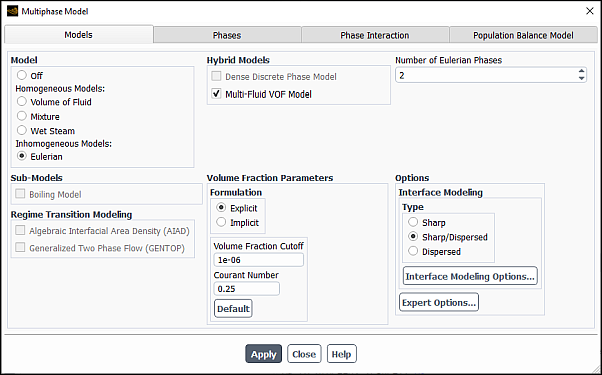
Note the following limitations:
This model is only available with the Eulerian multiphase model.
You cannot use this model with the Dense Discrete Phase Model.
After enabling Multi-Fluid VOF, the Interface Modeling Options become available, as described in Interface Modeling Type. You can select from Sharp, Dispersed, or hybrid Sharp/Dispersed interface modeling to expose the most appropriate discretization schemes for your simulation. You can also specify some additional time-advancement settings as described in Setting Time-Dependent Parameters for the Explicit Volume Fraction Formulation.
If you want to use the anisotropic drag law, perform the following steps:
Define the drag law in the Phase Interaction > Forces tab.
For each pair of phases, select the appropriate drag law from the Drag Coefficient drop-down list.
The available drag laws depend on your selection for Interface Modeling:
interface modeling supports only symmetric, anisotropic-drag, user-defined, and none.
Sharp/Dispersed interface modeling supports all the relevant drag laws described in Specifying the Drag Function.
Dispersed interface modeling does not support anisotropic-drag, but supports all other relevant drag laws (see Specifying the Drag Function).
With the and Sharp/Dispersed interface modeling, you can use anisotropic-drag when there is higher drag in the normal direction to the interface and lower drag in the tangential direction to the interface. For details about this drag law, refer to Multi-Fluid VOF Model in the Theory Guide.
Note: Anisotropic drag applicable to free surface modeling is only compatible with the Mixture turbulence model.
To specify the input parameters for anisotropic drag, you can use the
solve/set/mp-mfluid-aniso-dragtext command. The options for anAnisotropic Drag Methodof 0 (which is based on the symmetric drag), are as follows:Anisotropic Drag Method [0] Normal Interfacial Drag Friction Factor [1000000] Tangential Interfacial Drag Friction Factor [10] Length scale [0.0001]
The options for an
Anisotropic Drag Methodof 1 are as follows:Anisotropic Drag Method [0] 1 Viscosity option [2] Normal Interfacial Drag Friction Factor [1000000] Tangential Interfacial Drag Friction Factor [10] Length scale [0.0001]
Click Apply.
If you have enabled Phase Localized Discretization in the Models tab of the Multiphase Model dialog box, select the Phase Localized Compressive Scheme in the Discretization tab and click Apply to save your settings. For information about applying the various schemes, refer to Discretizing Using the Phase Localized Compressive Scheme.