Density weighted mean scalars (such as species fractions and temperature), denoted by , are calculated from the probability density function (PDF) of and as

(8–105)

Under the assumption of thin flames, so that only unburnt reactants and burnt products exist, the mean scalars are determined from

(8–106)

where the subscripts and denote burnt and unburnt, respectively.

The burnt scalars, , are functions of the mixture fraction and are calculated by mixing a mass of fuel with a mass of oxidizer and allowing the mixture to equilibrate. When non-adiabatic mixtures and/or diffusion laminar flamelets are considered, is also a function of enthalpy and/or strain, but this does not alter the basic formulation. The unburnt scalars, , are calculated similarly by mixing a mass of fuel with a mass of oxidizer, but the mixture is not reacted.

Just as in the non-premixed model, the chemistry calculations and PDF integrations for the burnt mixture are performed in Ansys Fluent, and look-up tables are constructed.

It is important to understand that in the limit of perfectly premixed combustion, the equivalence ratio and hence mixture fraction is constant. Hence, the mixture fraction variance and its scalar dissipation are zero. If you are using laminar diffusion flamelets, the flamelet at the lowest strain will always be interpolated, and if you have Include Equilibrium Flamelet enabled, the Ansys Fluent solution will be identical to a calculation with a chemical equilibrium PDF table.

The Laminar Flamelet model (see The Diffusion Flamelet Models Theory) postulates that a turbulent flame is an ensemble of laminar flames that have an internal structure not significantly altered by the turbulence. These laminar flamelets are embedded in the turbulent flame brush using statistical averaging. The Flamelet Generated Manifold (FGM) [666] model assumes that the scalar evolution (that is the realized trajectories on the thermochemical manifold) in a turbulent flame can be approximated by the scalar evolution in a laminar flame. Both Laminar Flamelet and FGM parameterize all species and temperature by a few variables, such as mixture-fraction, scalar-dissipation and/or reaction-progress, and solve transport equations for these parameters in a 3D CFD simulation.

Note that the FGM model is fundamentally different from the Laminar Flamelet model. For instance, since Laminar Flamelets are parameterized by strain, the thermochemistry always tends to chemical equilibrium as the strain rate decays towards the outlet of the combustor. In contrast, the FGM model is parameterized by reaction progress and the flame can be fully quenched, for example, by adding dilution air. No assumption of thin and intact flamelets is made by FGM, and the model can theoretically be applied to the stirred reactor limit, as well as to ignition and extinction modeling.

Any type of laminar flame can be used to parameterize an FGM. Ansys Fluent can either import an FGM calculated in a third-party flamelet code and written in Standard file format (see Standard Files for Flamelet Generated Manifold Modeling in the User's Guide), or calculate an FGM from 1D steady premixed flamelets or 1D diffusion flamelets.

In general, premixed FGMs should be used for turbulent partially-premixed flames that are predominantly premixed. Similarly, diffusion FGMs should be used for turbulent partially-premixed flames that are predominantly non-premixed. For further instructions on how to use the FGM model, see Flamelet Generated Manifold in the Fluent User's Guide.

 

8.3.2.2.1. Premixed FGMs in Reaction Progress Variable Space

While the only possible configuration for a diffusion flamelet in 1D is opposed flow, 1D steady premixed flamelets can have several configurations. These include unstrained adiabatic freely-propagating, unstrained non-adiabatic burner-stabilized, as well as a strained opposed flow premixed flames.

1D premixed flamelets can be solved in physical space (for example, [546], [97]), then transformed to reaction-progress space in the Ansys Fluent premixed flamelet file format, and imported into Ansys Fluent. Alternatively 1D premixed flamelets can be generated in Ansys Fluent, which solves the flamelets in reaction-progress space. The reaction progress variable is defined as a normalized sum of the product species mass fractions:

(8–107)

where
	superscript denotes the unburnt reactant at the flame inlet
	denotes the species mass fraction
	superscript denotes chemical equilibrium at the flame outlet
	are constants that are typically zero for reactants and unity for a few product species

The coefficients should be prescribed so that the reaction progress increases monotonically through the flame. By default, for all species other than , which are selected for hydrocarbon combustion. In the case where the element is missing from the chemical mechanism, such as combustion, Ansys Fluent uses for all species other than and , by default. For hydrogen blended fuels, the coefficients are defined based on the mass fraction of hydrogen in the fuel as:

where is the mass fraction of the hydrogen in the fuel composition. The coefficients can be specified in the user interface when generating FGM.

The 1D adiabatic premixed flame equations can be transformed from physical-space to reaction-progress space [477], [388]. Neglecting differential-diffusion, these equations are

(8–108)

(8–109)

where is the species mass fraction, is the temperature, is the fluid density, is time, is the species mass reaction rate, is the total enthalpy, and is the species specific heat at constant pressure.

The scalar-dissipation rate, in Equation 8–108 and Equation 8–109 is defined as

(8–110)

where is the thermal conductivity. Note that varies with and is an input to the equation set. If is taken from a 1D physical-space, adiabatic, equi-diffusivity flamelet calculation, either freely-propagating (unstrained) or opposed-flow (strained), the -space species and temperature distributions would be identical to the physical-space solution. However, is generally not known and is modeled in Ansys Fluent as

(8–111)

where is a user-specified maximum scalar dissipation within the premixed flamelet, and is the inverse complementary error function.

A 1D premixed flamelet is calculated at a single equivalence ratio, which can be directly related to a corresponding mixture fraction. For partially-premixed combustion, premixed laminar flamelets must be generated over a range of mixture fractions. Premixed flamelets at different mixture fractions have different maximum scalar dissipations, . In Ansys Fluent, the scalar dissipation at any mixture fraction is modeled as

(8–112)

where indicates stoichiometric mixture fraction.

Hence, the only model input to the premixed flamelet generator in Ansys Fluent is the scalar dissipation at stoichiometric mixture fraction, . The default value is 1/s, which reasonably matches solutions of unstrained (freely propagating) physical-space flamelets for rich, lean, and stoichiometric hydrocarbon and hydrogen flames at standard temperature and pressure.

The following are important points to consider about premixed flamelet generation in Ansys Fluent in general and when specifying in particular:

• It is common in the FGM approach to use unstrained, freely-propagating premixed flamelets. However, for highly turbulent flames where the instantaneous premixed flame front is stretched and distorted by the turbulence, a strained premixed flamelet may be a better representation of the manifold. The Ansys Fluent FGM model allows a premixed flamelet generated manifold at a single, representative strain rate, .

• Calculating flamelets in physical-space can be compute-intensive and difficult to converge over the entire mixture fraction range, especially with large kinetic mechanisms at the flammability limits. The Ansys Fluent solution in reaction-progress space is substantially faster and more robust than a corresponding physical-space solution. However, if physical-space solutions (for example, from [546], [97]) are preferred, they can be generated with an external code, transformed to reaction-progress space, and imported in Ansys Fluent's Standard Flamelet file format.

• A more appropriate value of than the default (1000/s) for the specific fuel and operating conditions of your combustor can be determined from a physical-space premixed flamelet solution at stoichiometric mixture fraction. This premixed flamelet solution can be unstrained or strained. through the flamelet is then calculated from Equation 8–110 and is the maximum value of .

• As is increased, the solution of temperature and species fractions as a function of tends to the thin-flamelet chemical equilibrium solution, which is linear between unburnt at and chemical equilibrium at . The minimum specified should be that in a freely-propagating flame. For smaller values of , the Ansys Fluent premixed flamelet generator will have difficulties converging. When Ansys Fluent fails to converge steady premixed flamelets at rich mixture fractions, equilibrium thin-flamelet solutions are used.

• The Ansys Fluent partially-premixed model can be used to model partially-premixed flames ranging from the non-premixed to the perfectly-premixed limit. In the non-premixed limit, reaction progress is unity everywhere in the domain and all premixed streams are fully burnt. In the premixed limit, the mixture fraction is constant in the domain. When creating a partially-premixed PDF table, the interface requires specification of the fuel and oxidizer compositions and temperatures. For partially-premixed flames, the fuel composition can be modeled as pure fuel, in which case any premixed inlet would be set to the corresponding mixture fraction, which is less than one. Alternatively, the fuel composition can be specified in the interface as a premixed inlet composition, containing both fuel and oxidizer components. In this latter case, the mixture fraction at premixed inlets would be set to one.

• You can use the automated grid refinement (AGR) when solving premixed flamelets. In the context of the FGM model, the grid in the reaction-progress space is refined. For information on the AGR, see Steady Diffusion Flamelet Automated Grid Refinement.

 

8.3.2.2.2. Premixed FGMs in Physical Space

The premixed FGM flamelets solved in reaction progress space using Equation 8–108 and Equation 8–109 require a closure of the scalar dissipation term. Ansys Fluent calculates the scalar dissipation in the progress variable using Equation 8–112, which is controlled by the following two parameters:

• Maximum value of the scalar dissipation for each mixture fraction

• Distribution of the scalar dissipation with respect to the reaction progress

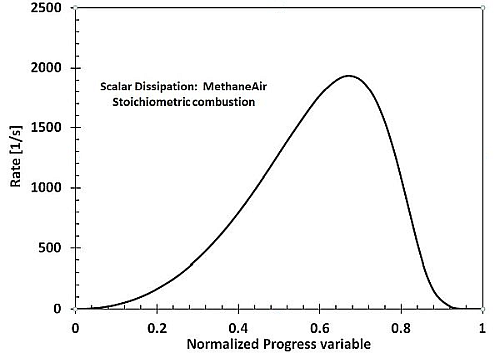
The maximum value of the scalar dissipation in Equation 8–112 is provided as a user input and is approximately calculated using the values of the flame thickness. The distribution of the scalar dissipation with respect to the reaction progress is modeled as a symmetric profile around the progress variable value c = 0.5 that decays exponentially towards the boundaries where c=0 or c =1.

Both approximations compromise the accuracy of the premixed FGM solution. If the flamelet equations are solved in the physical space, the scalar dissipation field is computed as part of the solution, and no assumption such as the shape of the scalar dissipation is made. Ansys Fluent allows you to generate the premixed FGM by solving flamelets in physical space using the Ansys Chemkin premixed flamelet generator. The governing equations and the method for solving laminar premixed flames are described in 1-D Premixed Laminar Flames in the Chemkin Theory Manual.

Figure 8.17: The Scalar Dissipation Rate Along The Normalized Reaction Progress Variable shows a distribution of the scalar dissipation for a stoichiometric methane air flamelet at 1 atm pressure calculated by the Ansys Chemkin premixed flamelet generator. The profile of the scalar dissipation exhibits an asymmetric peak distribution, which is consistent with the experimental results.

Figure 8.17: The Scalar Dissipation Rate Along The Normalized Reaction Progress Variable

The reaction progress variable is defined as a normalized fraction of product species (see Equation 8–107), namely . Note that the denominator, , is only a function of the local mixture fraction. When the Flamelet Generated Manifold model is enabled, Ansys Fluent solves a transport equation for the un-normalized progress variable, , and not the normalized progress variable, . This has two advantages. Firstly, since there are usually no products in the oxidizer stream, is zero and is undefined here (in other words, burnt air is the same as unburnt air). This can lead to difficulties in specifying oxidizer boundary conditions where oxidizer is mixed into unburnt reactants before the flame, as well as into burnt products behind the flame. Solving for avoids these issues and the solution is independent of the specified boundary value of for pure oxidizer inlets. The second advantage of solving for is that flame quenching can be modeled naturally. Consider a burnt stream in chemical equilibrium () that is rapidly quenched with an air jet. Since the equation in Ansys Fluent does not have a source term dependent on changes in mixture fraction, remains at unity and hence the diluted mixture remains at chemical equilibrium. Solving for can capture quenching since changes with mixture fraction, and the normalized reaction progress is correctly less than unity after mixing. To model these two effects with the normalized equation, additional terms involving derivatives and cross-derivatives of mixture fraction would be required [76]. However, these terms do not appear in the transport equation for the density-weighted un-normalized progress variable:

(8–113)

where is laminar thermal conductivity of the mixture, is the mixture specific heat.

Typically, in the FGM model, the mean source term is modeled as:

(8–114)

where is the joint PDF of reaction-progress () and mixture fraction (), and is the Finite-Rate flamelet source term from the flamelet library. Similar to Equation 8–88, the mean source term is multiplied by a wall damping constant at the wall boundaries. The default value of is unity.

The source term determines the turbulent flame position. Errors in both the approximation of the variance, as well as the assumed shape Beta PDF, can cause inaccurate flame positions.

Ansys Fluent has another option for modeling turbulence-chemistry interaction for the source term, in which the closure is based on the turbulent flame speed:

(8–115)

which is essentially the same source term when using the chemical equilibrium and diffusion flamelet partially-premixed models. An advantage of using a turbulent flame speed is that model constants can be calibrated to predict the correct flame position. In contrast, there are no direct parameters to control the FGM finite-rate source (Equation 8–114), and hence the flame position.

The joint PDF, in Equation 8–114, is specified as the product of two beta PDFs. The beta PDFs require second moments (that is, variances). The variance of the un-normalized reaction progress variable is modeled either with a transport equation

(8–116)

where ,

or with an algebraic expression

(8–117)

where is the turbulence length scale and is a constant with a default value of 0.1.

For the SBES turbulence model, a blending formulation is used for the variance of the un-normalized reaction progress variable in the following way:

(8–118)

where subscripts and correspond to the RANS and LES modeling regions, respectively, and is the shielding function defined in Equation 4–297.

 

8.3.2.3.1. Scalar Transport with FGM Closure

In the FGM model, the species concentration is obtained from reduced variables, such as the mixture fraction, progress variable, and their variances. Since the definition of the progress variable is predominantly based on the global species, the progress variable tracks the evolution of the major species and heat release reactions. In a reacting mixture, however, not all species evolve at the same rate due to the differences in their time scales. For example, the global progress variable may approach the unity, which marks the completion of a reaction. Meanwhile, a slow forming species, such as nitric oxide NO, may still be evolving. Therefore, mapping that is performed solely on the basis of the global progress variable may lead to inaccurate results for the slow-forming species.

The progress variable is a reduced-order modeling approach that is based on a representative time scale of a reacting mixture. In reality, different species within a reacting mixture may have large disparities in their reaction time scales. Reduced-order models cannot capture these disparities. Solving for multiple separate transport equations for slow-forming species is one of the alternative approaches that will account for differences in the time scales of species evolution. Within the framework of the FGM model, Ansys Fluent provides an option to solve generic transport scalar equations, in addition to the global progress variable equation. These generic scalar transport equations can be solved for minor species that are low in concentration and, therefore, have no feedback on the main flow field, and that have time scales much slower than those of the major species in the mixture.

The transport equation of a generic scalar solved with the FGM model in Ansys Fluent has the following form:

(8–119)

In this equation, the scalar that is to be transported can be a mass fraction of any species in the mixture. The last term is the reaction source term. It represents the net production rate of the scalar and is computed as the difference between its forward reaction rates and revere reaction rates.

The forward reaction rates of the scalar are not dependent on the value of . Therefore, they can be pre-tabulated and stored in the PDF table. On the other hand, the reverse reaction rates of the scalar are dependent on the concentration of . Therefore, the pre-tabulated values for the reverse reaction rates need to be corrected based on the solved transport scalar equation [268].

In Ansys Fluent, the reverse reaction rates are first calculated using the prevailing values of the scalar , and then they are stored in the PDF table. At the run time, the reverse reaction rates are scaled using the value of the solved transport scalar in the following way:

(8–120)

where and are the forward and revere reaction rates, respectively, and is an averaged value of the transported scalar stored in the PDF table. This methodology allows the consumption of the scalar to respond to the slow evolution of the scalar solved.

The scalar transport model assumes that all the species, except for those solved as scalars, will occur over relatively short time scales. The scalar solved in Equation 8–119 is treated as a passive scalar, with no impact on the flow field, temperature, or mixture properties. Therefore, the scalar transport option should be used only for species that are low in concentration and that also have a slow formation rate. A typical example of such a species (for which a mass fraction can be solved as a scalar) is nitric oxide (NO). In the case of multiple scalar equations, the scalar equation for each species is solved independently, and the concentration of the remaining species is taken from the PDF tables.

---

Note:  The scalar equations are treated as passive scalars that do not provide feedback to the flow equations or mixture properties. Therefore, for steady-state simulations, these equations can be solved in a post-processing mode, as for example, when modeling pollutant formation in Ansys Fluent.

---

The flamelets generated using the premixed or diffusion FGM model store instantaneous species mass fractions and temperature as a function of the local mixture fraction and the progress variable . The mean thermochemical properties of the mixture are determined by averaging the instantaneous thermochemical property values using the modeled PDF as:

(8–121)

where denotes the species mass fraction or temperature from the flamelet files. In addition to temperature and species mass fraction, other mixture properties, such as specific heat, density, and molecular weight, can also be evaluated using Equation 8–121. The average mixture properties for an adiabatic system are represented as a function of mean mixture fraction , mean progress variable , and their variances and and are stored inside a four-dimensional PDF table:

(8–122)

Non-adiabatic Extension for Average Mixture Properties Calculation

Similar to Non-Adiabatic Extensions of the Non-Premixed Model, the fluctuations of enthalpy are ignored with the non-adiabatic extension to the PDF model. The average mixture properties for non-adiabatic partially premixed combustion using FGM can then be calculated as:

(8–123)

where is the mean enthalpy.

For non-adiabatic systems, each of the average mixture properties is a function of five independent variables:

(8–124)

Calculation of average mixture properties using Equation 8–123 and Equation 8–124 requires a five-dimensional PDF table, which places an enormous demand on memory and could be computationally expensive. In order to optimize the run-time memory requirements and computational cost, the non-adiabatic PDF tables are generated with the following assumptions:

With these assumptions, the average species mass fraction and, therefore, molecular weight can be calculated using Equation 8–122, ignoring the enthalpy level. The other mixture properties, such as temperature, specific heat, and density, account for the enthalpy changes and are estimated as:

(8–125)

(8–126)

For FGM models, all properties, burnt or unburnt, are computed from the PDF tables as described in Equation 8–125 and Equation 8–126. However, for non-FGM models, unburnt properties are computed as described in this section.

Turbulent fluctuations are neglected for the unburnt mixture, so the mean unburnt scalars, , are functions of only. The unburnt density, temperature, specific heat, and thermal diffusivity are fitted in Ansys Fluent to third-order polynomials of using linear least squares:

(8–127)

Since the unburnt scalars are smooth and slowly-varying functions of , these polynomial fits are generally accurate. Access to polynomials is provided in case you want to modify them.

When the secondary mixture fraction model is enabled, the unburnt density, temperature, specific heat, thermal diffusivity, and laminar flame speed are calculated as follows: polynomial functions are calculated for a mixture of pure primary fuel and oxidizer, as described above, and are a function of the mean primary mixture fraction, . Similar polynomial functions are calculated for a mixture of pure secondary fuel and oxidizer, and are a function of the normalized secondary mixture fraction, . The unburnt properties in a cell are then calculated as a weighted function of the mean primary mixture fraction and mean secondary normalized mixture fraction as,

(8–128)

The premixed models require the laminar flame speed (see Equation 8–77), which depends strongly on the composition, temperature, and pressure of the unburnt mixture. For adiabatic perfectly premixed systems as in Premixed Combustion, the reactant stream has one composition, and the laminar flame speed is constant throughout the domain. However, in partially premixed systems, the laminar flame speed will change as the reactant composition (equivalence ratio) changes, and this must be taken into account.

Accurate laminar flame speeds are difficult to determine analytically, and are usually measured from experiments or computed from 1D simulations. For the partially-premixed model, in addition to the laminar flame speed model options described in Laminar Flame Speed, namely constant, user-defined function, and Metghalchi-Keck, Ansys Fluent offers the following methods:

For all these methods, Ansys Fluent fits the curves to a piecewise-linear polynomial. Mixtures leaner than the lean limit or richer than the rich limit will not burn and have zero flame speed. The required inputs are values for the laminar flame speed at 20 mixture fraction () points.

For non-adiabatic simulations, such as heat transfer at walls or compressive heating, the unburnt mixture temperature may deviate from its adiabatic value. The piecewise-linear function of mixture fraction is unable to account for this effect on the laminar flame speed. You can include non-adiabatic effects on the laminar flame speed by enabling Non-Adiabatic Laminar Flame Speed, which tabulates the laminar speeds in the PDF table by evaluating the curve fits from [216] at the enthalpy levels in the PDF table. Note that the tabulated mean laminar flame speed accounts for fluctuations in the mixture fraction.

In the Flamelet Generated Manifold (FGM) model, the reaction source term for the progress variable equation can be modeled using either the finite rate source as in Equation 8–114 or the turbulent flame speed closure as in Equation 8–115. When the turbulent flame speed closure is employed, Ansys Fluent tabulates the laminar flame speed using either prepdf polynomials or the flame speed library as described in Laminar Flame Speed. The flame speed computed from different methods described in Laminar Flame Speed is obtained by solving one-dimensional premixed freely propagating flame configurations. The flame speed is then expressed as a polynomial function of the mixture fraction.

In most practical combustion systems, the flames experience strain due to various factors such as turbulence, swirl, geometry, and so on. The impact of the strain rate on the flame can be neglected for a wide range of applications, and, therefore, the flame speed can be computed using the freely propagating flames with reasonable accuracy. However, the impact of the strain on the flame is magnified in certain scenarios such as the lean blow-off limit, highly swirling flames with lean premixed conditions, and so on. For these applications, using the unstrained flame speed can often over-predict the flame speed and may lead to inaccurate prediction of critical combustion characteristics. In such cases, the accuracy of the combustion modeling can be improved if the impact of the strain rate on the flame speed is taken into account.

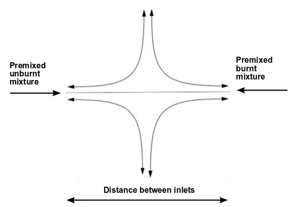
Such effects are considered in the strained flame speed model in Ansys Fluent. In this model, the strained flame speed is tabulated as a function of the strain rate and mixture fraction. For each strain rate and mixture fraction, the strained flame speed is calculated using one-dimensional premixed opposed-flow strained flamelets. The computational domain of this configuration contains two opposed-flow inlets and one-dimensional solution domain in physical space. The configuration schematics for flamelet generation is shown in Figure 8.18: Premix Opposed Flow Configuration for the Strained Flame Speed.

Figure 8.18: Premix Opposed Flow Configuration for the Strained Flame Speed

The premixed opposed-flow strained flamelets are solved in physical space using the Ansys Chemkin Oppdif solver. The details of the Oppdif solver are provided in Opposed-flow and Stagnation Flames in the Chemkin Theory Manual.

The strained flamelets use the following boundary conditions for the two inlets:

Flamelet Generation and Flame Speed Calculations

The strain rate (1/s) is computed as

(8–129)

where

= burning rate of fuel

= velocity at the unburnt mixture inlet

= distance between the two inlets

If both inlet jets have equal momentum, then

(8–130)

where and are the densities of the unburnt and burnt mixtures, respectively.

From Equation 8–129 and Equation 8–130, the strain rate can be obtained as:

(8–131)

The strained flamelets are generated to increase the strain rate to its maximum value. For a given strain rate, both inlet velocities are computed using Equation 8–130 and Equation 8–131. The strained flame speed for a given mixture fraction and strain rate is computed as:

(8–132)

where is the burning rate of fuel, and is the mass fraction of the fuel. Prior to the CFD solution, the strained flame speed is computed as a function of the strain rate and mixture fraction and stored as a table.

During the CFD solution, the strained flame speed is interpolated as a function of the mixture fraction and computed strain rate using the stored data. It is then used in the turbulent flame speed closure in Equation 8–115:

Strain Rate Calculation in the CFD Solution

The solution of the strained flamelets is used to compute the strained flame speed, which is tabulated as a function of the strain rate and mixture fraction. The mixture fraction is obtained from the solution of the transport equation as described in Premixed FGMs in Physical Space. The total strain rate in the CFD solution is computed using the local flow conditions as a sum of the strain rate due to mean flow and due to turbulence [646]:

(8–133)

where the strain rate due to mean flow is computed as:

(8–134)

and the strain rate due to the turbulent flow is modeled as [118]:

(8–135)

In the above equations,

= flow velocity in the control volume

= unit normal to the flame surface; , where is the progress variable

= turbulent dissipation rate

= turbulent kinetic energy

= intermediate turbulent net flame stretch (ITNFS) term

= user-speecified coefficient that determines the weight of the term relative to a straightforward turbulent time scale (default = 1)

For RANS-based turbulence models, =1.

For LES models, is computed as:

(8–136)

with

(8–137)

and

(8–138)

In Equation 8–136 thru Equation 8–138, the following notations are used:

= turbulent velocity fluctuation

= laminar flame speed

= integral turbulent length scale

= laminar flame thickness

 

8.3.2.7.1. Strained Non-Adiabatic Flame Speed

Many combustion devices involve significant heat loss through the walls. In such cases, the flame speed is not only dependent on the strain rate, but also sensitive to the heat loss. To account for the impact of heat loss on strained flamelets, Ansys Fluent provides a non-adiabatic extension of the strained flame speed. In this approach, the flame speed is computed using the premixed opposed flow configuration (see Figure 8.18: Premix Opposed Flow Configuration for the Strained Flame Speed) with a different heat loss parameter applied on the premixed burnt mixture side inlet.

The heat loss is caused by cooling the burned products, and the heat loss parameter is defined as:

(8–139)

where is the temperature achieved by cooling the burned products, and is the temperature of the premixed burnt mixture without any heat loss.

For the non-adiabatic strained flame speed calculation, the strained flamelets are generated for different levels of the heat loss parameter. =0 corresponds to no heat loss, and therefore gives the strained adiabatic flame speed. The non-adiabatic strained flame speed is stored in a three-dimensional table as a function of the mixture fraction (), strain rate (), and heat loss parameter ():

(8–140)

During the CFD solution, the heat loss parameter () is calculated for each cell volume as a ratio of temperatures for cell enthalpy () and adiabatic enthalpy () obtained for the same mixture fraction () and progress variable ():

(8–141)

The strained flame speed from the PDF table is then interpolated using the mixture fraction (), strain rate () and cell heat loss parameter ().

In both the diffusion and premixed FGM models, the automated grid refinement (AGR) can be used for generating the PDF lookup table. For further details about AGR, see Generating Lookup Tables Through Automated Grid Refinement. In the current implementation, the grid points used in the mixture fraction and reaction-progress space are fixed, and they are taken from the flamelet calculation. The grid refinement procedure is conducted in the mixture fraction variance, reaction progress variance, and mean enthalpy space.