


The discrete ordinates (DO) radiation model solves the radiative
transfer equation (RTE) for a finite number of discrete solid angles,
each associated with a vector direction  fixed in the global
Cartesian system (
fixed in the global
Cartesian system ( ). You control the fineness of the angular discretization,
analogous to choosing the number of rays for the DTRM. Unlike the
DTRM, however, the DO model does not perform ray tracing. Instead,
the DO model transforms Equation 5–22 into a transport
equation for radiation intensity in the spatial coordinates (
). You control the fineness of the angular discretization,
analogous to choosing the number of rays for the DTRM. Unlike the
DTRM, however, the DO model does not perform ray tracing. Instead,
the DO model transforms Equation 5–22 into a transport
equation for radiation intensity in the spatial coordinates ( ). The DO model solves for as many transport equations
as there are directions
). The DO model solves for as many transport equations
as there are directions  . The solution method is identical
to that used for the fluid flow and energy equations.
. The solution method is identical
to that used for the fluid flow and energy equations.
Two implementations of the DO model are available in Ansys Fluent: uncoupled and (energy) coupled. The uncoupled implementation is sequential in nature and uses a conservative variant of the DO model called the finite-volume scheme [110], [538], and its extension to unstructured meshes [466]. In the uncoupled case, the equations for the energy and radiation intensities are solved one by one, assuming prevailing values for other variables.
Alternatively, in the coupled ordinates method (or COMET) [415], the discrete energy and intensity equations at each cell are solved simultaneously, assuming that spatial neighbors are known. The advantages of using the coupled approach is that it speeds up applications involving high optical thicknesses and/or high scattering coefficients. Such applications slow down convergence drastically when the sequential approach is used. For information about setting up the model, see Setting Up the DO Model in the User’s Guide.
The DO model considers the radiative transfer equation (RTE)
in the direction  as a field equation. Thus, Equation 5–22 is written as
 | (5–64) |
Ansys Fluent also allows the modeling of non-gray radiation
using a gray-band model. The RTE for the spectral intensity  can be written as [[448] equation 9.22]
 | (5–65) |
Here  is the wavelength,
  is the spectral
absorption coefficient, and
is the spectral
absorption coefficient, and  is the black
body intensity given by the Planck function. The scattering coefficient,
the scattering phase function, and the refractive index
is the black
body intensity given by the Planck function. The scattering coefficient,
the scattering phase function, and the refractive index  are assumed independent
of wavelength.
are assumed independent
of wavelength.
The non-gray DO implementation divides the radiation spectrum
into  wavelength bands, which need not be contiguous or
equal in extent. The wavelength intervals are supplied by you, and
correspond to values in vacuum (
wavelength bands, which need not be contiguous or
equal in extent. The wavelength intervals are supplied by you, and
correspond to values in vacuum ( ). The RTE is integrated over
each wavelength interval, resulting in transport equations for the
quantity
). The RTE is integrated over
each wavelength interval, resulting in transport equations for the
quantity  , the radiant
energy contained in the wavelength band
, the radiant
energy contained in the wavelength band  . The behavior
in each band is assumed gray. The black body emission in the wavelength
band per unit solid angle is written as
. The behavior
in each band is assumed gray. The black body emission in the wavelength
band per unit solid angle is written as
 | (5–66) |
where  is the
fraction of radiant energy emitted by a black body [447] in the wavelength interval from 0 to
is the
fraction of radiant energy emitted by a black body [447] in the wavelength interval from 0 to  at temperature
  in a medium of refractive
index
in a medium of refractive
index  .
.  and
and  are the wavelength boundaries of the band.
The total intensity  in each
direction
in each
direction  at position
  is computed using
 | (5–67) |
where the summation is over the wavelength bands.
Boundary conditions for the non-gray DO model are applied on a band basis. The treatment within a band is the same as that for the gray DO model.
The coupling between energy and radiation intensities at a cell (which is also known as COMET) [415] accelerates the convergence of the finite volume scheme for radiative heat transfer. This method results in significant improvement in the convergence for applications involving optical thicknesses greater than 10. This is typically encountered in glass-melting applications. This feature is advantageous when scattering is significant, resulting in strong coupling between directional radiation intensities. This DO model implementation is utilized in Ansys Fluent by enabling the DO/Energy Coupling option for the DO model in the Radiation Model dialog box. The discrete energy equations for the coupled method are presented below.
The energy equation when integrated over a control volume  , yields the discrete energy
equation:
, yields the discrete energy
equation:
 | (5–68) |
|
where | |
|
| |
|
| |
|
| |
|
| |
|
|


The coefficient  and the source term
  are due to the discretization
of the convection and diffusion terms as well as the non-radiative
source terms.
are due to the discretization
of the convection and diffusion terms as well as the non-radiative
source terms.
Combining the discretized form of Equation 5–64 and the discretized energy equation, Equation 5–68, yields [415]:
 | (5–69) |
where
 | (5–70) |
 | (5–71) |
 | (5–72) |
There are some instances when using DO/Energy coupling is not recommended or is incompatible with certain models:
DO/Energy coupling is not recommended for cases with weak coupling between energy and directional radiation intensities. This may result in slower convergence of the coupled approach compared to the sequential approach.
DO/Energy coupling is not available when solving enthalpy equations instead of temperature equations. Specifically, DO/Energy coupling is not compatible with the non-premixed or partially premixed combustion models.
To find out how to apply DO/Energy coupling, refer to Setting Up the DO Model in the User's Guide.
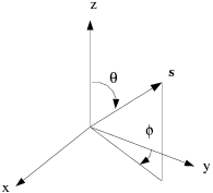
Each octant of the angular space  at any spatial
location is discretized into
at any spatial
location is discretized into  solid
angles of extent
solid
angles of extent  , called control angles.
The angles
, called control angles.
The angles  and
and  are the polar and azimuthal angles respectively,
and are measured with respect to the global Cartesian system
are the polar and azimuthal angles respectively,
and are measured with respect to the global Cartesian system  as shown in Figure 5.3: Angular Coordinate System. The
  and
and  extents of the control angle,
  and
and  ,
are constant. In two-dimensional calculations, only four octants are
solved due to symmetry, making a total of
,
are constant. In two-dimensional calculations, only four octants are
solved due to symmetry, making a total of  directions in all. In three-dimensional calculations,
a total of
directions in all. In three-dimensional calculations,
a total of  directions
are solved. In the case of the non-gray model,
directions
are solved. In the case of the non-gray model,  or
or  equations
are solved for each band.
equations
are solved for each band.
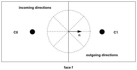
When Cartesian meshes are used, it is possible to align the global angular discretization with the control volume face, as shown in Figure 5.4: Face with No Control Angle Overhang. For generalized unstructured meshes, however, control volume faces do not in general align with the global angular discretization, as shown in Figure 5.5: Face with Control Angle Overhang, leading to the problem of control angle overhang [466].
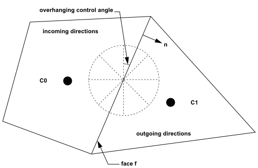
Essentially, control angles can straddle the control volume faces, so that they are partially incoming and partially outgoing to the face. Figure 5.6: Face with Control Angle Overhang (3D) shows a 3D example of a face with control angle overhang.
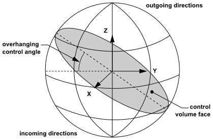
The control volume face cuts the sphere representing the angular space at an arbitrary angle. The line of intersection is a great circle. Control angle overhang may also occur as a result of reflection and refraction. It is important in these cases to correctly account for the overhanging fraction. This is done through the use of pixelation [466].
Each overhanging control angle is divided into  pixels, as shown in Figure 5.7: Pixelation of Control Angle.
The energy contained in each pixel is then treated as incoming
or outgoing to the face. The influence of overhang can therefore be
accounted for within the pixel resolution. Ansys Fluent allows you
to choose the pixel resolution. For problems involving gray-diffuse
radiation, the default pixelation of  is usually
sufficient. For problems involving symmetry, periodic, specular, or
semi-transparent boundaries, a pixelation of
is usually
sufficient. For problems involving symmetry, periodic, specular, or
semi-transparent boundaries, a pixelation of  is recommended.
You should be aware, however, that increasing the pixelation adds
to the cost of computation.
is recommended.
You should be aware, however, that increasing the pixelation adds
to the cost of computation.
The DO implementation in Ansys Fluent admits a variety of scattering phase functions. You can choose an isotropic phase function, a linear anisotropic phase function, a Delta-Eddington phase function, or a user-defined phase function. The linear anisotropic phase function is described in Equation 5–33. The Delta-Eddington function takes the following form:
 | (5–73) |
Here,  is the forward-scattering factor and
  is the Dirac delta function. The
  term essentially cancels
a fraction
term essentially cancels
a fraction  of the out-scattering; therefore, for
  , the Delta-Eddington
phase function will cause the intensity to behave as if there is no
scattering at all.
, the Delta-Eddington
phase function will cause the intensity to behave as if there is no
scattering at all.  is the asymmetry factor. When the Delta-Eddington
phase function is used, you will specify values for
is the asymmetry factor. When the Delta-Eddington
phase function is used, you will specify values for  and
and  .
.
When a user-defined function is used to specify the scattering phase function, Ansys Fluent assumes the phase function to be of the form
 | (5–74) |
The user-defined function will specify  and the forward-scattering factor
  .
.
The scattering phase functions available for gray radiation can also be used for non-gray radiation. However, the scattered energy is restricted to stay within the band.
The DO model allows you to include the effect of a discrete second phase of particulates on radiation. In this case, Ansys Fluent will neglect all other sources of scattering in the gas phase.
The contribution of the particulate phase appears in the RTE as:
 | (5–75) |
where  is the equivalent absorption
coefficient due to the presence of particulates, and is given by Equation 5–36. The equivalent emission
is the equivalent absorption
coefficient due to the presence of particulates, and is given by Equation 5–36. The equivalent emission
 is given by Equation 5–35. The equivalent particle scattering
factor
is given by Equation 5–35. The equivalent particle scattering
factor  , defined in Equation 5–39, is used in the scattering terms.
For non-gray radiation, absorption, emission, and scattering due to the particulate phase are included in each wavelength band for the radiation calculation. Particulate emission and absorption terms are also included in the energy equation.
The discrete ordinates radiation model allows the specification of opaque walls that are interior to a domain (with adjacent fluid or solid zones on both sides of the wall), or external to the domain (with an adjacent fluid or solid zone on one side, only). Opaque walls are treated as gray if gray radiation is being computed, or non-gray if the non-gray DO model is being used.
Figure 5.8: DO Radiation on Opaque Wall shows a schematic of radiation on an opaque wall in Ansys Fluent.
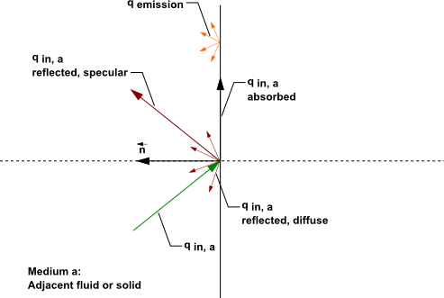
The diagram in Figure 5.8: DO Radiation on Opaque Wall
shows incident radiation  on side
 a of an opaque wall. Some of the radiant energy is reflected
diffusely and specularly, depending on the diffuse fraction  for side
 a of the wall that you specify as a boundary condition.
Some of the incident radiation is absorbed at the surface of the wall and some radiation is emitted from the wall surface as shown in Figure 5.8: DO Radiation on Opaque Wall. The amount of incident radiation absorbed at the wall surface and the amount emitted back depends on the emissivity of that surface and the diffuse fraction. For non-gray DO models, you must specify internal emissivity for each wavelength band. Radiation is not transmitted through an opaque wall.
Radiant incident energy that impacts an opaque wall can be reflected
back to the surrounding medium and absorbed by the wall. The radiation
that is reflected can be diffusely reflected and/or specularly reflected,
depending on the diffuse fraction  . If
. If  is the amount of radiative energy incident on the
opaque wall, then the following general quantities are computed by Ansys Fluent for opaque walls:
is the amount of radiative energy incident on the
opaque wall, then the following general quantities are computed by Ansys Fluent for opaque walls:
emission from the wall surface

diffusely reflected energy

specularly reflected energy

absorption at the wall surface

where  is the diffuse fraction,
  is the refractive index
of the adjacent medium,
is the refractive index
of the adjacent medium,  is the wall emissivity,
  is the Stefan-Boltzmann
Constant, and
is the Stefan-Boltzmann
Constant, and  is the wall temperature.
Note that although Ansys Fluent uses emissivity in its computation
of radiation quantities, it is not available for postprocessing. Absorption
at the wall surface assumes that the absorptivity is equal to the
emissivity. For a purely diffused wall,  is equal to
  and there is no specularly
reflected energy. Similarly, for a purely specular wall,
and there is no specularly
reflected energy. Similarly, for a purely specular wall,  is equal to
  and there is no diffusely
reflected energy. A diffuse fraction between
and there is no diffusely
reflected energy. A diffuse fraction between  and
and  will result in partially diffuse
and partially reflected energy.
will result in partially diffuse
and partially reflected energy.
For gray diffuse radiation, the incident radiative heat flux,  , at the wall is
The net radiative flux leaving the surface is given by
 | (5–76) |
 | (5–77) |
|
where | |
|
| |
|
| |
|
| |
|
|


This equation is also valid for specular radiation with emissivity
=  .
.
The boundary intensity for all outgoing directions  at the wall is given by
 | (5–78) |
There is a special set of equations that apply uniquely to non-gray
diffuse opaque walls. These equations assume that the absorptivity
is equal to the emissivity for the wall surface. For non-gray diffuse
radiation, the incident radiative heat flux  in the band
  at
the wall is
at
the wall is
 | (5–79) |
The net radiative flux leaving the surface in the band  is
given by
is
given by
 | (5–80) |
where  is
the wall emissivity in the band.
is
the wall emissivity in the band.  provides the Planck distribution function.
This defines the emittance for each radiation band as a function of
the temperature of the source surface. The boundary intensity for
all outgoing directions
provides the Planck distribution function.
This defines the emittance for each radiation band as a function of
the temperature of the source surface. The boundary intensity for
all outgoing directions  in the band
  at
the wall is given by
at
the wall is given by
 | (5–81) |
Ansys Fluent allows the specification of interior and exterior semi-transparent walls for the DO model. In the case of interior semi-transparent walls, incident radiation can pass through the wall and be transmitted to the adjacent medium (and possibly refracted), it can be reflected back into the surrounding medium, and absorbed through the wall thickness. Transmission and reflection can be diffuse and/or specular. You specify the diffuse fraction for all transmitted and reflected radiation; the rest is treated specularly. For exterior semi-transparent walls, there are two possible sources of radiation on the boundary wall: an irradiation beam from outside the computational domain and incident radiation from cells in adjacent fluid or solid zones.
For non-gray radiation, semi-transparent wall boundary conditions are applied on a per-band basis. The radiant energy within a band is transmitted, reflected, and refracted as in the gray case; there is no transmission, reflection, or refraction of radiant energy from one band to another.
By default the DO equations are solved in all fluid zones, but not in any solid zones. Therefore, if you have an adjacent solid zone for your thin wall, you will need to specify the solid zone as participating in radiation in the Solid dialog box as part of the boundary condition setup.
Important: If you are interested in the detailed temperature distribution inside your semi-transparent media, then you will need to model a semi-transparent wall as a solid zone with adjacent fluid zone(s), and treat the solid as a semi-transparent medium. This is discussed in a subsequent section.
Figure 5.9: DO Radiation on Interior Semi-Transparent Wall shows a schematic
of an interior (two-sided) wall that is treated as semi-transparent
in Ansys Fluent and has zero-thickness. Incident radiant energy depicted
by  can pass through the
semi-transparent wall if and only if the contiguous fluid or solid
cell zones participate in radiation, thereby allowing the radiation
to be coupled. Radiation coupling is set when a wall is specified
as semi-transparent. Note that by default, radiation is not coupled and you will need to explicitly specify radiation
coupling on the interior wall by changing the boundary condition type
to semi-transparent in the Wall dialog box (under
the Radiation tab).
can pass through the
semi-transparent wall if and only if the contiguous fluid or solid
cell zones participate in radiation, thereby allowing the radiation
to be coupled. Radiation coupling is set when a wall is specified
as semi-transparent. Note that by default, radiation is not coupled and you will need to explicitly specify radiation
coupling on the interior wall by changing the boundary condition type
to semi-transparent in the Wall dialog box (under
the Radiation tab).
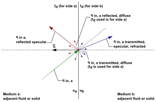
Incident radiant energy that is transmitted through a semi-transparent wall can be transmitted
specularly and diffusely. Radiation can also be reflected at the interior wall back to the
surrounding medium if the refractive index  for the fluid zone that represents medium
  is different than the refractive index
  for medium
  . Reflected radiation can be reflected specularly and diffusely. The fraction
of diffuse versus specular radiation that is transmitted and reflected depends on the diffuse
fraction for the wall. The special cases of purely diffuse and purely specular transmission
and reflection on semi-transparent walls is presented in the following sections.
. Reflected radiation can be reflected specularly and diffusely. The fraction
of diffuse versus specular radiation that is transmitted and reflected depends on the diffuse
fraction for the wall. The special cases of purely diffuse and purely specular transmission
and reflection on semi-transparent walls is presented in the following sections.
Note: For the case of a zero-thickness wall, the wall material's refractive index has no effect on refraction/reflection and only the refractive indices of the adjoining mediums are considered.
If the semi-transparent wall has thickness, then the thickness
and the absorption coefficient determine the absorptivity of the ‘thin’
wall. If either the wall thickness or absorption coefficient is set
to  , then the wall has no absorptivity. Although incident
radiation can be absorbed in a semi-transparent wall that has thickness,
the default is that the absorbed radiation flux does not affect the
energy equation, which can result in an energy imbalance and possibly
an unexpected temperature field. The exception is when shell conduction
is used (available in 3D only). With shell conduction there is full
correspondence between energy and radiation. If the wall is expected
to have significant absorption/emission, then it may be better to
model the thickness explicitly with solid cells, where practical. Ansys Fluent does
not include emission from the surface of semi-transparent walls (due
to defined internal emissivity), except when a temperature boundary
condition is defined.
, then the wall has no absorptivity. Although incident
radiation can be absorbed in a semi-transparent wall that has thickness,
the default is that the absorbed radiation flux does not affect the
energy equation, which can result in an energy imbalance and possibly
an unexpected temperature field. The exception is when shell conduction
is used (available in 3D only). With shell conduction there is full
correspondence between energy and radiation. If the wall is expected
to have significant absorption/emission, then it may be better to
model the thickness explicitly with solid cells, where practical. Ansys Fluent does
not include emission from the surface of semi-transparent walls (due
to defined internal emissivity), except when a temperature boundary
condition is defined.
Consider the special case for a semi-transparent wall, when
the diffuse fraction  is equal to
  and all of the transmitted
and reflected radiant energy at the semi-transparent wall is purely
specular.
and all of the transmitted
and reflected radiant energy at the semi-transparent wall is purely
specular.
Figure 5.10: Reflection and Refraction of Radiation at the Interface Between
Two Semi-Transparent Media shows
a ray traveling from a semi-transparent medium  with refractive index
  to a semi-transparent
medium
to a semi-transparent
medium  with a refractive index
  in the direction
  . Surface
  of the interface is the side that faces medium
  ; similarly, surface
  faces medium
  . The interface normal
  is assumed to point into side
  . We distinguish between the intensity
  , the intensity in the direction
  on side
  of the interface, and the corresponding quantity
on the side
of the interface, and the corresponding quantity
on the side  ,
,  .
.
Figure 5.10: Reflection and Refraction of Radiation at the Interface Between Two Semi-Transparent Media
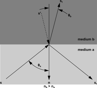
A part of the energy incident on the interface is reflected, and the rest is transmitted. The reflection is specular, so that the direction of reflected radiation is given by
 | (5–82) |
The radiation transmitted from medium  to medium
  undergoes refraction. The direction
of the transmitted energy,
undergoes refraction. The direction
of the transmitted energy,  , is given
by Snell’s law:
, is given
by Snell’s law:
 | (5–83) |
where  is the angle of incidence
and
is the angle of incidence
and  is the angle of transmission,
as shown in Figure 5.10: Reflection and Refraction of Radiation at the Interface Between
Two Semi-Transparent Media.
We also define the direction
is the angle of transmission,
as shown in Figure 5.10: Reflection and Refraction of Radiation at the Interface Between
Two Semi-Transparent Media.
We also define the direction
 | (5–84) |
The interface reflectivity on side  [447]
[447]
 | (5–85) |
represents the fraction of incident energy transferred from  to
to  .
.
The boundary intensity  in the
outgoing direction
in the
outgoing direction  on side
  of the interface is determined
from the reflected component of the incoming radiation and the transmission
from side
of the interface is determined
from the reflected component of the incoming radiation and the transmission
from side  . Thus
 | (5–86) |
where  is the
transmissivity of side
is the
transmissivity of side  in direction
  . Similarly,
the outgoing intensity in the direction
. Similarly,
the outgoing intensity in the direction  on side
  of the interface,
  , is given
by
, is given
by
 | (5–87) |
For the case  , the energy
transmitted from medium
, the energy
transmitted from medium  to medium
  in the incoming solid angle
  must be refracted
into a cone of apex angle
must be refracted
into a cone of apex angle  (see Figure 5.11: Critical Angle θc) where
 | (5–88) |
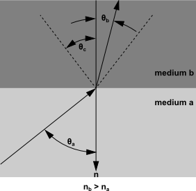
Similarly, the transmitted component of the radiant energy going
from medium  to medium
  in the cone of apex angle
  is refracted
into the outgoing solid angle
is refracted
into the outgoing solid angle  . For incident angles greater
than
. For incident angles greater
than  , total internal reflection
occurs and all the incoming energy is reflected specularly back into
medium
, total internal reflection
occurs and all the incoming energy is reflected specularly back into
medium  . The equations presented above can be applied to
the general case of interior semi-transparent walls that is shown
in Figure 5.9: DO Radiation on Interior Semi-Transparent Wall.
. The equations presented above can be applied to
the general case of interior semi-transparent walls that is shown
in Figure 5.9: DO Radiation on Interior Semi-Transparent Wall.
When medium  is external to the domain as in the case of an external
semi-transparent wall (Figure 5.12: DO Irradiation on External Semi-Transparent Wall),
is external to the domain as in the case of an external
semi-transparent wall (Figure 5.12: DO Irradiation on External Semi-Transparent Wall),  is given in Equation 5–86 as a part of the boundary condition inputs. You supply this incoming
irradiation flux in terms of its magnitude, beam direction, and the
solid angle over which the radiative flux is to be applied. Note that
the refractive index of the external medium is assumed to be
is given in Equation 5–86 as a part of the boundary condition inputs. You supply this incoming
irradiation flux in terms of its magnitude, beam direction, and the
solid angle over which the radiative flux is to be applied. Note that
the refractive index of the external medium is assumed to be  .
.
Consider the special case for a semi-transparent wall, when
the diffuse fraction  is equal to
  and all of the transmitted
and reflected radiant energy at the semi-transparent wall is purely
diffuse.
and all of the transmitted
and reflected radiant energy at the semi-transparent wall is purely
diffuse.
In many engineering problems, the semi-transparent interface
may be a diffuse reflector. For such a case, the interfacial reflectivity  is assumed independent of
  , and equal to
the hemispherically averaged value
, and equal to
the hemispherically averaged value  . For
. For  ,
,  and
and  are given by [597]
 | (5–89) |
 | (5–90) |
The boundary intensity for all outgoing directions on side  of the interface is given
by
of the interface is given
by
 | (5–91) |
Similarly for side  ,
,
 | (5–92) |
where
 | (5–93) |
 | (5–94) |
When medium  is external to the domain as in the case of an external
semi-transparent wall (Figure 5.12: DO Irradiation on External Semi-Transparent Wall),
is external to the domain as in the case of an external
semi-transparent wall (Figure 5.12: DO Irradiation on External Semi-Transparent Wall),  is given as
a part of the boundary condition inputs. You supply this incoming
irradiation flux in terms of its magnitude, beam direction, and the
solid angle over which the radiative flux is to be applied. Note that
the refractive index of the external medium is assumed to be
is given as
a part of the boundary condition inputs. You supply this incoming
irradiation flux in terms of its magnitude, beam direction, and the
solid angle over which the radiative flux is to be applied. Note that
the refractive index of the external medium is assumed to be  .
.
When the diffuse fraction  that you enter for a semi-transparent
wall is between
that you enter for a semi-transparent
wall is between  and
and  , the wall is partially diffuse and partially specular.
In this case, Ansys Fluent includes the reflective and transmitted
radiative flux contributions from both diffuse and specular components
to the defining equations.
, the wall is partially diffuse and partially specular.
In this case, Ansys Fluent includes the reflective and transmitted
radiative flux contributions from both diffuse and specular components
to the defining equations.
Figure 5.12: DO Irradiation on External Semi-Transparent Wall shows the general
case of an irradiation beam  applied to an exterior semi-transparent
wall with zero-thickness and a nonzero absorption coefficient for
the material property. Refer to the previous section for the radiation
effects of wall thickness on semi-transparent walls.
applied to an exterior semi-transparent
wall with zero-thickness and a nonzero absorption coefficient for
the material property. Refer to the previous section for the radiation
effects of wall thickness on semi-transparent walls.
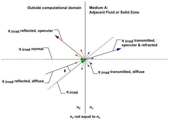
An irradiation flux passes through the semi-transparent wall
from outside the computational domain (Figure 5.12: DO Irradiation on External Semi-Transparent Wall) into the adjacent fluid or
solid medium a. The transmitted radiation
can be refracted (bent) and dispersed specularly and diffusely, depending
on the refractive index and the diffuse fraction that you provide
as a boundary condition input. Note that there is a reflected component
of  when the refractive index of the wall (
 ) is not equal
to
) is not equal
to  , as shown.
There is an additional flux beyond  that is applied when the Mixed or Radiation wall boundary
conditions are selected in the Thermal tab. This
external flux at the semi-transparent wall is computed by Ansys Fluent as
that is applied when the Mixed or Radiation wall boundary
conditions are selected in the Thermal tab. This
external flux at the semi-transparent wall is computed by Ansys Fluent as
 | (5–95) |
The fraction of the above energy that will enter into the domain depends on the transmissivity of the semi-transparent wall under consideration. Note that this energy is distributed across the solid angles (that is, similar treatment as diffuse component.)
Incident radiation can also occur on external semi-transparent walls. Refer to the previous discussion on interior walls for details, since the radiation effects are the same.
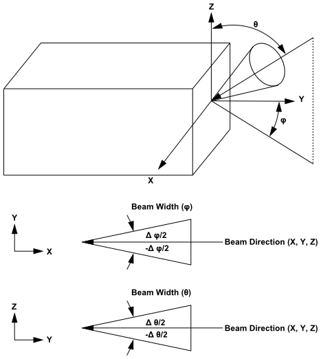
The irradiation beam is defined by the magnitude, beam direction, and beam width that you
supply. The irradiation magnitude is specified in terms of an incident radiant heat flux
( ). Beam width is specified as the solid angle over which the irradiation is
distributed (that is, the beam
). Beam width is specified as the solid angle over which the irradiation is
distributed (that is, the beam  and
and  extents). The default beam width in Ansys Fluent is
  degrees which is suitable for collimated beam radiation. Beam direction is
defined by the vector of the centroid of the solid angle. If you select the feature
Apply Direct Irradiation Parallel to the Beam in the
Wall boundary condition dialog box, then you supply
degrees which is suitable for collimated beam radiation. Beam direction is
defined by the vector of the centroid of the solid angle. If you select the feature
Apply Direct Irradiation Parallel to the Beam in the
Wall boundary condition dialog box, then you supply  for irradiation (Figure 5.12: DO Irradiation on External Semi-Transparent Wall) and
Ansys Fluent computes and uses the surface normal flux
for irradiation (Figure 5.12: DO Irradiation on External Semi-Transparent Wall) and
Ansys Fluent computes and uses the surface normal flux  in its radiation calculation. If this feature is not checked, then Fluent
automatically applies the source you specify, normal to the boundary such that = .
in its radiation calculation. If this feature is not checked, then Fluent
automatically applies the source you specify, normal to the boundary such that = .
Figure 5.13: Beam Width and Direction for External Irradiation Beam shows a schematic of the beam direction and beam width for the irradiation beam. You provide these inputs (in addition to irradiation magnitude) as part of the boundary conditions for a semi-transparent wall.
The irradiation beam can be refracted in medium a depending on the refractive index that is specified
for the particular fluid or solid zone material.
Where shell conduction is not active, there is only limited support for absorbing and emitting semi-transparent thin walls. In cases with significant emission or absorption of radiation in a participating solid material, such as the absorption of long wavelength radiation in a glass window, the use of semi-transparent thin walls can result in the prediction of unphysical temperatures in the numerical solution. In a 3-dimensional model this can be overcome by activating the shell conduction option for the respective thin wall. Otherwise, where possible, it is advisable to represent the solid wall thickness explicitly with one or more layers of cells across the wall thickness.
The discrete ordinates radiation model allows you to model a solid zone that has adjacent fluid or solid zones on either side as a "semi-transparent" medium. This is done by designating the solid zone to participate in radiation as part of the boundary condition setup. Modeling a solid zone as a semi-transparent medium allows you to obtain a detailed temperature distribution inside the semi-transparent zone since Ansys Fluent solves the energy equation on a per-cell basis for the solid and provides you with the thermal results. By default, however, the DO equations are solved in fluid zones, but not in any solid zones. Therefore, you will need to specify the solid zone as participating in radiation in the Solid dialog box as part of the boundary condition setup.
At specular walls and symmetry boundaries, the direction of
the reflected ray  corresponding
to the incoming direction
corresponding
to the incoming direction  is given by Equation 5–82. Furthermore,
 | (5–96) |
When rotationally periodic boundaries are used, it is important
to use pixelation in order to ensure that radiant energy is correctly
transferred between the periodic and shadow faces. A pixelation between  and
and  is recommended.
For opaque flow inlet and outlets, the treatment is described in Boundary Condition Treatment for the DTRM at Flow Inlets and outlets.
For transparent flow inlet and outlets, the boundary behaves similarly to an external semi-transparent wall, however, the irradiation flux passes through the transparent flow boundary from outside the computational domain into the adjacent fluid zone without getting reflected, absorbed or refracted. For details, see Semi-Transparent Exterior Walls.