


The population balance model is available with the mixture and Eulerian multiphase models.
This chapter provides basic instructions to set up and solve population balance problems in Ansys Fluent. This chapter describes the following:
This section describes the appropriate inputs for setting the population balance model. Using the double-precision version of Ansys Fluent when solving population balance problems is highly recommended.
Important: Note the following limitation of the population balance model: The model can be used only on one secondary phase, even if your problem includes additional secondary phases. A three-phase gas-liquid-solid case can be modeled, where the population balance model is used for the gas phase and the solid phase acts as a catalyst. However, if you are using the Inhomogeneous Discrete, more than one secondary phase can be used. The properties of the secondary phases selected for that method should be the same for consistency.
For more information, see the following sections:
- 26.6.1.1. Enabling the Population Balance Model
- 26.6.1.2. Defining Population Balance Boundary Conditions
- 26.6.1.3. Defining Population Balance Cell Zones Conditions
- 26.6.1.4. Specifying Population Balance Solution Controls
- 26.6.1.5. Coupling With Fluid Dynamics
- 26.6.1.6. Specifying Interphase Mass Transfer Due to Nucleation and Growth
- 26.6.1.7. Size Calculator
The below procedure for setting up a population balance problem includes only those steps necessary for the population balance model itself. You will need to set up other models, boundary conditions, and so on, as usual. See the Ansys Fluent User's Guide for details.)
Start the double-precision version of Ansys Fluent.
Enable either the mixture or Eulerian multiphase model.
In the Multiphase Model dialog box, open the Population Balance Model tab (Figure 26.91: The Multiphase Model Dialog Box - Population Balance Model Tab).
 Setup → Models
→ Population Balance
Setup → Models
→ Population Balance  Edit...
Specify the population balance method under Method.
If you select Discrete, you will need to specify the following parameters:
- Kv
specifies the value for the particle volume coefficient
 (as described in Particle Growth). By default, this coefficient
has a value of
(as described in Particle Growth). By default, this coefficient
has a value of  .
.- Definition
can be specified as a Geometric Ratio or as a File. If Geometric Ratio is selected, then the Ratio Exponent must be specified. If File is selected, you will click the Load File... button and select the bin size file that you want loaded.
You can input the diameter through the text file, with each diameter listed on a separate line, starting from the smallest to the largest diameter (one entry per line). Hence, you are not limited by the choices specified in the dialog box.
- Bins
specifies the number of particle size bins used in the calculation. The maximum number of bins allowed is 50.
- Ratio Exponent
specifies the exponent
 used in the discretization of the growth term volume
coordinate (see Numerical Method).
used in the discretization of the growth term volume
coordinate (see Numerical Method).- Min Diameter
specifies the minimum bin size
 .
.- Max Diameter
displays the maximum bin size, which is calculated internally.
To display a list of the bin sizes in the console window, click Print Bins. The bin sizes will be listed in order of size, from the largest to the smallest. This option is only available when the Geometric Ratio Definition is selected.
If you select Inhomogeneous Discrete under Method, you will specify the same parameters as for the Discrete model. Additionally, you can include more than one secondary phase in the bin definition. Enter the total number of Active Secondary Phases in your simulation.
Note: While reading bins through the Load File... option for the Inhomogeneous Discrete model, the corresponding phase name must be included, for example
(("air-1" (0.1 0.2
                      0.3)))
If you select Standard Moment under Method, you will specify the number of Moments under Parameters.
If you selected Quadrature Moment under Method, you will set the number of moments to either
4,6or8under Parameters.If you selected DQMOM under Method, you will select the DQMOM Phases from the list. You will also specify the following Parameters:
- Max Size
specifies the maximum size of the particle.
- Min Size
specifies the minimum size of the particle.
- Reference Length
is the reference particle size. Normally, the averaged size of the particle group should be sufficient.
- Min VOF
is the minimum VOF, where the total volume fraction of the particle phases (participating in DQMOM computations) is below the minimum value; the source terms caused by the breakage and coalescence are not computed in that cell for the DQMOM and VOF equations.
- Max VOF Change/Time Step
is the maximum VOF change in percentage for each DQMOM phase per time step, in order to smooth the convergence progress.
- Generate DQMOM Values
enables you to generate DQMOM values from PDF, CDF, or Overall Moments files. Each of the file formats and the way to generate the values are discussed in Generated DQMOM Values.
Note: The DQMOM method is restricted to a four-phase system, of which three secondary phases are directly involved in the DQMOM computation. Unsteady simulations are required to model breakage and coalescence and a well defined initial field is recommended, in which the abscissas are distinct. Only growth, breakage, and aggregation are the available phenomena. No nucleation is considered.
You can use the built-in size calculator to evaluate bubble sizes and/or droplet size limits. You can open the Size Calculator dialog box by clicking the Size Calculator... button and obtain the recommendations as described in Size Calculator. The tool provides estimated values based on best practices and engineering recommendations.
Select the secondary phase from the Phase drop-down list for which you want to apply the population balance model parameters.
For all population balance methods, you can enable the following under Phenomena :
- Nucleation Rate
enables you to specify the nucleation rate (
 ). You can select constant or
user-defined from the drop-down list. If you select
constant, specify a value in the adjacent field. If you
have a user-defined function (UDF) that you want to use to model the nucleation
rate, you can choose the user-defined option and specify
the appropriate UDF.
). You can select constant or
user-defined from the drop-down list. If you select
constant, specify a value in the adjacent field. If you
have a user-defined function (UDF) that you want to use to model the nucleation
rate, you can choose the user-defined option and specify
the appropriate UDF.Note: This option is not available when using the Inhomogeneous Discrete method.
- Growth Rate
enables you to specify the particle growth rate (m/s). You can select constant or user-defined from the drop-down list. If you select constant, specify a value in the adjacent field. If you have a user-defined function (UDF) that you want to use to model the growth rate, you can choose the user-defined option and specify the appropriate UDF.
Note: This option is not available when using the Inhomogeneous Discrete method.
- Aggregation Kernel
enables you to specify the aggregation kernel (
 ) and specify the Aggregation Factor.
 The Aggregation Factor (
 in Equation 14–737 in the Fluent Theory Guide) is used for the calibration of the aggregation
kernel.
in Equation 14–737 in the Fluent Theory Guide) is used for the calibration of the aggregation
kernel.For Rate, you can select constant, liao-aggregation-model, luo-model, free-molecular-model, turbulent-model, prince-blanch-model, or user-defined from the drop-down list:
If you select constant, specify a value in the adjacent field.
If you select liao-aggregation-model, the Liao Aggregation Model Parameters dialog box will open automatically. Note that because this is a modal dialog box, you must tend to it immediately.
You can specify the following parameters:
Surface Tension
Packing Limit: Is the maximum packing limit,
 in Equation 14–764 in the Fluent Theory Guide.
Coalescence Efficiency Coefficient:
 in Equation 14–771 in the Fluent Theory Guide.
Hamaker Constant:
 in Equation 14–776 in the Fluent Theory Guide.
Initial Film Thickness
Final Film Thickness
Buoyancy Coalescence Coefficient: Is
 in Equation 14–771 in the Fluent Theory Guide.
Turbulence Coalescence Coefficient: Is
 in Equation 14–770 in the Fluent Theory Guide.
Eddy Coalescence Coefficient: Is
 in Equation 14–778 in the Fluent Theory Guide.
Shear Coalescence Coefficient: Is
 in Equation 14–777 in the Fluent Theory Guide.
Wake Coalescence Coefficient: Is
 in Equation 14–780 in the Fluent Theory Guide.
For more information about this model and its parameters, see Liao Aggregation Kernel in the Fluent Theory Guide.
If you select luo-model, the Surface Tension for Population Balance dialog box will open automatically to enable you to specify the surface tension (see Figure 26.93: The Surface Tension for Population Balance Dialog Box). The aggregation rate for the model will then be calculated based on Luo’s aggregation kernel (as described in Particle Birth and Death Due to Breakage and Aggregation).
If you select free-molecular-model, then Equation 14–746 is applied.
If you select turbulent-model, the Hamaker Constant for Population Balance dialog box will open automatically to enable you to specify the Hamaker constant (see Figure 26.94: The Hamaker Constant for Population Balance Dialog Box). More information about this model is available in Turbulent Aggregation Kernel.
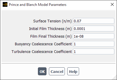
If you select prince-blanch-model, the Prince and Blanch Model Parameters dialog box will open automatically. Note that because this is a modal dialog box, you must tend to it immediately.
You can specify the following parameters:
Surface Tension
Initial Film Thickness: Is
 in Equation 14–756 in the Fluent Theory Guide.
Final Film Thickness: Is
 in Equation 14–756 in the Fluent Theory Guide.
Buoyancy Coalescence Coefficient: Is
 in Equation 14–762 in the Fluent Theory Guide.
Turbulence Coalescence Coefficient: Is
 in Equation 14–759 in the Fluent Theory Guide.
More information about this model is available in Prince and Blanch Aggregation Kernel.
If you have a user-defined function (UDF) that you want to use to model the aggregation rate, you can choose the user-defined option and specify the appropriate UDF.
- Breakage Kernel
enables you to specify the particle breakage rate (
 ) and the Breakage Factor.
 The Breakage Factor (
 in Equation 14–704 in the Fluent Theory Guide) is used for the calibration of the breakage
kernel.
in Equation 14–704 in the Fluent Theory Guide) is used for the calibration of the breakage
kernel.For Frequency, you can select constant, liao-breakage-model, luo-model, lehr-model, ghadiri-model, laakkonen-model, martinez-bazan-model, or user-defined from the Frequency drop-down list:
If you select constant, specify a value in the adjacent field.
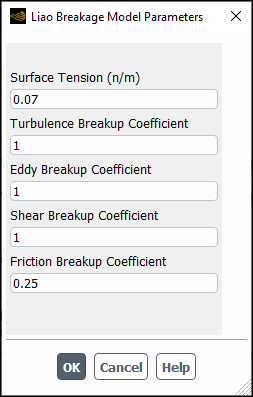
If you select liao-breakage-model, the Liao Breakage Model Parameters dialog box will open automatically. Note that because this is a modal dialog box, you must tend to it immediately.
You can specify the following parameters:
Surface Tension
Turbulence Breakup Coefficient: Is
 in Equation 14–720 in the Fluent Theory Guide.
Eddy Breakup Coefficient: Is
 in Equation 14–722 in the Fluent Theory Guide.
Shear Breakup Coefficient: Is
 in Equation 14–721 in the Fluent Theory Guide.
Friction Breakup Coefficient: Is
 in Equation 14–723 in the Fluent Theory Guide.
For more information about this model and its parameters, see Liao Breakage Kernel in the Fluent Theory Guide.
If you select luo-model, the Surface Tension for Population Balance dialog box will open automatically to enable you to specify the surface tension (see Figure 26.93: The Surface Tension for Population Balance Dialog Box). The frequency used in the breakage rate will then be calculated based on Luo’s breakage kernel (as described in Particle Birth and Death Due to Breakage and Aggregation).
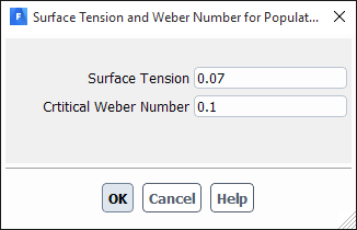
If you select lehr-model, the Surface Tension and Weber Number dialog box will open automatically to enable you to specify the surface tension and critical Weber number (see Figure 26.97: The Surface Tension and Weber Number Dialog Box). The frequency used in the breakage rate will then be calculated based on Lehr’s breakage kernel (as described in Particle Birth and Death Due to Breakage and Aggregation).
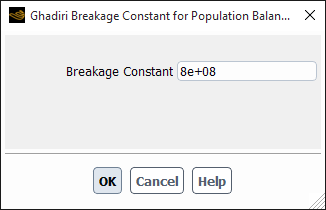
If you select ghadiri-model, the Ghadiri Breakage Constant for Population Balance dialog box will open automatically to enable you to specify the breakage constant (see Figure 26.98: The Ghadiri Breakage Constant for Population Balance Dialog Box). The frequency will then be calculated based on Ghadiri’s breakage kernel (as described in Particle Birth and Death Due to Breakage and Aggregation).
If you select laakkonen-model, the Surface Tension for Population Balance dialog box will open automatically to enable you to specify the Surface Tension and the constant C2 (Laakkonen Breakage Kernels). The frequency will then be calculated based on Laakkonen's breakage kernel (as described in Laakkonen Breakage Kernels).
When you select martinez-bazan-model, the Martinez-Bazan model is used to model the breakage rate. The Martinez-Bazan frequency predicts the breakage frequency of parent bubbles/particles based on the local values of a maximum stable bubble size as described in Martinez-Bazan Breakage Kernel in the Fluent Theory Guide. This model is widely used in stirred tank reactors.
If you have a user-defined function (UDF) that you want to use to model the frequency for the breakage rate, you can choose the user-defined option and specify the appropriate UDF.
If you selected constant, ghadiri-model, laakkonen-model, martinez-bazan-model, or user-defined for Frequency, then you can specify the probability density function used to calculate the breakage rate by making a selection in the PDF drop-down list. You can select the following models for the breakage PDF:
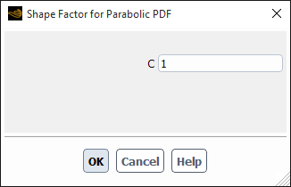
If you select parabolic, the Shape Factor for Parabolic PDF dialog box will open automatically to enable you to specify the shape factor C (see Figure 26.99: The Shape Factor for Parabolic PDF Dialog Box). The PDF used in the breakage rate will then be calculated according to Equation 14–724 (as described in Particle Birth and Death Due to Breakage and Aggregation).
When you select laakkonen, the daughter PDF is modeled using the Laakkonen model as described in Laakkonen Breakage Kernels in the Fluent Theory Guide.
If you select generalized, the Generalized pdf for multiple breakage dialog box will open automatically (Figure 26.100: The Generalized pdf for multiple breakage Dialog Box).
Perform the following steps in the Generalized pdf for multiple breakage dialog box:
Select either One Term or Two Term from the Options list. Your selection will determine whether
 in Equation 14–730 is 0 or 1,
respectively.
in Equation 14–730 is 0 or 1,
respectively.Enter a value for the averaged Number of Daughters. It can be any real number (including non-integers, such as 2.5), as long as it is not less than 2.
Define the parameter(s) for Equation 14–730 in the Input Parameters group box. When One Term is selected from the Options list, you must enter a value for qi0. When Two Term is selected from the Options list, you must enter values for wi0, pi0, qi0, ri0, and qi1. For information about appropriate values for these parameters to result in the daughter distributions shown in Table 14.6: Daughter Distributions, see Table 14.7: Daughter Distributions (cont.).
Note: For the equal-size generalized pdf breakage distribution, the value for qi0 should be set to
1e20.Click the Validate/Apply button to save the settings. The text boxes in the All Parameters group box will be updated, using the values you entered in the Input Parameters group box, as well as values derived from the constraints shown in Equation 14–731 – Equation 14–733.
Verify that the values in the All Parameters group box represent your intended PDF before clicking Close.
When you select inverted-u-pdf, the inverted distribution PDF is used to model bubble breakage as described in Inverted U-PDF in the Fluent Theory Guide. This model can produce more physical results in simulations of certain impeller-agitated mixing tanks.
If you have a user-defined function (UDF) that you want to use to model the PDF for the breakage rate, you can choose the user-defined option and specify the appropriate UDF. See UDFs for Population Balance Modeling for details about UDFs for the population balance model.
Choose between the default Hagesather formulation and the Ramakrishna formulation. Detailed information about these two methods can be found in Breakage Formulations for the Discrete Method.
Note: Since most standard breakage/aggregation kernels depend on the primary phase turbulence, Ansys Fluent assumes a volume fraction cutoff of 0.8 or less of secondary phases (that is, 0.2 or more of a primary phase) for breakage or aggregation to be enabled. This cutoff volume fraction can be modified by the following text command:
define/models/multiphase/population-balance/phenomena/breakage-aggregation-vof-cutoff(Discrete, QMOM, and Inhomogeneous Discrete models only) If you want to account for bubble expansion due to large changes in hydrostatic pressure in compressible flows, enable Include Expansion. The bubble expansion is modeled as a growth term in the Population Balance equations (Equation 14–703). This can be relevant in applications such as deep-water drilling. For more information, see Particle Growth.
Note: The secondary phase must be modeled as compressible. This option is currently available for Discrete and QMOM only.
Specify the boundary conditions for the solution variables.
Setup →  Boundary Conditions
Specify the initial guess for the solution variables.
Solution →
Initialization
Solve the problem and perform relevant postprocessing functions.
Solution →
Run Calculation
See Postprocessing for the Population Balance Model for details about postprocessing.
When using the DQMOM model, you have the option of generating DQMOM values from three different file formats. To do so, select Overall Moments, PDF or CDF under Generate DQMOM Values and then click the Load File… button. The Select File dialog box will open where you will select the appropriate file. Clicking in the Select File dialog box will result in the file being read and calculations carried out. The DQMOM values will be printed in the console.
DQMOM Values Produced From PDF, CDF Files, or Overall Moments for the Particles —
Three quadrature points are assumed, namely QP0, QP1, and QP2 (see Figure 26.102: DQMOM Values Produced From a PDF File).
Length,Volume Fraction, andDQMOM-m4values are given. The latter two can be used for initial fields of VOF and DQMOM as well as boundary conditions.For verification purposes, the first six moments are also given together with the total volume fraction of all particles from the PDF or CDF file. It is your responsibility to make sure that these values are correct, especially the total volume fraction.
The definition of the first six moments of the particles is length based for the overall moments, described in The Quadrature Method of Moments (QMOM).
In PDF or CDF format, the resultant volume fraction is normally given as unity. If you want the real particle volume fraction to be reflected in the mixture, the second column of the PDF or CDF data file need to be multiplied by the value of the real volume fraction. Another way is to multiply the values of the generated DQMOM volume fraction and DQMOM-m4 using the real particle volume fraction.
PDF File Format —
The probability density function (PDF) is defined by the probability distribution of particles in terms of the volume fraction over the particle length (namely the diameter of the particle).
The integration of PDF over all possible particle length (normally from 0 to the maximum diameter) shall give a value of unity or the real value of the volume fraction of all participating particles.
The following file format is required (as shown below):
An integer number specified in the first line, indicating the number of data pairs to follow
The data in the 1st column specifying the length or diameter of particles in ascending order in meters (m)
The data in the 2nd column specifying the probability density function. Be aware that the integration of the PDF over the length shall result in a value of volume fraction for that particular particle length range
37
5e-6	0.000058e6
10e-6	0.000271e6
15e-6	0.000669e6
20e-6	0.001264e6
25e-6	0.002062e6
30e-6	0.003055e6
35e-6	0.004228e6
40e-6	0.005549e6
45e-6	0.006972e6
50e-6	0.008439e6
55e-6	0.00988e6
60e-6	0.011217e6
65e-6	0.012366e6
70e-6	0.013253e6
75e-6	0.013811e6
80e-6	0.013996e6
85e-6	0.013789e6
90e-6	0.013199e6
95e-6	0.012268e6
100e-6	0.011062e6
105e-6	0.009668e6
110e-6	0.00818e6
115e-6	0.006694e6
120e-6	0.00529e6
125e-6	0.004033e6
130e-6	0.002962e6
135e-6	0.002093e6
140e-6	0.00142e6
145e-6	0.000925e6
150e-6	0.000576e6
155e-6	0.000344e6
160e-6	0.000196e6
170e-6	0.000055e6
180e-6	0.000012e6
190e-6	0.000002e6
200e-6	0.
210e-6  0.
CDF File Format —
The cumulative density function (CDF) is defined as the integration of PDF over all possible particles up to the length
 , resulting in a value of volume fraction for all particles
less than length
, resulting in a value of volume fraction for all particles
less than length  .
.The value of the CDF at the maximum particle length/diameter shall be unity, or the real value of the volume fraction of all particles in the mixture.
The following file format is required (as shown below):
An integer number specified in the first line, indicating the number of data pairs to follow
The data in the 1st column specifying the length or diameter of particles in ascending order in meters (m)
The data in the 2nd column specifying the cumulative density function in terms of the volume fraction of particles
 at the maximum particle length
37
5e-6	0
10e-6	0.109e-2
15e-6	0.16e-2
20e-6	0.175e-2
25e-6	0.208e-2
30e-6	0.304e-2
35e-6	0.614e-2
40e-6	1.5e-2
44e-6   3.e-2
45e-6   3.44e-2
50e-6	6.573e-2
55e-6	11.19e-2
60e-6	17.11e-2
65e-6	24.17e-2
70e-6	32.007e-2
75e-6	40.243e-2
80e-6	48.397e-2
85e-6	56.453e-2
90e-6	63.823e-2
95e-6	70.53e-2
100e-6	76.073e-2
105e-6	81e-2
110e-6	85.057e-2
115e-6	88.187e-2
120e-6	90.89e-2
125e-6	92.897e-2
130e-6	94.437e-2
135e-6	95.543e-2
140e-6	96.523e-2
145e-6	97.173e-2
150e-6	97.717e-2
155e-6	98.007e-2
160e-6	98.363e-2
170e-6	98.88e-2
180e-6	99.16e-2
190e-6	99.327e-2
200e-6	100.e-2
Overall Moments File Format —
The third option is to specify the first six moments for all particles as shown below.
The following file format is required (as shown below):
An integer number specified in the first line, indicating the number of data (moments) to follow. By default, this shall be 6
six moments from moment-0 to moment-5 are given in that order. The definition of the first six moments is based on length as described in The Quadrature Method of Moments (QMOM)
As a check for moments,
 . In the values given below, volume fraction is assumed
to be unity and
. In the values given below, volume fraction is assumed
to be unity and  is assumed to be
6
1.120556e+013
4.022475e+008
2.523370e+004
1.909857e+000
1.611191e-004
1.498663e-008
To define boundary conditions specific to the population balance model, use the following procedure:
In the Boundary Conditions task page, select the secondary phase(s) in the Phase drop-down list and then open the appropriate boundary condition dialog box (for example, Figure 26.103: Specifying Inlet Boundary Conditions for the Population Balance Model).
Setup →
Boundary Conditions
In the Multiphase tab, under Boundary Condition, select the type of boundary condition for each bin (for the discrete method) or moment (for SMM and QMOM) as either Specified Value or Specified Flux.
Note that the boundary condition variables (for example, Bin-0) are labeled according to the following:
bin/moment -
 th bin/moment
where the
 th
bin/moment can range from 0 (the first bin
or moment) to
th
bin/moment can range from 0 (the first bin
or moment) to  , where
  is the number of bins/moments that you entered in the
Population Balance Model tab.
is the number of bins/moments that you entered in the
Population Balance Model tab.Under Population Balance Boundary Value, enter a value or a flux as appropriate.
If you selected Specified Value for the selected boundary variable, enter a value in the field adjacent to the variable name. This value will correspond to the variable
 in Equation 14–786 (for the discrete method) or
  in Equation 14–801 (for SMM or QMOM). If you are using either of the discrete methods and have
selected Specified Value for all bins, you can optionally
specify a log-normal distribution and have Fluent automatically initialize the
bin fractions accordingly to a log-normal distribution (see Initializing Bin Fractions With a Log-Normal Distribution).
in Equation 14–801 (for SMM or QMOM). If you are using either of the discrete methods and have
selected Specified Value for all bins, you can optionally
specify a log-normal distribution and have Fluent automatically initialize the
bin fractions accordingly to a log-normal distribution (see Initializing Bin Fractions With a Log-Normal Distribution).If you selected Specified Flux for the selected boundary variable, enter a value in the field adjacent to the variable name. This value will be the spatial particle volume flux
 .
.
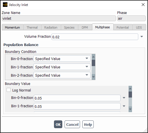
When using one of the discrete methods with Specified Value selected as the boundary condition for all bins, you can have Fluent populate the bin fractions according to a log-normal distribution characterized by a mean and standard deviation that you supply. For details of the log-normal distribution, refer to The Log-Normal Distribution.
Important: The log-normal initialization feature is only meaningful and should only be used when Specified Value is selected for all bins under Boundary Condition.
To use the log-normal distribution, perform the following steps.
Enable Log Normal in the Boundary Value group box.
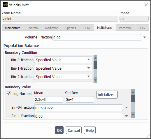
Enter values for the Mean and Std Dev of the desired distribution.
Click Initialize...
For the Discrete and Inhomogeneous Discrete population balance models, you can specify source terms for bin fractions. For general information about defining source terms, see Defining Mass, Momentum, Energy, and Other Sources. For additional details, see Procedure for Defining Sources and Discrete Bin Fraction Sources for the Population Balance Model.
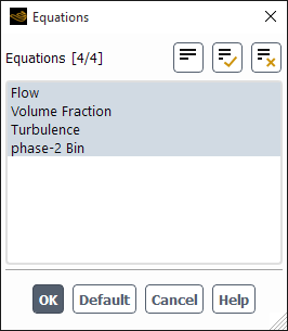
In the Equations dialog box (Figure 26.104: The Equations Dialog Box), equations for each bin (for example, phase-2 Bin) will appear in the Equations list.
![]() Solution → Controls
Solution → Controls
![]() Equations...
Equations...
The default value under Under-Relaxation Factors (in the
Solution Controls task page) for the population balance equations
is 0.5, and the default Discretization
scheme (in the Solution Methods task page) is First Order
Upwind.
To couple population balance modeling of the secondary phase(s) with the overall
problem fluid dynamics, a Sauter mean diameter ( in Equation 14–808) may
be used to represent the particle diameter of the secondary phase. The Sauter mean
diameter is defined as the ratio of the third moment to the second moment for the SMM and
QMOM. For the discrete method, it is defined as
in Equation 14–808) may
be used to represent the particle diameter of the secondary phase. The Sauter mean
diameter is defined as the ratio of the third moment to the second moment for the SMM and
QMOM. For the discrete method, it is defined as
 | (26–27) |
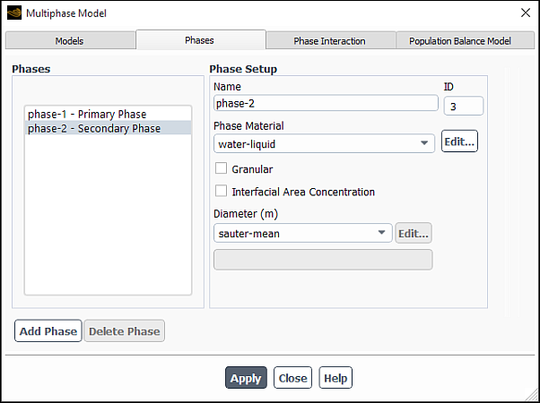
To specify the Sauter mean diameter as the secondary phase particle diameter, open the Phases tab
![]() Setup → Models
→ Multiphase
Setup → Models
→ Multiphase ![]() Edit...
Edit...
In the Multiphase Model dialog box (Phases tab) (for example, Figure 26.105: Setting the Secondary Phase for Hydrodynamic Coupling), select sauter-mean from the Diameter drop-down list under Properties. Note that a constant diameter or user-defined function may also be used.
In applications that involve the creation, dissolution, or growth of particles (such
as crystallization), the total volume fraction equation for the particulate phase will
have source terms due to these phenomena. The momentum equation for the particulate phase
will also have source terms due to the added mass. In Ansys Fluent, the mass source term can
be specified using the UDF hook DEFINE_HET_RXN_RATE, as described
in
DEFINE_HET_RXN_RATE Macro, or using the Phase
Interaction tab, described below.
As an example, in crystallization, particles are created by means of nucleation
( ), and a growth rate (
 ) can also be specified. The mass transfer rate of formation (in
 ) of particles of all sizes is then
 | (26–28) |
For the discrete method, the mass transfer rate due to growth can be written as
 | (26–29) |
If the nucleation rate is included in the total mass transfer, then the mass transfer becomes
 | (26–30) |
Important: For the discrete method, the sources to the population balance equations must sum to
the total mass transfer rate. To access the sources, you can use the macro
C_PB_DISCI_PS (cell, thread, i).
See UDFs for Population Balance Modeling for more information about macros for population balance variables.
For the SMM, only a size-independent growth rate is available. Hence, the mass transfer rate can be written as
 | (26–31) |
For the QMOM, the mass transfer rate can be written as
 | (26–32) |
For both the SMM and QMOM, mass transfer due to nucleation is negligible, and is not taken into account.
Important: Note that for crystallization, the primary phase has multiple components; at the very least, there is a solute and a solvent. To define the multicomponent multiphase system, you will need to activate Species Transport in the Species Model dialog box for the primary phase after activating the multiphase model. The rest of the procedure for setting up a species transport problem is identical to setting up species in single phase. The heterogeneous reaction is defined as:

When the population balance model is activated, mass transfer between phases for non-reacting species (such as boiling) and heterogeneous reactions (such as crystallization) can be done automatically, in lieu of hooking a UDF.
For simple unidirectional mass transfer between primary and secondary phases due to nucleation and growth phenomena of non-reacting species, configure the following settings:
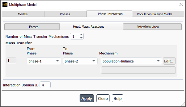
In the Multiphase Model dialog box, open the Phase Interaction > Heat, Mass, Reactions > Mass tab (Figure 26.106: The Phase Interaction Tab for Non-reacting Species).
Setup → Models
→ Multiphase
Edit...
Specify the Number of Mass Transfer Mechanisms involved in your case.
For each mechanism, specify the phase of the source material under From Phase and the phase of the destination material phase under To Phase.
From the Mechanism drop down list, select one of the mechanisms:
- none
if you do not want any mass transfer between the phases.
- constant-rate
for a fixed, user-specified rate.
- user-defined
if you hooked a UDF describing the mass transfer mechanism.
- population-balance
for an automated method of mass transfer, not involving a UDF. The nucleation and the growth rates calculated by the population balance kernels are used for mass transfer.
Note: For the Inhomogeneous Discrete population balance model, where there is more than one secondary phase, you can select
population-balanceas the mechanism of mass transfer between the solvent phase (say for crystallization) and each of the solute phases defined under the Inhomogeneous Discrete population balance model.Click to save the settings.
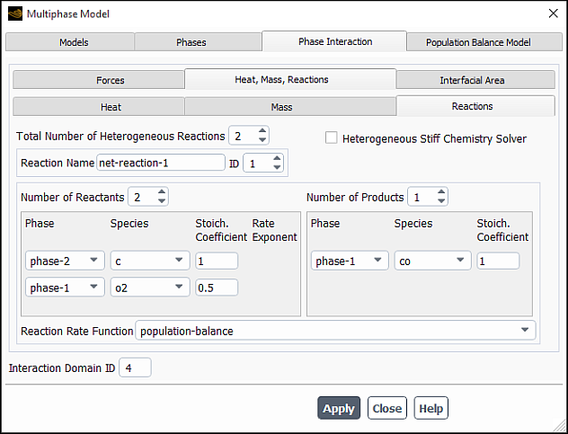
For heterogeneous reactions, configure the following settings:
For the primary phase, activate the Species Transport model.
Open the Phase Interaction > Heat, Mass, Reactions > Reactions tab in the Multiphase Model dialog box (Figure 26.107: The Reactions Tab for a Heterogeneous Reaction).
Setup → Models
→ Multiphase
Edit...
Under the Reactions tab, specify the stoichiometry for the reactant and the product.
Select
population-balanceas the Reaction Rate Function.Click to save the settings.
Either this method or the use of the UDF, described in
DEFINE_HET_RXN_RATE Macro, will produce the same results.
For the Inhomogeneous Discrete population balance model involving
nucleation and growth, you can select population-balance as the
Reaction Rate Function for each heterogeneous reaction you have set
up. To learn how to set up reactions, go to Specifying Heterogeneous Reactions in the User's Guide.
The size calculator provides estimation for appropriate bubble sizes and/or droplet size limits. To use this tool:
Click Size Calculator... in the Population Balance Model tab (Parameters group).
In the Size Calculator dialog box that opens, adjust the following parameters in the Fluid Properties group box:
Gravity
PB Phase Density
Primary Phase Density
Primary Phase Viscosity
Surface Tension Coefficient
Note the following:
When you open the dialog box for the first time, the entry fields in the Fluid Properties group box will be pre-populated with the case fluids information if constant properties are used. Otherwise, it will be pre-populated with gas-liquid information under standard pressure/temperature conditions. You need to review these values and modify them, as necessary.
Gravity refers to the gravity magnitude, which is computed based on the operating conditions specification.
Click Calculate.
In the Calculated Diameters group box, the solver gives the following fluid particle size estimations:
For bubbly flows:
Minimum Empirical Limit: This size is based on the minimum particle size limit for typical experimental acquisition methods.
Lift Sign Inversion: This size is calculated using the sign inversion from Equation 14–306 in the Fluent Theory Guide.
Maximum Stable Bubble – Eo = 10: This size is calculated using the modified Eötvös number calculated from Equation 14–308 in the Fluent Theory Guide.
Maximum Stable Bubble – Capillary Length: This size is calculated as 4 times the capillary length. It is based on the maximum diameter before a bubble disintegrates or starts breaking down as given by Ishii and Zuber ("Drag Coefficient and Relative Velocity in Bubbly, Droplet or Particulate Flows" in the Fluent Theory Guide). Typically, interfacial forces are empirically limited to this size.
For droplets flows:
Minimum Empirical Limit: Same as for bubbly flows.
Maximum Stable Droplet – We=12: This size is calculated using a Weber number of 12.0, and it represents the maximum diameter at which droplets start disintegrating.
Maximum Stable Droplet – Taylor Limit: This size is calculated using twice the capillary length, and it should be used if the stability of the droplet in the flow is governed by Taylor instabilities.
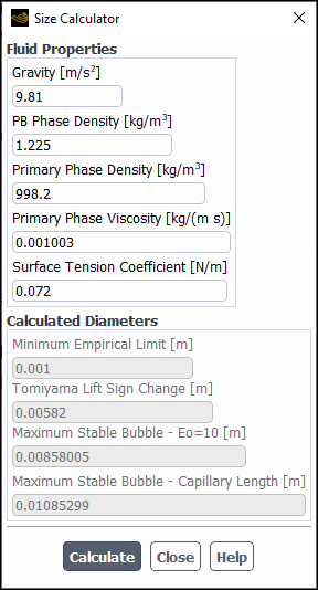
The recommended values will be also printed in the Fluent console.
You can use these recommendations as inputs to the Population Balance model.
In simulations that involve the QMOM population balance model, Ansys Fluent sometimes suppresses the calculation of sources in cells of very low volume fraction to avoid potential convergence problems. However, in certain cases this has been found to be counterproductive because the computation of sources in all cells can be beneficial for a robust solution. To invoke the calculation of all the sources regardless of the local volume fraction, you can use the following text command:
define/models/multiphase/population-balance/expert/qmom/retain-qmom-sources-for-low-vof?Retain QMOM sources? [no]yes
Ansys Fluent provides postprocessing options for displaying, plotting, and reporting various particle quantities, which include the main solution variables and other auxiliary quantities.
Solution variables that can be reported for the population balance model are:
Bin-i fraction (discrete method only), where i is N-1 bins/moments.
Number density of Bin-i fraction (discrete method only)
Diffusion Coef. of Bin-i fraction/Moment-i
Sources of Bin-i fraction/Moment-i
Moment-i (SMM and QMOM only)
Abscissa-i (QMOM method only)
Weight-i (QMOM method only)
Bin-i fraction ( ) is the total volume fraction for the
  th size bin when using the discrete method. Number
density of Bin-i fraction is the number density (
th size bin when using the discrete method. Number
density of Bin-i fraction is the number density ( ) in
) in  for the
  th size bin. Moment-i is the
 th moment of the distribution when using the standard method of
moments or the quadrature method of moments.
th moment of the distribution when using the standard method of
moments or the quadrature method of moments.
Important:
Though the diffusion coefficients of the population variables (for example, Diffusion Coef. of Bin-i fraction/Moment-i) are available, they are set to zero because the diffusion term is not present in the population balance equations.
In the Inhomogeneous Discrete population balance method involving 'n' bins, bin-0 and bin-(n-1) correspond to the largest and smallest bin sizes respectively.
The sources of bin
available for post-processing represent the total of sources due
to nucleation, growth, breakage, and coalescence phenomena and do not include any
source terms specified for bins in the cell zone condition dialog box (for example,
the Fluid dialog box).
Two options are available in the Results ribbon tab that allow you to report computed moments and number density on selected surfaces or cell zones of the domain.
You can compute moments for the population balance model using the Population Balance Moments dialog box (Figure 26.109: The Population Balance Moments Dialog Box).
![]() Results → Model Specific
→ Population Balance
→ Moments...
Results → Model Specific
→ Population Balance
→ Moments...
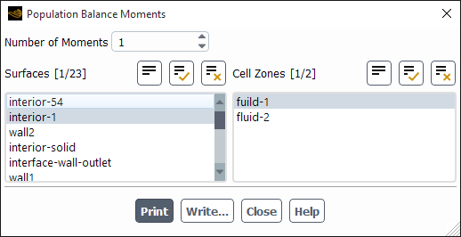
The steps for computing moments are as follows:
For the discrete method, specify the Number of Moments. For the SMM and QMOM, the number of moments is set equal to the number of moments that were solved, and therefore cannot be changed.
For a surface average, select the surface(s) on which to calculate the moments in the Surfaces list.
For a volume average, select the volume(s) in which to calculate the moments in the Cell Zones list.
Click to display the moment values in the console window.
To save the moment calculations to a file, click Write... and enter the appropriate information in the resulting Select File dialog box. The file extension should be .pb.
You can display the number density function for the population balance model using the Number Density Function dialog box (Figure 26.110: The Number Density Function Dialog Box).
![]() Results → Model Specific
→ Population Balance → Number
Density...
Results → Model Specific
→ Population Balance → Number
Density...
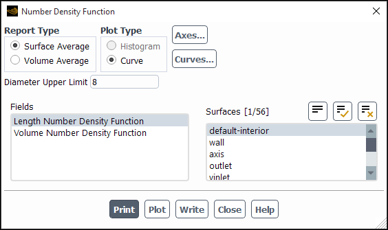
The steps for displaying the number density function are as follows:
Specify the Report Type as either a Surface Average or a Volume Average.
Under Plot Type, specify how you would like to display the number density function data.
- Histogram
displays a histogram of the discrete number density (
 ). The number of divisions in the histogram is equal to the
number of bins specified in the Population Balance Model
tab of the Multiphase Model dialog box. This option is
available only with the discrete method.
). The number of divisions in the histogram is equal to the
number of bins specified in the Population Balance Model
tab of the Multiphase Model dialog box. This option is
available only with the discrete method.- Curve
displays a smooth curve of the number density function.
(Quadrature Moment method only) Specify Diameter Upper Limit to reconstruct the length or volume-based number density function based on the moments predicted by QMOM (see Reconstructing the Particle Size Distribution from Moments in the Fluent Theory Guide for more information).
The moments are calculated by integrating the area under the number density curve. The accuracy of the calculations is dependent on the integration limit. Typically, this is expressed in terms of the mean of the distribution and is specified in the Diameter Upper Limit field. The default value of 1.5 means that the maximum diameter value considered is 1.5 times the mean of the distribution.
In the Fields list, select the data to be plotted.
- Discrete Number Density
(
 ) is the number of particles per unit volume of physical
space in the
) is the number of particles per unit volume of physical
space in the  th size bin plotted against particle diameter size
 . This option is available only with the discrete
method.
. This option is available only with the discrete
method.- Length Number Density Function
(
 ) is the number of particles per unit volume of physical
space per unit particle length plotted against particle diameter.
) is the number of particles per unit volume of physical
space per unit particle length plotted against particle diameter.- Volume Number Density Function
(
 ) is the number of particles per unit volume of physical
space per unit particle volume plotted against particle volume.
) is the number of particles per unit volume of physical
space per unit particle volume plotted against particle volume.
Choose the cell zones on which to plot the number density function data in the Cell Zones list.
Click Plot... to display the data.
(optional) Click Print to display the number density function data in the console window.
Click Write to save the number density function data to a file. The Select File dialog box will open, where you can specify a name and save a file containing the plot data. The file extension should be .pbd.
This section contains the following sections:
The macros listed in Table 26.14: Macros for Population Balance Variables Defined in sg_pb.h
can be used to return
real variables associated with the population balance model.
The variables are available in both the pressure-based and density-based solvers. The
macros are defined in the sg_pb.h header file, which is included
in udf.h.
Table 26.14: Macros for Population Balance Variables Defined in sg_pb.h
| Macro | Argument Types | Returns |
|---|---|---|
C_PB_DISCI
|
cell_t c, Thread *t, int i
| ( ) the total volume fraction for the ) the total volume fraction for the  th size bin
 |
C_PB_SMMI
|
cell_t c, Thread *t, int i
|
 th moment
 |
C_PB_QMOMI
|
cell_t c, Thread *t, int i
|
 th moment, where
|
C_PB_QMOMI_L
|
cell_t c, Thread *t, int i
| abscissa  , where , where 
|
C_PB_QMOMI_W
|
cell_t c, Thread *t, int i
| weight  , where , where 
|
C_PB_DISCI_PS
|
cell_t c, Thread *t, int i
| net source term to  th size bin
 |
C_PB_SMMI_PS
|
cell_t c, Thread *t, int i
| net source term to  th moment
 |
C_PB_QMOMI_PS
|
cell_t c, Thread *t, int i
| net source term to  th moment
 |
This section contains descriptions of DEFINE macros for the
population balance model. Definitions of each DEFINE macro are
contained in the udf.h header file.
You can use the DEFINE_PB_BREAK_UP_RATE_FREQ macro if you
want to define the breakage frequency using a UDF. The function is executed at the
beginning of every time step.
DEFINE_PB_BREAK_UP_RATE_FREQ(name, cell, thread, d_1)
| Argument Type | Description |
|---|---|
char name
| UDF name |
cell_t cell
| Cell index |
Thread *thread
| Pointer to the secondary phase thread associated with d_1 |
real d_1
| Parent particle diameter or length |
| Function returns | |
real
|
There are four arguments to DEFINE_PB_BREAK_UP_RATE_FREQ:
name, cell,
thread, and d_1. You will supply
name, the name of the UDF. cell,
thread, and d_1 are variables that
are passed by the Ansys Fluent solver to your UDF.
Included below is an example of a UDF that defines a breakage frequency (see Particle Birth and Death Due to Breakage and Aggregation) that is based on the work of Tavlarides [123], such that
 | (26–33) |
where  and
and  are constants with values of 0.00481 and 0.08, respectively,
 is the turbulence energy dissipation rate of the primary phase,
 is the parent diameter,
  is the surface tension,
  is the volume fraction of the dispersed phase, and
  is the density of the dispersed phase.
/************************************************************************
 UDF that computes the particle breakage frequency
 *************************************************************************/

 #include "udf.h"
 #include "sg_pb.h"
 #include "sg_mphase.h"

 DEFINE_PB_BREAK_UP_RATE_FREQ(break_up_freq_tav, cell, thread, d_1)
 {
     real epsi, alpha, f1, f2, rho_d;
     real C1 = 0.00481, C2 = 0.08, sigma = 0.07;
     Thread *tm = THREAD_SUPER_THREAD(thread);/*passed thread is phase*/
     epsi = C_D(cell, tm);
     alpha = C_VOF(cell, thread);
     rho_d = C_R(cell, thread);
     f1 = pow(epsi, 1./3.)/((1.+alpha)*pow(d_1, 2./3.));
     f2 = -(C2*sigma*(1.+alpha)*(1.+alpha))/(rho_d*pow(epsi,2./3.)*pow(d_1, 5./3.));
     return C1*f1*exp(f2);
 }
You can use the DEFINE_PB_BREAK_UP_RATE_PDF macro if you
want to define the breakage PDF using a UDF. The function is executed at the beginning
of every time step.
DEFINE_PB_BREAK_UP_RATE_PDF(name, cell, thread, d_1, thread_2,
                d_2)
| Argument Type | Description |
|---|---|
char name
| UDF name |
cell_t cell
| Cell index |
Thread *thread
| Pointer to the secondary phase thread associated with d_1 |
real d_1
| Parent particle diameter or length |
Thread *thread_2
| Pointer to the secondary phase thread associated with d_2 |
real d_2
| Diameter of one of the daughter particles after breakage; the second daughter particle diameter is calculated by conservation of particle volume |
| Function returns | |
real
|
There are six arguments to DEFINE_PB_BREAK_UP_RATE_PDF:
name, cell,
thread, d_1,
thread_2, and d_2. You will supply
name, the name of the UDF. cell,
thread, d_1,
thread_2, and d_2 are variables
that are passed by the Ansys Fluent solver to your UDF.
Note:
thread and thread_2 are the same
for the Discrete, QMOM and SMM models. They may be the same or different depending
on whether d_1 and d_2 belong to
the same phase or different phases for the Inhomogeneous model.
Included below is an example of a UDF that defines a breakage PDF (see Particle Birth and Death Due to Breakage and Aggregation) that is parabolic, as defined in Equation 14–724.
/************************************************************************
 UDF that computes the particle breakage PDF
 *************************************************************************/

 #include "udf.h"
 #include "sg_pb.h"
 #include "sg_mphase.h"

 DEFINE_PB_BREAK_UP_RATE_PDF(break_up_pdf_par, cell, thread, d_1, thread_2, d_2)
 {
     real pdf;
     real kv = M_PI/6.;

     real C = 1.0;

     real f_2, f_3, f_4;
     real V_prime = kv*pow(d_1,3.);
     real V = kv*pow(d_2,3.);

     f_2 = 24.*pow(V/V_prime,2.);
     f_3 = -24.*(V/V_prime);
     f_4 = 6.;

     pdf = (C/V_prime) + ((1.-C/2.)/V_prime)*(f_2 + f_3 + f_4);

     return 0.5*pdf;
 }
You can use the DEFINE_PB_COALESCENCE_RATE macro if you
want to define your own particle aggregation kernel. The function is executed at the
beginning of every time step.
DEFINE_PB_COALESCENCE_RATE(name, cell, thread, d_1, thread_2,
                d_2)
| Argument Type | Description |
|---|---|
char name
| UDF name |
cell_t cell
| Cell index |
Thread *thread
| Pointer to the secondary phase thread associated with d_1 |
Thread *thread_2
| Pointer to the secondary phase thread associated with d_2 |
real d_1, d_2
| Diameters of the two colliding particles |
| Function returns | |
real
|
There are six arguments to DEFINE_PB_COALESCENCE_RATE:
name, cell,
thread, d_1,
thread_2, and d_2. You will supply
name, the name of the UDF. cell,
thread, d_1, and
d_2 are variables that are passed by the Ansys Fluent solver to
your UDF. Your UDF will need to return the real value of the
aggregation rate.
Note:
thread and thread_2 are the same
for the Discrete, QMOM and SMM models. They may be the same or different depending
on whether d_1 and d_2 belong to
the same phase or different phases for the Inhomogeneous model.
Included below is an example UDF for a Brownian aggregation kernel. In this example, the aggregation rate is defined as

where 
 .
.
/************************************************************************
 UDF that computes the particle aggregation rate
 *************************************************************************/

 #include "udf.h"
 #include "sg_pb.h"
 #include "sg_mphase.h"

 DEFINE_PB_COALESCENCE_RATE(aggregation_kernel,cell,thread,d_1,thread_2,d_2)
 {
      real agg_kernel;
      real beta_0 = 1.0e-17 /* aggregation rate constant */
      agg_kernel = beta_0*pow((d_1+d_2),2.0)/(d_1*d_2);
      return agg_kernel;
 }
You can use the DEFINE_PB_NUCLEATION_RATE macro if you want
to define your own particle nucleation rate. The function is executed at the beginning
of every time step.
DEFINE_PB_NUCLEATION_RATE(name, cell, thread)
| Argument Type | Description |
|---|---|
char name
| UDF name |
cell_t cell
| Cell index |
Thread *thread
| Pointer to the secondary phase thread |
| Function returns | |
real
|
There are three arguments to DEFINE_PB_NUCLEATION_RATE:
name, cell, and
thread. You will supply name, the
name of the UDF. cell and thread are
variables that are passed by the Ansys Fluent solver to your UDF. Your UDF will need to
return the real value of the nucleation rate.
Potassium chloride can be crystallized from water by cooling. Its solubility decreases linearly with temperature. Assuming power-law kinetics for the nucleation rate,

where 
 and
and  .
.
/************************************************************************
 UDF that computes the particle nucleation rate
 *************************************************************************/

 #include "udf.h"
 #include "sg_pb.h"
 #include "sg_mphase.h"
 DEFINE_PB_NUCLEATION_RATE(nuc_rate, cell, thread)
 {
      real J, S;
      real Kn = 4.0e10; /* nucleation rate constant */
      real Nn = 2.77; /* nucleation law power index */
      real T,solute_mass_frac,solvent_mass_frac, solute_mol_frac,solubility;
      real solute_mol_wt, solvent_mol_wt;

      Thread *tc = THREAD_SUPER_THREAD(thread); /*obtain mixture thread */
      Thread **pt = THREAD_SUB_THREADS(tc);  /* pointer to sub_threads */
      Thread *tp = pt[P_PHASE];     /* primary phase thread */

      solute_mol_wt = 74.55; /* molecular weight of potassium chloride */
      solvent_mol_wt = 18.; /* molecular weight of water */
      solute_mass_frac = C_YI(cell,tp,0);
      /* mass fraction of solute in primary phase (solvent) */

      solvent_mass_frac = 1.0 - solute_mass_frac;
      solute_mol_frac = (solute_mass_frac/solute_mol_wt)/
      ((solute_mass_frac/solute_mol_wt)+(solvent_mass_frac/solvent_mol_wt));

           T = C_T(cell,tp);  /* Temperature of primary phase in Kelvin */

          solubility = 0.0005*T-0.0794;
      /* Solubility Law relating equilibrium solute mole fraction to Temperature*/

    S = solute_mol_frac/solubility; /* Definition of Supersaturation */
     if (S == 1.)
          {
           J = 0.;
          }
     else
          {
           J = Kn*pow((S-1),Nn);
          }
     return J;
 }
Important: Note that the solubility and the chemistry could be defined in a separate routine and simply called from the above function.
You can use the DEFINE_PB_GROWTH_RATE macro if you want to
define your own particle growth rate. The function is executed at the beginning of every
time step.
DEFINE_PB_GROWTH_RATE(name, cell, thread,d_i)
| Argument Type | Description |
|---|---|
char name
| UDF name |
cell_t cell
| Cell index |
Thread *thread
| Pointer to the secondary phase thread |
real d_i
| Particle diameter or length |
| Function returns | |
real
|
There are four arguments to DEFINE_PB_GROWTH_RATE:
name, cell,
thread, and d_i. You will supply
name, the name of the UDF. cell,
thread, and d_i are variables that
are passed by the Ansys Fluent solver to your UDF. Your UDF will need to return the
real value of the growth rate.
Potassium chloride can be crystallized from water by cooling. Its solubility decreases linearly with temperature. Assuming power-law kinetics for the growth rate,

where  m/s and
  .
.
/************************************************************************
 UDF that computes the particle growth rate
 *************************************************************************/

 #include "udf.h"
 #include "sg_pb.h"
 #include "sg_mphase.h"
 DEFINE_PB_GROWTH_RATE(growth_rate, cell, thread,d_1)
 {
      /* d_1 can be used if size-dependent growth is needed */
      /* When using SMM, only size-independent or linear growth is allowed */
      real G, S;
      real Kg = 2.8e-8; /* growth constant */
      real Ng = 1.; /* growth law power index */
      real T,solute_mass_frac,solvent_mass_frac, solute_mol_frac,solubility;
      real solute_mol_wt, solvent_mol_wt;

      Thread *tc = THREAD_SUPER_THREAD(thread); /*obtain mixture thread */
      Thread **pt = THREAD_SUB_THREADS(tc);  /* pointer to sub_threads */
      Thread *tp = pt[P_PHASE];     /* primary phase thread */

      solute_mol_wt = 74.55; /* molecular weight of potassium chloride */
      solvent_mol_wt = 18.; /* molecular weight of water */
      solute_mass_frac = C_YI(cell,tp,0);
      /* mass fraction of solute in primary phase (solvent) */

      solvent_mass_frac = 1.0 - solute_mass_frac;
      solute_mol_frac = (solute_mass_frac/solute_mol_wt)/
      ((solute_mass_frac/solute_mol_wt)+(solvent_mass_frac/solvent_mol_wt));

           T = C_T(cell,tp);  /* Temperature of primary phase in Kelvin */
    solubility = 0.0005*T-0.0794;
      /* Solubility Law relating equilibrium solute mole fraction to Temperature*/

      S = solute_mol_frac/solubility; /* Definition of Supersaturation */
      if (S == 1.)
        {
           G = 0.;
        }
    else
        {
           G = Kg*pow((S-1),Ng);
        }
    return G;
 }
Important: Note that the solubility and the chemistry could be defined in a separate routine and simply called from the above function.
After the UDF that you have defined using
DEFINE_PB_BREAK_UP_RATE_FREQ,
DEFINE_PB_
BREAK_UP_RATE_PDF,
DEFINE_PB_COALESCENCE_RATE,
DEFINE_PB_NUCLEATION_RATE, or
DEFINE_PB_GROWTH_RATE is interpreted or compiled, the name that
you specified in the DEFINE macro argument (for example,
agg_kernel) will become visible and selectable in the
appropriate drop-down list under Phenomena in the
Population Balance Model tab in the Multiphase
Model dialog box (Figure 26.91: The Multiphase Model Dialog Box - Population
Balance Model Tab).
This section discusses the DEFINE_HET_RXN_RATE macro:
You need to use DEFINE_HET_RXN_RATE to specify reaction rates
for heterogeneous reactions. A heterogeneous reaction is one that involves reactants and
products from more than one phase. Unlike DEFINE_VR_RATE, a
DEFINE_HET_RXN_RATE UDF can be specified differently for
different heterogeneous reactions.
During Ansys Fluent execution, the DEFINE_HET_RXN_RATE UDF for
each heterogeneous reaction that is defined is called in every fluid cell. Ansys Fluent will
use the reaction rate specified by the UDF to compute production/destruction of the
species participating in the reaction, as well as heat and momentum transfer across phases
due to the reaction.
A heterogeneous reaction is typically used to define reactions involving species of different phases. The bulk phase can participate in the reaction if the phase does not have any species (that is, the phase has fluid material instead of mixture material). Heterogeneous reactions are defined in the Phase Interaction > Heat, Mass, Reactions > Reactions tab.
DEFINE_HET_RXN_RATE
(name,c,t,r,mw,yi,rr,rr_t)
| Argument Type | Description |
char name
| UDF name |
cell_t c
| Cell index |
Thread *t
| Cell thread (mixture level) on which heterogeneous reaction rate is to be applied |
Hetero_Reaction *r
| Pointer to data structure that represents
the current heterogeneous reaction (see
sg_mphase.h) |
real mw[MAX_PHASES][MAX_SPE_EQNS]
| Matrix of species molecular weights.
mw[i][j] will give molecular weight of species with ID
j in phase with index i. For
phase that has fluid material, the molecular weight can be accessed as
mw[i][0]. |
real yi[MAX_PHASES][MAX_SPE_EQNS]
| Matrix of species mass fractions.
yi[i][j] will give molecular weight of species with ID
j in phase with index i. For
phase that has fluid material, yi[i][0] will be
1. |
real *rr
| Pointer to laminar reaction rate |
real *rr_t
| Currently not used. Provided for future use. |
| Function returns | |
void
| |
There are eight arguments to DEFINE_HET_RXN_RATE:
name, c, t,
r, mw, yi,
rr, and rr_t. You will supply
name, the name of the UDF. c,
t, r, mw,
yi, rr, and
rr_t are variables that are passed by the Ansys Fluent solver to
your UDF. Your UDF will need to set the values referenced by the
real pointer rr.
The following compiled UDF, named arrh, defines an
Arrhenius-type reaction rate. The rate exponents are assumed to be same as the
stoichiometric coefficients.
#include "udf.h"

 static const real Arrhenius = 1.e15;
 static const real E_Activation = 1.e6;
 #define SMALL_S 1.e-29

 DEFINE_HET_RXN_RATE(arrh,c,t,hr,mw,yi,rr,rr_t)
 {
    Domain **domain_reactant = hr->domain_reactant;
    real *stoich_reactant = hr->stoich_reactant;
    int *reactant = hr->reactant;
    int i;
    int sp_id;
    int dindex;
    Thread *t_reactant;
    real ci;
    real T = 1200.; /* should obtain from cell */

    /* instead of compute rr directly, compute log(rr) and then take exp */

    *rr = 0;
    for (i=0; i < hr->n_reactants; i++)
      {
          sp_id = reactant[i]; /* species ID to access mw and yi */
          if (sp_id == -1) sp_id = 0; /* if phase does not have species,
                       mw, etc. will be stored at index 0 */
          dindex = DOMAIN_INDEX(domain_reactant[i]);
                      /* domain index to access mw & yi */
          t_reactant = THREAD_SUB_THREAD(t,dindex);

           /* get conc. */
          ci = yi[dindex][sp_id]*C_R(c,t_reactant)/mw[dindex][sp_id];
          ci = MAX(ci,SMALL_S);
          *rr += stoich_reactant[i]*log(ci);
       }

       *rr += log(Arrhenius + SMALL_S) -
                   E_Activation/(UNIVERSAL_GAS_CONSTANT*T);

    /* 1.e-40 < rr < 1.e40 */
    *rr = MAX(*rr,-40);
    *rr = MIN(*rr,40);

    *rr = exp(*rr);
 }
After the UDF that you have defined using DEFINE_HET_RXN_RATE
is interpreted or compiled (see the Fluent Customization Manual for
details), the name that you specified in the DEFINE macro
argument (for example, arrh) will become visible and selectable
under Reaction Rate Function in the Phase
Interaction > Heat, Mass, Reactions >
Reactions tab of the Multiphase Model dialog
box. (Note you will first need to specify the Total Number of
Reactions greater than 0.)