


In Ansys Fluent, you can include the effects of surface tension along the interface between a pair of phases in your simulation. You can specify a surface tension coefficient as a constant, as a function of temperature through a polynomial, or as a function of any variable through a UDF. The solver will include the additional tangential stress terms (causing what is termed as Marangoni convection) that arise due to the variation in surface tension coefficient. Variable surface tension coefficient effects are usually important only in zero/near-zero gravity conditions.
Wall adhesion effects can be included by the additional specification of the contact angles between the phases and the walls, as well as at porous jumps.
Surface tension arises as a result of attractive forces between molecules in a fluid. Consider an air bubble in water, for example. Within the bubble, the net force on a molecule due to its neighbors is zero. At the surface, however, the net force is radially inward, and the combined effect of the radial components of force across the entire spherical surface is to make the surface contract, thereby increasing the pressure on the concave side of the surface. The surface tension is a force, acting only at the surface, that is required to maintain equilibrium in such instances. It acts to balance the radially inward inter-molecular attractive force with the radially outward pressure gradient force across the surface. In regions where two fluids are separated, but one of them is not in the form of spherical bubbles, the surface tension acts to minimize free energy by decreasing the area of the interface.
In Ansys Fluent, two surface tension models exist: the continuum surface force (CSF) and the continuum surface stress (CSS). The two models are described in detail in the sections that follow.
Note: The calculation of surface tension effects on triangular and tetrahedral meshes is not as accurate as on quadrilateral and hexahedral meshes. The region where surface tension effects are most important should therefore be meshed with quadrilaterals or hexahedra.
The continuum surface force (CSF) model proposed by Brackbill et al. [74] interprets surface tension as a continuous, three-dimensional effect across an interface,
rather than as a boundary value condition on the interface. Surface tension effects are modeled
by adding a source term in the momentum equation. To understand the origin of the source term,
consider the special case where the surface tension is constant along the surface, and where
only the forces normal to the interface are considered. It can be shown that the pressure drop
across the surface depends upon the surface tension coefficient,  , and the surface curvature as measured by two radii in orthogonal directions,
 and
and  :
:
 | (14–19) |
where  and
and  are the pressures in the two fluids on either side
of the interface.
are the pressures in the two fluids on either side
of the interface.
The surface curvature is computed from local gradients in the surface normal at the interface.
Let  be the surface normal, defined as the gradient of
  , the volume fraction of the
  phase.
 | (14–20) |
The curvature,  , is defined in terms of the divergence
of the unit normal,
, is defined in terms of the divergence
of the unit normal,  [74]:
[74]:
 | (14–21) |
where
 | (14–22) |
The surface tension can be written in terms of the pressure jump across the surface. The force at the surface can be expressed as a volume force using the divergence theorem. It is this volume force that is the source term that is added to the momentum equation. It has the following form:
 | (14–23) |
This expression allows for a smooth superposition of forces
near cells where more than two phases are present. If only two phases
are present in a cell, then  and
and  , and Equation 14–23 simplifies to
 | (14–24) |
where  is the volume-averaged density computed
using Equation 14–14. Equation 14–24 shows that the surface tension source
term for a cell is proportional to the average density in the cell.
is the volume-averaged density computed
using Equation 14–14. Equation 14–24 shows that the surface tension source
term for a cell is proportional to the average density in the cell.
The Continuum Surface Stress (CSS) method is an alternative way to modeling surface tension in a conservative manner, unlike the non-conservative formulation of the Continuum Surface Force (CSF) method. CSS avoids the explicit calculation of curvature, and could be represented as an anisotropic variant of modeling capillary forces based on surface stresses.
In the CSS method, the surface stress tensor due to surface tension is represented as
 | (14–25) |
 | (14–26) |
 | (14–27) |
| where, | |
|
| |
|
| |
|
| |
|
| |
|
|


 | (14–28) |
The surface tension force is represented as
 | (14–29) |
The CSS method provides few added advantages over the CSF method, especially for cases involving variable surface tension. Both CSS and CSF methods introduce parasitic currents at the interface due to the imbalance of the pressure gradient and surface tension force.
In the CSF method, the surface tension force is represented in a nonconservative manner as follows:
 | (14–30) |
where  is the curvature. This expression is valid only for constant surface
tension.
is the curvature. This expression is valid only for constant surface
tension.
For variable surface tension, the CSF formulation requires you to model an additional term in the tangential direction to the interface based on the surface tension gradient.
In the CSS method, surface tension force is represented in a conservative manner as follows:
 | (14–31) |
The CSS method does not require any explicit calculation for the curvature. Therefore, It performs more physically in under-resolved regions, such as sharp corners.
The CSS method does not require any additional terms for modeling variable surface tension due to its conservative formulation.
The importance of surface tension effects is determined based
on the value of two dimensionless quantities: the Reynolds number,
Re, and the capillary number,  ; or the Reynolds
number, Re, and the Weber number,
; or the Reynolds
number, Re, and the Weber number,  . For
Re
. For
Re  , the quantity of interest is the capillary number:
 | (14–32) |
and for Re  , the quantity of interest is the Weber number:
 | (14–33) |
where  is the free-stream velocity. Surface tension effects
can be neglected if
is the free-stream velocity. Surface tension effects
can be neglected if 
 or
or 
 .
.
To include the effects of surface tension in your model, refer to Including Surface Tension and Adhesion Effects in the User’s Guide.
The effects of wall adhesion at fluid interfaces in contact with rigid boundaries in equilibrium can be estimated easily within the framework of the CSF model. Rather than impose this boundary condition at the wall itself, the contact angle that the fluid is assumed to make with the wall is used to adjust the surface normal in cells near the wall. This so-called dynamic boundary condition results in the adjustment of the curvature of the surface near the wall.
If  is the contact angle
at the wall, then the surface normal at the live cell next to the
wall is
is the contact angle
at the wall, then the surface normal at the live cell next to the
wall is
 | (14–34) |
where  and
and  are the unit vectors normal and tangential to the
wall, respectively. The combination of this contact angle with the
normally calculated surface normal one cell away from the wall determine
the local curvature of the surface, and this curvature is used to
adjust the body force term in the surface tension calculation.
are the unit vectors normal and tangential to the
wall, respectively. The combination of this contact angle with the
normally calculated surface normal one cell away from the wall determine
the local curvature of the surface, and this curvature is used to
adjust the body force term in the surface tension calculation.
Figure 14.3: Free Surface Positions With and Without Wall Adhesion shows the position of the free surface when wall adhesion is used with the contact angle of 90 degrees (A) and when wall adhesion is not used (B)
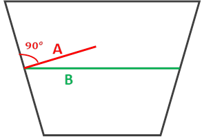
If wall adhesion is used with the contact angle of 90 degrees (A), then the boundary condition of the contact angle forces the interface to be normal to the boundary in the curvature calculation.
If wall adhesion is not used (B), then for the curvature calculation, the volume fraction gradient at the wall is copied from the cells adjacent to the wall, and there is no boundary condition enforcement of the contact angle.
To include wall adhesion in your model, refer to Including Surface Tension and Adhesion Effects in the User's Guide.
Similar to wall adhesion, there is also an option to provide jump adhesion when using the VOF model. Here, the contact angle treatment is applicable to each side of the porous jump boundary by assuming the same contact angle at both the sides.
Therefore, if  is the contact angle
at the porous jump, then the surface normal at the neighboring cell
to the porous jump is
is the contact angle
at the porous jump, then the surface normal at the neighboring cell
to the porous jump is
 | (14–35) |
where  and
and  are the unit vectors normal and tangential to the
porous jump, respectively.
are the unit vectors normal and tangential to the
porous jump, respectively.
To include jump adhesion in your model, refer to Steps for Setting Boundary Conditions in the User's Guide.
Ansys Fluent provides two methods of jump adhesion treatment at the porous jump boundary:
Constrained Two-Sided Adhesion Treatment:
The constrained two-sided adhesion treatment option imposes constraints on the adhesion treatment. Here, the contact angle treatment will be applied to only the side(s) of the porous jump that is(are) adjacent to the non-porous fluid zones. Hence, the contact angle treatment will not be applied to the side(s) of the porous jump that is(are) adjacent to porous media zones. If the constrained two-sided adhesion treatment is disabled, the contact angle treatment will be applied to all sides of the porous jump.
Note: This is the default treatment in Ansys Fluent.
Forced Two-Sided Adhesion:
Ansys Fluent allows you to use forced two-sided contact angle treatment for fluid zones without any imposed constraints. Refer to Steps for Setting Boundary Conditions in the User’s Guide to learn how to apply this option.