


This section describes how to use Ansys Fluent modeling capabilities based on the multi-scale multi-domain (MSMD) method. Only the procedural steps related to battery modeling are shown here. For information about inputs related to other models used in conjunction with the battery model, see the appropriate sections for those models in the Ansys Fluent Fluent User's Guide. For more details on the modeling approach, refer to Battery Model in the Fluent Theory Guide.
Information about using the model is presented in the following sections:
- 31.2.1. Limitations
- 31.2.2. Geometry Definition
- 31.2.3. Setting up the Battery Model
- 31.2.4. Using Parameter Estimation Tools
- 31.2.5. Initializing the Battery Model
- 31.2.6. Modifying Material Properties
- 31.2.7. Solution Controls for the MSMD Battery Model
- 31.2.8. Predefined Report Definitions for the Battery Model
- 31.2.9. Postprocessing the MSMD Battery Model
Note the following limitations when using the MSMD Battery model:
For battery pack simulations, all batteries in the pack must be identical initially, having the same battery type with the same initial conditions.
For battery pack simulations, all batteries in the pack must have the nPmS connection pattern; that is, n batteries connected in parallel, and then m such units connected in series.
A conductive zone must be continuous. Disconnected zones cannot be grouped as one entity.
System positive and negative tabs must be continuous surfaces. Disconnected faces cannot be grouped together as one entity.
The positive and negative tabs must be connected by either the real tab/busbar conductive volumes or the virtual connections defined through a file.
In the MSMD and Cell Network frameworks, the negative and positive current collectors, anode, and cathode are not resolved, and the battery is regarded as a homogeneous body. The computational mesh does not have to be adjusted to all layers present in the battery domain. The following zones have to be identified when creating the battery mesh:
Cell
Tab
Busbar (for battery pack cases with real battery connections)
Electro-chemical reactions occur in cell zones, which are defined in the Active Components selection list in the Battery Model dialog box (Conductive Zones tab). Tab and busbar zones only conduct electric current and are defined in the Passive Components selection list. See Specifying Conductive Zones for details.
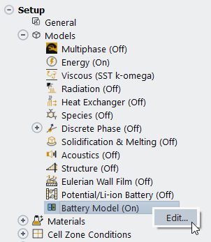
To enable the battery model, in the Outline View under the Models branch, right-click Battery Model and click Edit... in the menu that opens.
![]() Setup → Models →
Battery Model
Setup → Models →
Battery Model ![]() Edit...
Edit...
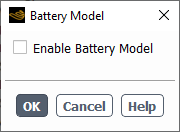
In the Battery Model dialog box that opens, select the Enable Battery Model check box to activate the model.
The Battery Model dialog box expands to reveal additional model options and solution controls.
The inputs for the battery model are entered using the following tabs:
- Model Options
contains the general model settings to define problems using the battery model.
- Conductive Zones
allows you to select zones for the active, tab and busbar components.
- Electric Contacts
allows you to define the contact surface and external connectors.
- Model Parameters
is where you specify the parameters to be used for solving the model equations.
- UDF
is where you can hook your user-defined functions.
- Advanced Options
allows you to quickly check the selected electrochemical submodel behavior in a standalone mode, and also to use various advanced modeling capabilities. See Specifying Advanced Options for more information.
Note: When setting up the model, you can click the Apply button to save your input values and your choices for your model. To restore the last saved settings for all tabs, click the Reset button.
For additional information, see the following sections:
- 31.2.3.1. Specifying Battery Model Options
- 31.2.3.2. Specifying Conductive Zones
- 31.2.3.3. Specifying Electric Contacts
- 31.2.3.4. Specifying Battery Model Parameters
- 31.2.3.5. Hooking User-Defined Functions
- 31.2.3.6. Specifying Advanced Options
- 31.2.3.7. Specifying External and Internal Short-Circuit Resistances
- 31.2.3.8. Setting a Battery Swelling Case
In the Model Options tab, you can select the electrochemical battery submodel and set various model options, solution controls, and electrical parameters.
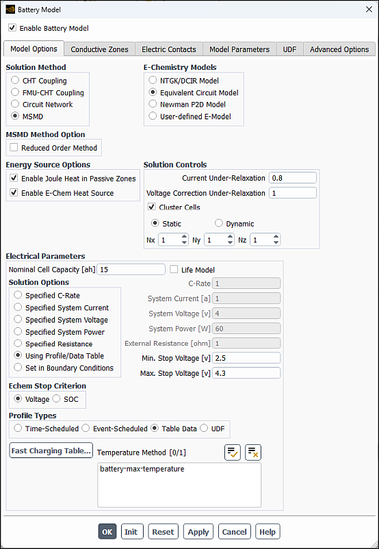
Select the solution method.
For Solution Method, if you select:
CHT coupling: A uniform heat source will be distributed within each battery's active zone. You need to specify the heat source directly. None or one potential equation will be solved, depending on whether Joule heating in passive zones is included or not. See CHT Coupling Method in the Fluent Theory Guide for more information about this method.
FMU-CHT coupling: A uniform heat source will be distributed within each battery's active zone. The heat source is computed from the functional mockup unit (FMU). None or one potential equation will be solved, depending on whether Joule heating in passive zones is included or not. See FMU-CHT coupling method in the Fluent Theory Guide for more information about this method.
Circuit Network: A uniform heat source will be distributed within each battery's active zone, the heat source is computed from an electric circuit network in Fluent. None or one potential equation will be solved, depending on whether Joule heating in passive zones is included or not. See Circuit Network Solution Method in the Fluent Theory Guide for more information about this method.
MSMD: If the Reduced Order Method option is not enabled in the MSMD Method Option group box, two potential equations will be solved during each iteration in the simulation. See MSMD Solution Method in the Fluent Theory Guide for more information about this method.
If you want to obtain a faster solution, select Reduced Order Method in the MSMD Method Option group box. This will enable the solver to run faster using the reduced order method (ROM). You can use this option if the two conditions listed in Reduced Order Solution Method (ROM) are met. Note that, prior to using the ROM, you must first run a simulation without this option for at least three time steps. Ansys Fluent will use these results as reference potential fields for the ROM method.
If you have selected Circuit Network or Reduced Order Method, set Number of Sub-Steps/Time Step. Using this value, you can specify the ratio of the time steps for thermal and electro-chemistry calculations. For example, if the Number of Sub-Steps/Time Step is set to
10, the solver will use one tenth of the CFD time step for the electro-chemistry calculation.Important: The internal short circuit treatment requires two potential equations to be solved. For this reason, it can only be used with the MSMD solution method, but not with the ROM method.
Select the electrochemistry model. The following submodels are available in Ansys Fluent under the E-Chemistry Models group box:
- NTGK/DCIR Model
is an empirical model. This is the simplest and the least expensive model. It also requires the fewest model inputs. The model uses the same NTGK method as that used by the Single-Potential Empirical model. However, in this case, it solves two potential equations continuously instead of one potential equation with a jump condition at the separator over all conductive zones. The model cannot accurately capture the battery's dynamic (inertial) response.
- Equivalent Circuit Model
is a semi-empirical model. It has limited capability for predicting the battery dynamic behavior.
- Newman P2D Model
is the most comprehensive physics-based battery model. It is computationally expensive, and it requires extensive user input of battery-related fundamental information.
- User-defined E-Model
is the user-specified electrochemical submodel. To be able to use this option in the Fluent MSMD method framework, you must provide the
void
           user_defined_echem_model()
function in the customizablecae_user.csource code file.
Optionally, you can enable the following Energy Source Options:
Enable Joule Heat in Passive Zones (default) in order to include the Joule heating source in the thermal energy Equation 19–3 in the battery passive conducting zones, including tabs and busbars,
Enable Joule Heat in Active Zones (default) in order to include the Joule Heating source in the thermal energy equation Equation 19–3.
Enable E-Chem Heat Source (default) in order to include the heat source due to electrochemistry in the thermal energy equation Equation 19–3.
Specify the following settings in the Solution Controls group box:
Set Current Under-Relaxation Factor. The volumetric current density used in the two potential equations are under-relaxed according to this factor. The default value of
0.8may be sufficient for most cases. The values in the range of 0.8–1.0 are recommended.Set Voltage Correction Under-Relaxation Factor. The default value of 1.0 is acceptable for most cases. You should reduce this value only if the convergence difficulty occurs during the solution of the potential equations.
(Equivalent Circuit Model and Newman P2D Model) Select the Cluster Cells check box to enable cell clustering and then define it using one of the following methods:
Static
When you select Static, you can specify the number of clusters Nx , Ny , and Nz in X, Y, and Z directions respectively. The solver will divide the active zone of every battery cell into Nx x Ny x Nz clusters and solve the electrochemical sub-model in each cluster using the cluster-averaging information.
The static clustering method is purely geometry-based. Clusters are formed before a simulation is run and they remain fixed in the simulation.
The default values for Nx , Ny , and Nz are 1, 1, and 1, respectively. For the initial run, the default settings are recommended.
Dynamic
When you select Dynamic, you can define the Number of Clusters and specify the Target Variable, which could be voltage or temperature. You can also define your own target variable by writing a
DEFINE_BATTERY_CLUSTERUDF. SeeDEFINE_BATTERY_CLUSTERin the Fluent Customization Manual for details.The dynamic clustering is done before the beginning of every time step and the clusters are formed dynamically during the simulation. The solver finds the range of the target variable in the active zone of a battery cell, and then divide this range into the specified number of clusters. Each control volume in the battery cell is grouped into a cluster according to its target variable value.
In the Electrical Parameters group box, specify the following operating conditions:
Set the Nominal Cell Capacity (the capacity of the battery cell).
If you want to model the battery capacity changes over time and over repeated discharging and charging cycles, enable the Life Model option and then set up the life model as described in Setting the Life Model.
For the Solution Options, you can:
Select Specified C-Rate and then specify C-Rate, which is the hourly rate at which a battery is discharged. A positive value means discharging C-rate and a negative value means charging C-rate. In this case, the total current at the cathode tabs is fixed as the product of C-Rate and Nominal Capacity, while the electrical potential is anchored at zero on the anode tabs. Note that the computation of current from the C-rate is always based only on the single battery's nominal capacity and does not account for the battery's connection information. For example, in a 2P2S module case, if you want to completely drain the fully charged module in one hour, you need to set the C-rate to 2.
Select Specified System Current and then specify System Current applied at the cathode tabs. A positive value means discharging current and a negative value means charging current.
Select Specified System Voltage and then specify System Voltage applied to the cathode tab. The anode tab has a voltage of 0 V.
Select Specified System Power and then specify System Power. If you specify the total power output from your battery, the Fluent solver will ensure that the product of the system current and voltage equals the system power. A positive value means discharging power output and a negative value means charging power input.
Select Specified Resistance and then specify External Resistance in an external short-circuit simulation. If you specify the external electric resistance in Ohm, the Fluent solver will ensure that the ratio of the system voltage to the system current equals the specified external resistance.
Select Set in Boundary Conditions and then set the UDS boundary conditions directly, for example, the voltage value or the current value (specified flux), using the Boundary Conditions task page in Ansys Fluent for the specific face zone.
Select Using Profile/Data Table and then specify a profile or data table as described in Specifying a Profile or Data Table.
For Echem Stop Criterion, you can:
Select the Voltage method and specify Min Stop Voltage and Max Stop Voltage, or
Select the SOC method and specify Min Stop SOC and Max Stop SOC.
In a battery simulation, the stop criterion is checked after every time step. For the voltage method, battery's cell voltage is checked against the minimum and maximum stop voltage. For the SOC method, the SOC level in a battery is checked. Once the stop criterion is met, the simulation stops automatically.
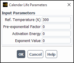
If you have selected the Life Model option (Electrical Parameters group box), you must specify the following life model parameters:
- Calender Time
is the storage time (
 in Equation 19–45 in the Fluent Theory Guide). You
can use any units that are consistent with the kinetics quantities you specify in the
Calendar Life Parameters dialog box (see Figure 31.3: The Calendar Life Parameters Dialog Box).
in Equation 19–45 in the Fluent Theory Guide). You
can use any units that are consistent with the kinetics quantities you specify in the
Calendar Life Parameters dialog box (see Figure 31.3: The Calendar Life Parameters Dialog Box).- Cycle Number
is the number of cycles that the battery has experienced so far (
 in Equation 19–46 in the Fluent Theory Guide).
- Operation Temperature
is the average temperature to which the battery has been exposed over time and over its previous discharging/charging cycle (
 in Equation 19–45 and Equation 19–46 in the Fluent Theory Guide). Note that this temperature is
not the same as the battery temperature during CFD simulations.
in Equation 19–45 and Equation 19–46 in the Fluent Theory Guide). Note that this temperature is
not the same as the battery temperature during CFD simulations.- Calendar Life Parameters
are the calendar-life-related parameters that can be specified in the Calendar Life Parameters dialog box that opens when you click the button.
The following Input Parameters are available:
Ref. Temperature: Is the reference temperature under which these kinetics parameters are obtained (
 in Equation 19–45 in the Fluent Theory Guide).
Pre-exponential Factor: Is
 in Equation 19–45 in the Fluent Theory Guide.
Activation Energy: Is
 in Equation 19–45 in the Fluent Theory Guide).
Exponent Value: Is the time exponent factor (
 in Equation 19–45 in the Fluent Theory Guide).
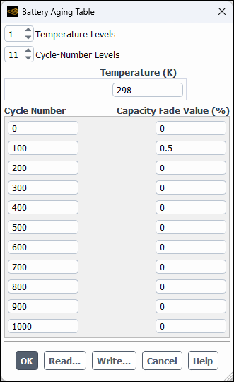
- Battery Aging Table
is a 2D lookup table for capacity fade factors at different temperatures and cycle numbers. All values are entered in the Battery Aging Table dialog box that opens by clicking the button (for example Figure 31.3: The Calendar Life Parameters Dialog Box).
For the NTGK model, you can specify the following inputs in the Battery Aging Table dialog box:
Temperature Levels
Cycle-Number Levels
Values of Temperature
Values of Cycle-Number
Capacity fade values for each cycle-temperature pair
You can specify up to 20 Temperature Levels and Cycle-Number Levels.
You can use the Write... button to store the 2D lookup table to a file in a text format, which you can use later by clicking the Read... button and using the Select File dialog box that opens. You can also generate your own 2D lookup text file and read it into Ansys Fluent. Both the compact scheme and the plain text format can be used when reading or writing a table from/to a file. Refer to Using Tables in the Battery Model for more information about these table formats. The capacity fade values will be automatically populated in the Battery Aging Table dialog box.
If you have select Using Profile/Data Table (Solution Options group box), you can use one of the following options in the Profile Types group box:
Time-Scheduled
Event-Scheduled
Table Data
This option can be used to specify a fast charging electric current profile as a 2D lookup table. Further details are provided below.
UDF
You can use the UDF option to define the electric load type and value using a
DEFINE_BATTERY_ELOAD_PROFILEUDF. The UDF option is used if the time-scheduled and event-scheduled profile cannot cover the profile you want to use. SeeDEFINE_BATTERY_ELOAD_PROFILEin the Fluent Customization Manual for information aboutDEFINE_BATTERY_ELOAD_PROFILE.
For the Time-Scheduled or Event-Scheduled options, you must provide time-dependent or event-dependent input (respectively) for the C-rate, current, voltage, or power. The time-scheduled and event-scheduled profiles enable you to change the electric load type and electric value in the simulation on the fly. When either the Time-Scheduled or Event-Scheduled profile type is selected, you can browse to the ASCII text file with either the .dat or .txt file extension that you generated beforehand. The inputs for the Time-Scheduled and Event-Scheduled profiles are described below.
Time-Scheduled Profile Specification
The Time-Scheduled profile file must be organized in three columns:
Time
Electric load value
Electric load type
The electric load type is defined by an integer number:
0: C-rate1: Current2: Voltage3: Power4: External electric resistance
For example, the below time-scheduled profile:
0        15    1
500      15    1
500.1    60    3
1000     60    3
1000.1   -1    0
1500     -1    0
specifies the following battery charging scenario:
The battery is discharged at 15 A for the first 500 seconds.
The battery discharge continues at 60 W for the next 500 seconds.
The battery is charged at a constant 1 C-rate for the last 500 seconds.
Note:
For current, power, or C-rate, a positive value means discharging and a negative value means charging.
The unit of the variables in the input file is always SI.
Ansys Fluent solver uses linear interpolation of your time-scheduled profile data in the problem simulation. If you want to capture a sudden change in the profile accurately, use smaller time gaps to describe the profile.
Event-Scheduled Profile Specification
The Event-Scheduled profile file must be organized in the following five columns:
Electric load type
Just as in the time-scheduled profile, the electric load type is defined by an integer number:
0: C-rate1: Current2: Voltage3: Power4: External electric resistanceElectric load value
Forwarding condition
The forwarding condition (FC) is defined by an integer number:
1: Time > FC_Value2: I < FC_Value (discharging current minimum)3: I > FC_Value (charging current maximum)4: V < FC_Value (system voltage minimum)5: V > FC_Value (system voltage maximum)6: P < FC_Value (discharging power minimum)7: P > FC_Value (charging power maximum)8: Time Duration > FC_Value (Time Duration)Forwarding condition value
Stop flag
The stop flag is an integer value of 0 or 1, where 0 specifies that the run should continue to the next event entry line, and 1 specifies that the run should end.
For example, the below event-scheduled profile:
0    1    4  3.5    0
0    0    8  300    0
1  -15    5  4.1    0
2  4.1    3   -1    1
specifies the following scenario:
The battery is discharged at 1 C rate until the voltage reaches 3.5 V.
The battery is at rest for 300 seconds.
The battery is charged at constant current 15 A until the voltage reaches 4.1 V.
The battery keeps charging at 4.1 V until the current is greater -1 A. The simulation stops after reaching this point.
Note:
For current, power, or C-rate, a positive value means discharging and a negative value means charging.
The unit of the variables in the input file is always SI.
Any time-scheduled profile can be rewritten in an event-scheduled profile format, but not vice-versa. The example shown in the time-scheduled profile can be redefined in an event-scheduled profile format as follows.
1    15    1    500    0
3    60    1   1000    0
0    -1    1   1500    1
Both profile types can be read into Ansys Fluent. You can choose the most convenient one to use in your specific application.
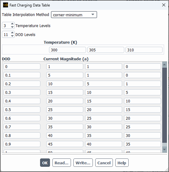
Table Data Specification
The fast charging 2D lookup table defines the charging current as a function of battery's average DOD and temperature. To use this specification method follow the steps below:
Create one or more report definitions of temperature.
In the Temperature Method list, select the report definition(s) to be used in the lookup table.
The lookup table will be searched for all selected temperature definitions, and the minimum value will be used as the charging current.
Click
In the Fast Charging Data Table dialog box that opens, specify the following inputs.
Select the Table Interpolation Method from the following options:
bilinear
The bilinear interpolation method is used to find charging current value given a DOD and a temperature value.
staircase-floor
For a given temperature, the current changes as a staircase and the lower DOD value is used. Linear interpolation is used for temperature.
staircase-ceiling
The DOD ceiling value is used. Linear interpolation is used for temperature.
corner minimum
The lowest conner value is used from the lookup table.
The interpolated value for charging current are different for different methods. The example below shows the charging current data for two temperature levels of and two DOD levels.
T=300 K T=310 K DOD=0.2 10 5 DOD=0.3 20 10 The interpolated value of charging current for T=305K and DOD=0.25 will be:
Bilinear: Charging Current = ((20+10)/2+(5+10)/2)/2= 11.25
Staircase-floor: Charging Current = (10+5)/2 =7.5
Staircase-ceiling: Charging Current = (20+10)/2 = 15
Corner-minimum: Charging Current = 5
Enter values for the following table parameters:
Temperature Levels
DOD Levels
Values of Temperature
Values of DOD
values of Current Magnitude for each DOD level and temperature
2D and 3D lookup tables are used in the battery model to specify various quantities as tabular functions of other solution variables when the tabular input option is available. Lookup tables are tab- or space-delimited ASCII text files that support the following formats:
Plain text format (files with extension .txt)
A 2D table must contain the following entries:
Row 1 – Header keyword “
x-values”Row 2 - x-value points
Row 3 – Header keyword “
y-values”Row 4 - y-values points
Row 5 – Header keyword “
table-values”Row 6 and all consecutive rows - table input data
An example of the 2D table for capacity fade factors at two temperature levels and three cycles-number levels is shown below:
x-values
   300   310
y-values
     0   100   200
table-values
     0     0
   0.1  0.15
   0.2  0.25
A 3D table is used only for specifying internal resistance data. For each electric current level, a 2D table of resistance values at different temperature and DOD levels must be provided. The table must include the following data:
Keyword “
z-value” followed by a current value at the first electric current level2D table for the first electric current level. see the description above of 2D tables
Keyword “
z-value” followed by a current value at the second electric current level2D table for the second electric current level
Etc.
An example of the 3D table is shown below:
z-value  -10
x-values
   300   310
y-values
     0   0.5   1.0
table-values
   111   112
   121   122
   131   132

z-value  0
x-values
   300   310
y-values
     0   0.5   1.0
table-values
   211   212
   221   222
   231   232

z-value  10
x-values
   300   310
y-values
     0   0.5   1.0
table-values
   311   312
   321   322
   331   332
Compact scheme format (files with extension other than .txt, for example .tab)
In this format, each data group is enclosed in parentheses, and the input values within each group are separated by spaces and/or tabs.
In the following example, the same 2D table for capacity fade factors shown above is written in the compact format:
((300 310) (0 100 200) ((0 0) (0.1 0.15) ( 0.2 0.25)))
The first group of numbers
(300 310)contains x-value points, which are the temperature levels. The second group of numbers(1 100 200)contains y-value points, which are the cycle numbers. The third group contains table entry values where each sub-group in parentheses represents a row of data in the table.The 3D table containing internal resistance data shown in the example above can be written in the compact format as follows:
((-10 0 10) (((300 310) (0 0.5 1.0) ((112 112) (121 122) (131 132)))
             ((300 310) (0 0.5 1.0) ((212 212) (221 222) (231 232)))
             ((300 310) (0 0.5 1.0) ((312 312) (321 322) (331 332)))) 0)
The first group of data
(-10 0 10)contains three electric current values. The second group includes three 2D lookup tables for the three electrical current levels. In each 2D table, the temperature array is listed first, followed by the DOD array and then by the resistance values for each temperature-DOD pair. The last digit in the list indicates the interpolation method.0denotes the bilinear interpolation, which must always be used for this particular table.
Usually if you transfer table data from one simulation to another, you can use the compact scheme format. If you prepare table data manually through a file, the plain text format is more readable and may be a better choice.
The Conductive Zones tab of the Battery Model dialog box allows you to specify the active, tab, and busbar zones.
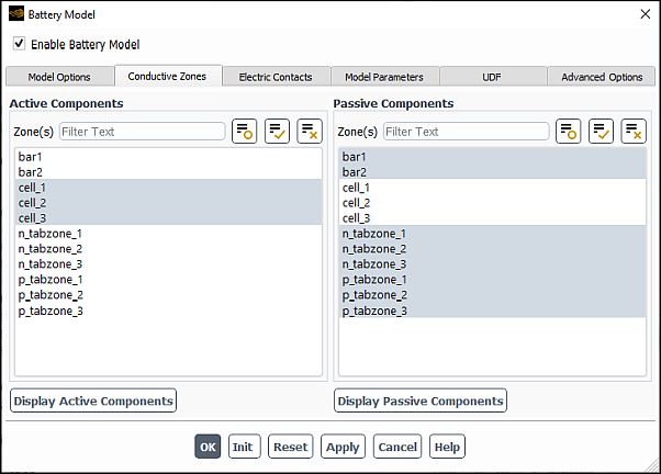
In the Conductive Zones tab, select the appropriate zones for the Active Components and Passive Components. Passive components include battery tab zones and busbars used to connect tabs of different batteries. You can visualize all active or passive zones by using the Display Active Components or Display Passive Components button, respectively. This opens the Mesh Display dialog box where all relevant components are selected automatically.
Battery cells are modeled as active zones; and battery tabs and busbars are modeled as passive zones. Electrochemical reactions occur only in the active zones. The potential field is solved in both active and passive zones.
The Electric Contacts tab of the Battery Model dialog box allows you to set the properties of the Contact Surfaces and the External Connectors.
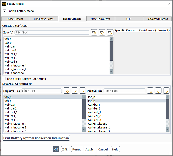
If you want to consider contact resistance, select zones for the Contact Surfaces and set the Specific Contact Resistance for any selected contact surface.
When using real connections, define the system negative and positive tabs under External Connectors.
When using the virtual connection option in a battery pack simulation, select the Use Virtual Battery Connection check box and in the Specify connection file text-entry box that appears, enter the filename containing the virtual connection definition.
The following input formats can be used:
tab surface-based format
active zone volume-based format
The tab surface-based format for the connection definition file is as follows:
mP 2
nS 2
tab_N_1P1S  tab_P_1P1S
tab_N_2P1S  tab_P_2P1S
tab_N_1P2S  tab_P_1P2S
tab_N_2P2S  tab_P_2P2S
where:
The first line specifies the number of parallel batteries in a stage (mP).
The second line specifies the number of stages in series in a pack (nS).
The remaining lines contain pairs of the face names of the negative and positive tabs for each battery. The battery data are listed in the following order: 1P1S ... mP1S to 1PnS ... mPnS.
For the above battery connection file example, the battery solver establishes the 2P2S connection pattern.
The following figure shows the different resulting connection patterns for the different connection data.
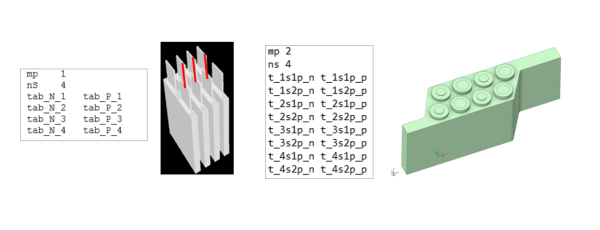
Once all conductive zones and the positive and negative tabs have been defined, Ansys Fluent automatically detects the battery network connection.
The active zone volume-based format for the connection definition is as follows:
mP	1
nS	4
cell_1
cell_2
cell_3
cell_4
where:
The first line specifies the number of parallel batteries in a stage (mP).
The second line specifies the number of stages in series in a pack (nS).
The remaining lines contain the names of the active battery zones in the order of: 1P1S ... 1PnS to mP1S ... mPnS.
You should use one line only for each battery. If a battery active zone includes multiple cell volumes, list all of them in one line separated by space, for example:
mP	1
nS	4
cell_1_a   cell_1_b    cell_1_c
cell_2
cell_3_a   cell_3_b    cell_3_c
cell_4
Note: The active zone volume-based connection file can only be used for cases that involve the Circuit Network solution method without the Joule heating effects. This is because the electric current flow passage is not determined in a battery pack. Consequently, the potential field, and therefore the Joule heating effect, cannot be solved.
When you import either format of the connection file, Ansys Fluent automatically detects the type of the format. If the active zone volume-based format is used, the solver enables the Circuit Network solution method and disables the Joule heating effects. The zones in the active and passive components listed under the Conductive Zones tab are updated automatically according to the information provided in the connection file.
After you have defined all the conductive zones or modified zone related data, click Print Battery System Connection Information, and review the battery connection information printed in the Ansys Fluent console window for any errors. If necessary, re-define the connections in the Conductive Zones and Electric Contacts tabs.
The Model Parameters tab of the Battery Model dialog box allows you to specify the submodel-specific parameters. The Model Parameters tab contains only the entry fields for parameters related to either the solution method or electrochemical submodels you have chosen in the Model Option tab. A detailed description of inputs for each submodel is given in the sections that follow.
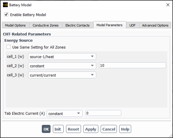
You need to specify the following CHT-Related Parameters:
total Energy Source for each battery active zone
(if you want to consider the Joule heating in passive zones) Tab Electric Current
For both heat source and tab electric current, you can use either constant data type or any of the imported transient profiles.
If constant is selected, you need to specify a value in the adjacent field.
To use transient profiles for energy sources, you first need to read all profile files into your simulation as outlined in Reading Profile Files. Once the profiles have been imported into your analysis, their names automatically appear in the drop-down lists for each active zone and for tab electric current. The profile file format conforms to the Ansys Fluent built-in transient profiles described in Transient Cell Zone and Boundary Conditions. The below example shows the file format of a tabular transient profile (.ttab).
energy-source  2  4  0
time       energy-source
0          5.0
100        5.0
100.1      10.0
10000      10.0
In this example, the first line contains the profile name, followed by the number of fields, the number of lines, and the flag indicating whether the profile is periodic.
The second line contains all the field names. One of the field names must be
time for the profile to be correctly recognized.
The remaining rows contain the profile data.
All the imported profiles will be saved within the Ansys Fluent case file.
If in a pack simulation, the same heat source is used for all active zones, you can select Use Same Settings for All Zones and define only one set of data. Ansys Fluent will automatically update all zones with the same cell information.
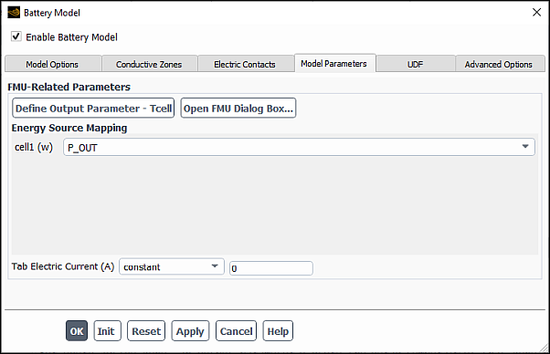
In the FMU-Related Parameters group box, click the Define Output Parameter- Tcell button.
Fluent creates an output parameter, the average zone temperature, for each active zone.
Click Open FMU Dialog Box... and then use the cell average temperatures that have been generated in the previous step to define the FMU input parameters in the Parameters dialog box. Refer to Coupled Simulations in Ansys Fluent with Functional Mock-up Unit (FMU) Files for details on the FMU file importing procedure.
Once the FMU file importing is complete, you can define the following parameters:
For each battery active zone, under Energy Source Mapping, select an appropriate FMU output parameters that have been imported in the previous step to be an energy source term.
If the Joule heating is considered, specify Tab Electric Current. Similar to the CHT Coupling solution method, you can choose either constant or any of the imported transient profile. See Inputs for the CHT Coupling Method for more information.
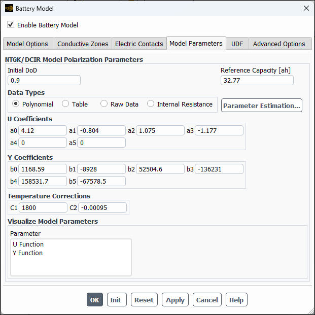
For the NTGK/DCIR Model, define the following operating conditions:
Specify the following NTGK model parameters:
Initial DoD: Is the battery initial DOD at
 =0. The default value of
 0for Initial DoD indicates the fully-charged state of the battery cell.Reference Capacity: Is the capacity of the battery that is used in experiments to obtain the model parameters (
 in Equation 19–5).
Nominal and reference capacities may have different values.
in Equation 19–5).
Nominal and reference capacities may have different values.
Specify
 and
and  model parameters in Equation 19–7 using one of the following:
 Polynomial data type
Table data type
Raw Data data type
Parameter Estimation tool
or directly define the battery internal resistance by using the Internal Resistance data type.
If you selected Polynomial in the Data Types group box, enter polynomial coefficients for
 ,
,  , and temperature correction in Equation 19–7 directly in the U Coefficients and
Y Coefficients group boxes.
, and temperature correction in Equation 19–7 directly in the U Coefficients and
Y Coefficients group boxes.If you selected Table in the Data Types group box, define a 2D lookup table for each NTGK model parameter.
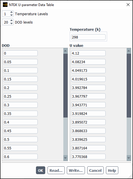
Tabular data are entered in the corresponding parameter data table dialog box that opens by clicking the relevant button (U Table... or Y Table...) in the NTGK Parameter Data Table group box (see Figure 31.11: NTGK U-parameter Data Table Dialog Box).
For each NTGK model parameter, you can specify up to 50 DOD levels and 20 temperature levels. For each DOD-temperature pair, you must enter the corresponding model parameter value. Each table can be exported to or imported from a file by clicking Write or Read, respectively, in the parameter data table dialog box. Both the compact scheme and the plain text format can be used when reading or writing a table from/to a file. Refer to Using Tables in the Battery Model for more information about these table formats.
Note: The model parameters for the NTGK Model Polarization Parameters are based on battery cell polarization test curves. Obtaining model parameters (other than the default values) can be dependant on your battery configuration and material properties. The default values are taken from Kim’s paper 313. If you model a battery having a different design, you must provide a different set of battery parameters.
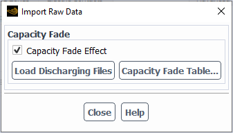
If you selected Raw Data in the Data Types group box, you need to import a set of testing data (discharging curves under different temperature and C-rate) by clicking the button.
In the Import Raw Data dialog box that opens, you can import testing data files by clicking the button and then using the Select File dialog box to read the files into your Fluent case.
If you want to include the capacity fade effect into your simulation, enable Capacity Fade Effect. After you import the testing data, the capacity fade table is populated automatically. You can review the table by clicking Capacity Fade Table..., but you cannot modify it.
Each capacity fade factor in the capacity fade table is computed from the test data as:
After you import test data files, no other information is needed. The Ansys Fluent solver stores the
U~Irelationship from the test data and will use it during the battery simulation.Note: The raw data treatment depends on whether the capacity fade effect is included or not. If you enable or disable the Capacity Fade Effect option, you need to load the data files again to re-process it.
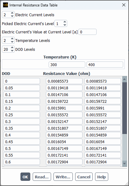
If you selected Internal Resistance in the Data Types group box, you need to define the internal resistance table and specify other parameters in the DCIR Method Settings group box.
Click the button.
In the dialog box that opens, enter the table data.
Specify the number of Electric Current Levels.
Set the Selected Current Level for which you want to define internal resistance points.
Enter a value for the Current for the selected current level.
Specify values for the following table parameters:
Temperature Levels
DOD Levels
Values of Temperature
Values of DOD
Values of Current Magnitude for each DOD level and temperature
A positive value means discharging current and a negative value means charging current. In this way, you can use different internal resistance when simulating charging and discharging.
Repeat steps 2 through 4 for each current level.
You can write a table data into a file or fill the table by importing data from a file. Both the compact scheme and the plain text format can be used when reading or writing a table from/to a file. Refer to Using Tables in the Battery Model for more information.
If you want to include the open circuit potential, enable U Table, click the U Table... button, and in the NTGK Parameter Data Table dialog box that opens (see Figure 31.11: NTGK U-parameter Data Table Dialog Box), enter U values for each DOD-temperature pair.
Note: If the U-table is not provided, you can use only either the current or C-rate electrical load condition. In addition, only single battery or pure serial battery connection can be simulated.
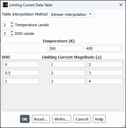
(cases with no fast charging) If you want to limit current in your simulation, perform the following steps:
Enable Limiting Current.
In the Temperature Method list, select the report definition(s) to be used in the lookup table.
Click the Current Limiting Table... button.
In the Limiting Current Data Table dialog box that opens, specify a 3D table of the limiting current values.
The inputs are similar to those in the Fast Charging Data Table dialog box described in Specifying a Profile or Data Table.
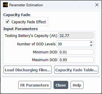
If you want to use the parameter estimation tool to fit
and from testing data, click the Parameter Estimation...
button.In the Parameter Estimation dialog box that opens, you need to specify the following Input Parameters:
Testing Battery's Capacity
This value is copied from the Reference Capacity (Model Parameters tab). You need to verify it is correct; otherwise, go back to the Model Parameters tab to modify it.
Number of DOD Levels
The number of DOD levels is a number between 10 and 20. The default 20 is a good choice for all cases. The required discharging data are battery's discharging curves at different constant C-rates. You can use testing data at different temperatures. For each C-rate, you must provide a separate file in text format. At least two input files with data at different C-rates are required to get meaningful fitting results.
Minimum DOD: Minimum battery's DOD level used in the fitting. The default value is 0.01, which is suitable for most cases.
Maximum DOD: Maximum battery's DOD level used in the fitting. The default value is 0.95, which is suitable for most cases.
Corresponding discharging data (as further described)
If you want to consider the capacity fade effect in your simulation, enable Capacity Fade Effect.
After the parameter fitting process is complete, the capacity fade table is populated automatically. You can review the table by clicking Capacity Fade Table..., but you cannot modify it. The fitting results (
and parameters) are dependent upon whether the capacity fade effect is
considered or not. If you have modified the state of Capacity Fade
Effect, you need to re-fit the model parameters.To import all the testing files, click the Load Discharging Files button and use the Select File dialog box that opens to read multiple testing data files. The selected testing files will be listed at the bottom of the Select File dialog box. If you accidentally select the wrong file, you can use the Remove button to remove it from the selected testing file list.
An example of an input file is shown below.
Crate 1.0
Temperature 300.0
1.0000e+00   4.1097e+00
2.0000e+00   4.1094e+00
3.0000e+00   4.1092e+00
...
3.6000e+01   4.1010e+00
...
The first line of the file starts with
Cratefollowed by a C-rate value separated by a space. The second line starts withTemperaturefollowed by a value. The lines that follow contain pairs of space-separated time-voltage values.After testing files are imported, click the Fit Parameters button to run the NTGK parameter estimation tool.
If you provide testing data files at different temperatures, the parameter estimation tool will perform the fitting for each temperature level. Ansys Fluent will report the fitted results in the console and automatically pass them in a table data type to the parameter data table dialog boxes. The Table data type will be automatically selected in the Battery Model dialog box. This will allow you to consider the temperature-dependent effect.
If you use testing data from only one temperature level, the fitting results in both polynomial and table data types will be filled in the Battery Model dialog box. In this case, the Polynomial data type is the default data type. However, you can use either data type in your simulation.
(optional) Visualize and check the resulting fitted curves of the battery discharge data at different temperatures and C-rates to detect any issues with the fitting process.
Once the fitting is complete, the Parameter Estimation dialog box expands to reveal the Visualize Fitting Results group box containing the Temperature and C rate selection lists. You can display curves of the fitted discharge data and the experimental data from your input files at different temperatures and C-rates by selecting a pair of desired values from the Temperature and C rate lists. The corresponding curves will be automatically plotted in the graphics window.
Click Close in the Parameter Estimation dialog box.
Note: The NTGK parameter estimation tool can also be accessed through the text user interface (TUI) as described in Using the Parameter Estimation Tool for the NTGK Model in the TUI.
(Polynomial or Table data type only) You can visualize the resulting
and parameters varying with DOD by selecting U Function
or Y Function from the Parameter list
(Visualize Model Parameters group box) and clicking the
Plot button. The resulting curves at temperatures you provided will be
plotted in the graphics window.

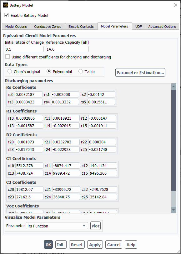
For the Equivalent Circuit Model (ECM), define the following operating conditions:
Specify the following Equivalent Circuit Model parameters:
Initial State of Charge: Is the battery initial SOC at
=0. The default value of 1for Initial State of Charge indicates the fully-charged state of the battery cell.Reference Capacity: Is the capacity of the battery that is used in experiments to obtain model parameters (
 in Equation 19–9). Note
that nominal and reference capacities may have different values.
in Equation 19–9). Note
that nominal and reference capacities may have different values.
Specify resistors' resistances (Rs, R1, and R2), capacitors' capacitances (C1 and C2), and the open circuit voltage (Voc) using one of the following:
Chen's original data type
Polynomial data type
Table data type
Parameter Estimation tool
Note: The values of model parameters for the Equivalent Circuit Model are battery specific and need to be specified before conducting a simulation. The default values are taken from Chen (see ECM Model for details). If you model a battery of different design, you should specify a different set of battery parameters.
If you selected Chen's original in the Data Types group box, you need to specify all coefficients in Equation 19–11.
If you selected Polynomial in the Data Types group box, you need to directly specify polynomial coefficients in Equation 19–10.
If you selected Table in the Data Types group box, you need to define a 2D lookup table for each ECM parameter. See Inputs for the NTGK/DCIR Model for more information on how to define model parameters in a table data type.
(optional) You can enable the Use Different Coefficient for Charging and Discharging option and specify the coefficients for charging parameters.
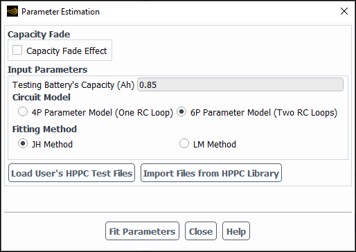
If you want to use the parameter estimation tool to fit the parameters from testing data, click the Parameter Estimation button.
In the Parameter Estimation dialog box that opens, you need to specify the following Input Parameters:
Testing Battery's Capacity
This value is copied from Reference Capacity (Model Parameters tab). You need to verify it is correct; otherwise, go back to the Model Parameters tab to modify it.
Circuit Model (4P Parameter Model (One RC Loop) or 6P Parameter Model (Two RC Loop))
Fitting Method (JH or LM Method)
The Jiang-Hu (JH) method uses only the testing data from the relaxation time period, and the Levenberg-Marquardt (LM) method uses the testing data from both the pulse and relaxation time periods. The JH method uses the approach from paper [69], and the LM method uses the general Levenberg-Marquardt method.
Corresponding HPPC testing data (as further described)
If you want to consider the capacity fade effect in your simulation, enable Capacity Fade Effect.
If this option is enabled, you need to import HPPC testing files for the discharging curves. The format of the discharging curve is the same as used for the NTGK parameter estimation tool. After you load files for the discharging curves, the capacity fade table is populated automatically. You can review the table by clicking Capacity Fade Table..., but you cannot modify it.
Load HPPC files into your case.
The required testing data are battery's HPPC data at different SOC and temperature. For each SOC and temperature level, you must provide a separate file in text format.
At least one valid SOC level testing data is required per temperature level. For good simulation results, the range of SOC levels used in the testing should cover the SOC range simulated in the CFD runs.
The file format must follow the format as shown in the below example:
SOC 1.0
I   14.6
Temperature 300.0
1.0000e-01    4.2292e+00
2.0000e-01    4.2292e+00
...
1.1800e+01    4.1041e+00
...
The first line of the file starts with
SOCfollowed by a SOC value separated by a space. The second line contains the pulse current information (Ifollowed by a pulse current value). The third line provides temperature information (keywordTemperaturefollowed by a value). The remaining lines contain pairs of space-separated time-voltage values. The input data must include data from the rest period, the pulse period, and the relaxation period in the testing.You can load HPPC files in one of the following ways:
If you have data from the battery's HPPC test, you can load them into your case by clicking the button.
In the Select File dialog box that opens, browse to the directory where the test files reside.
Select all the files obtained from different temperature and SOC levels you want to use in the parameter estimation tool (use Ctrl or Shift to select multiple files).
The selected testing files will be automatically added to the list of the files at the bottom of the Select File dialog box. If you accidentally selected the wrong file, you can use the button to remove it from the selected testing file list.
Click .
See The Select File Dialog Box for details.
You can load test files from the HPPC library provided by Ansys Fluent by clicking the button.
In the HPPC Data Library dialog box that opens, you can select a library from the Available Library List. The related information is displayed in the Summary of Library Information group box. Clicking will import the library files into your case.
See The HPPC Library for more information.
After testing files are imported, click the Fit Parameters button to run the ECM parameter estimation tool. The fitting results will be passed to the Battery Model dialog box automatically.
If you provide testing data files at different temperatures, the parameter estimation tool will perform the fitting for each temperature level. Ansys Fluent will report the fitted results in the console and automatically pass them in a table data type to the parameter data table dialog boxes. The Table data type will be automatically selected in the Battery Model dialog box (Model Parameters tab). This will allow you to consider the temperature-dependent effect.
If you use testing data from only one temperature level, the fitting results in both polynomial and table data types will be transferred to the Battery Model dialog box and to the parameter data table dialog boxes, respectively. In this case, the Polynomial data type will be automatically selected as default in the Battery Model dialog box. However, you can use either data type in your simulation.
If your testing data contains both discharging and charging curves, the ECM parameter estimation tool will be run twice—once for the discharging curves, and once for the charging curves. After the fitting is complete, the Use Different Coefficient for Charging and Discharging button will be automatically selected, and the fitting results for each subset of data will be automatically transferred to the Battery Model dialog box and displayed in the corresponding Discharging Parameters and Charging Parameters group boxes (Model Parameters tab).
Note:Because the parameter estimation tool attempts to calculate six or four ECM model parameters from a non-linear data regression process for each SOC curve, the testing data for each SOC curve should be sufficiently large in order to obtain a good fitting.
The parameter estimation tool always fits the experimental data into either six parameters used in the Chen's circuit shown in Figure 19.1: Electric Circuits Used in the ECM Model or four parameters in the reduced Chen's circuit with only one RC loop.
To obtain optimal fitting of HPPC testing data, you can try different combinations of the circuit model and the fitting method. The six-parameter circuit model has more physics, but the four-parameter circuit model is generally more robust. As for the fitting method, the JH method is in general more robust than LM method. You can start with the six-parameter model, and then, if the fitting results are not satisfactory, switch to the four parameter model.
(optional) Visualize and check the resulting fitted curves of the battery HPPC data at different temperatures and SOC to detect any issues with the fitting process.
Once the fitting is complete, the Parameter Estimation dialog box expands to reveal the Visualize Fitting Results group box containing the Temperature and State of Charge selection lists. You can display curves of the fitted data and the experimental data from your input files at specific temperatures and C-rates by selecting a pair of values from the Temperature and State of Charge lists. The corresponding curves will be automatically plotted in the graphics window.
When the data contains both discharging and charging curves, you can select either Discharging Data or Charging Data to visualize the corresponding subset of data. The Temperature and State of Charge lists will be updated accordingly.
Note the following when you are using the LM fitting method:
The LM method is a non-linear fitting method. To have a better fitting result with this method, the JH method is always run first to provide an initial condition for the fitting parameters. When you plot fitted curves, the fitting result from the JH method will also be plotted for your reference.
If the fitting fails, a warning message will be printed in the console window, and the fitted curve for the LM method will not be plotted.
Click Close in the Parameter Estimation dialog box.
Note: The ECM parameter estimation tool can also be accessed through the text user interface (TUI) as described in Using the Parameter Estimation Tool for the ECM Model in the TUI.
(Chen's original, Polynomial, or Table data type only) You can visualize the resulting resistors' resistances (Rs, R1, and R2), capacitors' capacitances (C1 and C2), and the corresponding time constants (R1*C1 and R2*C2) varying with DOD by selecting an appropriate function from the Parameter drop-down list (Visualize Model Parameters group box) and clicking the Plot button. The resulting curves will be plotted in the graphics window.
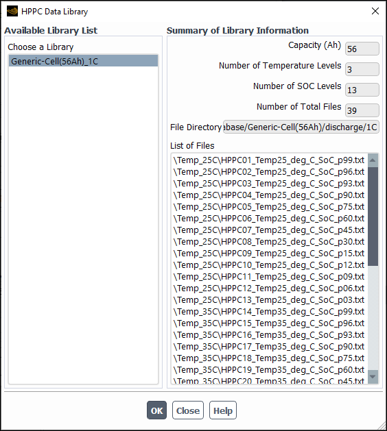
Ansys Fluent provides a small HPPC library that you can use for importing HPPC test data into your case. Currently, the library contains only a single battery, called Generic-Cell. In future releases, the library will be expanded to include commonly used batteries. The purpose of the Generic-Cell library is to show the folder structure of test files as further described.
The Ansys Fluent HPPC library is located in the following directory:
path/fluent24.2.0/addons/msmdbatt/hppc_database/
where
path
is the Ansys Fluent installation
directory (for example, C:\Program Files\ANSYS
Inc\v242\fluent\fluent24.2.0).
In a standard HPPC test, a pulse of current is applied to a battery at a particular temperature and SOC level, and the voltage response of the battery is measured. The voltage response curve depends on:
the nature of the pulse (discharging or charging)
the magnitude of the current
the temperature level
the SOC level of the battery
To reflect such testing procedure, the test files are organized in the folder structure as shown in Figure 31.19: Overview of the Folder Structure in the HPPC Library.
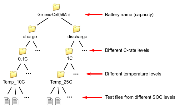
The naming convention is as follows:
The battery name can be any string. The capacity of the battery must be put in the parenthesis with a number followed by the unit "Ah".
The names of the first-level folder must be discharge and charge.
The number of the second- and third-level folders and their names can be arbitrary.
You can create your own library following the outlined conventions and put it in the hppc_database folder. The name of your library will appear in the HPPC Data Library dialog box. This way, the HPPC library can be expanded with the proprietary data and shared between colleagues within an organization.
Note: Currently, the parameter estimation tool can only take data from the discharge branch and only handle data from one C-rate level. Data from different C-rate levels are treated as different battery libraries. You should select the library with the C-rate level close to that at which the battery is operating in your application. The charge branch is not used so far. However, support for the charge branch is expected in future releases as the solver capability will be expanded in Ansys Fluent.
Theoretical Capacity is computed automatically from the Newman input parameters you specify and reported in the Model Parameters tab.
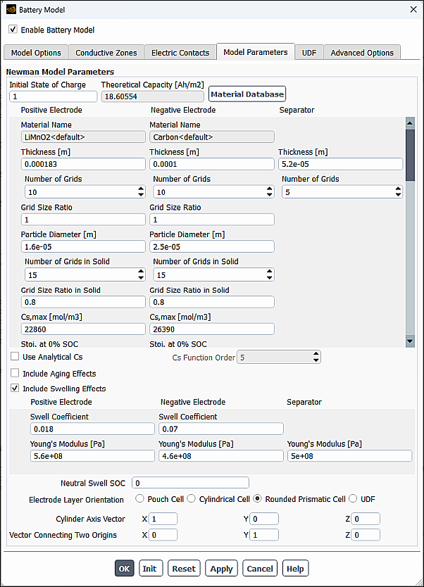
Specify the following settings in the Model Parameters for the Newman’s P2D model:
Specify Initial State of Charge. The default value of
1for Initial State of Charge indicates the fully-charged state of the battery cell.Specify the following parameters in the Positive Electrode, Negative Electrode, and Separator columns:
- Thickness
are
 ,
,  , and
, and  in Equation 19–30.
- Number of Grids
is a number of grid points used to discretize the positive electrode, negative electrode, and separator zones.
- Grid Size Ratio
is used to create a biased mesh. The default value of 1 corresponds to a uniform mesh.
- Particle Diameter
is the particle diameter of the active material.
- Number of Grids in Solid
is the number of grid points used to discretize the sphere of particles.
- Grid Size Ratio in Solid
is used to create a biased mesh for the solid phase. The default value of 1 corresponds to a uniform mesh.
- Cs,max
is the maximum concentration of Lithium in the solid phase (used in Equation 19–20).
- Stoi. at 0% SOC
is the stoichiometry at 0% SOC that is used to compute theoretical capacity and initial lithium concentration in the electrode.
- Stoi. at 100% SOC
is the stoichiometry at 100% SOC that is used to compute theoretical capacity and initial lithium concentration in the electrode.
- Init. Cs
is the initial lithium concentration in the electrode.
- Init. Ce
is the initial lithium concentration in the electrolyte phase.
- VOF of Electrolyte
is the volume fraction of the electrolyte material in the electrode,
 in Equation 19–21.
- Filler Fraction
is the volume fraction of the filler material in the electrode,
 in Equation 19–28.
- Ds
is the diffusion coefficient of lithium ion in the electrode at reference temperature
 =25°C,
  in Equation 19–21.
- Activation Energy E_d
is
 in Equation 19–21.
- Brugg
is the Bruggeman tortuosity exponent,
 in Equation 19–21.
- Conductivity
is the electric conductivity,
 in Equation 19–21.
- Ref. Rate Constant
is the rate constant at reference temperature
 =25°C,
  in Equation 19–21.
- Activation Energy E_r
is
 in Equation 19–21.
- Trans. Coef. a
is the charge transfer coefficient at anode,
 in Equation 19–20.
- Trans Coef. c
is the charge transfer coefficient at cathode,
 in Equation 19–20.
- OCP
is the open circuit potential of the electrode material,
 in Equation 19–19. Usually, it is a function of state
of lithiation (sol)
in Equation 19–19. Usually, it is a function of state
of lithiation (sol)  /
/ . It can be defined by a piece-wise linear function or a UDF.
 - De
is the diffusion coefficient of Li+ in the electrolyte phase,
 in Equation 19–21.
- t+ Factor
is the transference number of lithium ion,
 in Equation 19–21.
- Ionic Cond
is the ionic conductivity,
 in Equation 19–22.
- Activity Term
Is the activity related term,
 in Equation 19–23.
You can specify the open circuit potentials, the diffusion coefficients, the conductivities, the transference number of lithium ion, and the activity related term as a constant, a piecewise-linear function, or a polynomial function. Alternatively, you can specify a user-defined function (UDF) for these parameters. For more information, see
DEFINE_BATTERY_PROPERTYin the Fluent Customization Manual.Some of the above inputs are related to the material properties. You can use the Ansys Fluent echem material database that offers commonly-used anode, cathode, and electrolyte materials.
If you want to import material properties from the material database:
Click the Material Database button.
In the Echem Material Database dialog box that opens, select the Material Type from the following options:
anode
electrolyte
cathode
From the Name selection list, select the material that you want to copy.
The properties of the selected material are displayed in the Properties group box for information only.
Click Copy.
The names and the properties of the selected materials are copied to the correspondent fields in the Newman Model Parameters group box.
Note: The Ansys Fluent echem material database is saved in an ASCII file located at <installation directory>/fluent/fluent24.2.0/addons/msmdbatt/lib/echem_database.scm, where <installation directory> is where you installed the software. You can modify the data in the database or add more materials into that file if you want to build up your own material database.
If you want to use the reduced order method to solve the lithium diffusion equation in solid [90], select the Use Analytical Cs check box and enter the value for the Cs Function Order.
By default, Ansys Fluent discretizes the lithium conservation equation and solves it numerically.
If you want to include aging effects into the Newman's P2D model simulation as steady-state input profiles:
Select the Include Aging Effects check box.
(optional) Import customized aging effect profiles by either entering the file name in the Import Aging Effects Profile text entry field or using the Browse... button to select it.
Once you have imported the aging effects profile, they will be automatically stored with your case file.
Note: If the aging effects profiles have been generated by running the physics-based battery life model in the standalone mode as described in Simulating the Aging Process of a Battery (Standalone Mode), these profiles are automatically available in your case, and you do not need to import them into your case.
From the Select Aging Effects Profiles drop-down list, select a profile for the battery aging conditions.
The battery aging information (such as SEI concentration, surface film resistance, and porosity) stored in the selected profile will be used in the Newman's P2D model calculation. For theoretical background about the physics-based battery life model, see Physics-Based Battery Life Model in the Fluent Theory Guide.
If you want to consider the deformation of the battery during charge and discharge:
Enable Include Swelling Effects.
The dialog box expands to reveal the swelling modeling parameters.
Specify the following parameters in the Positive Electrode, Negative Electrode, and Separator columns below the Include Swelling Effects check box:
- Swell Coefficient
is the volume growth rate of the active material particles with respect to the normalized particle lithium concentration,
 in Equation 19–69 in the Fluent Theory Guide.
- Young's Modulus
is
 in Equation 19–72, Equation 19–79, and Equation 19–80 in the Fluent Theory Guide.
- Neutral Swell SOC
is the battery’s state of charge when swelling is considered neutral.
When the swelling effects are included, Thickness, Particle Diameter, VOF of Electrolyte, and Filler Fraction for positive electrode, negative electrode, and, when applicable, separator are specified at the Neutral Swell SOC. During the echem model swelling calculations, their true values will fluctuate around the values you entered.
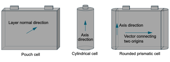
Specify the Electrode Layer Orientation (
 in Equation 16–38 in the Fluent Theory Guide).
 The following orientation types are available (see Figure 31.22: Electrode Layer Orientation):
Pouch Cell
For the Pouch Cell geometry type, you need to specify the X, Y, Z components of the Layer Normal Vector, which is the unit vector normal to the battery electrode sandwich layer surface.
Cylindrical Cell
For the Cylindrical Cell geometry type, you need to specify the X, Y, Z components of the Cylinder Axis Vector.
Rounded Prismatic Cell
For the Rounded Prismatic Cell geometry type, you need to specify the X, Y, Z components of two vectors - the Cylinder Axis Vector and the Vector Connecting Two Origins of the prismatic cell.
UDF
This option allows you to specify an electrode layer orientation for more complex battery geometry via the
DEFINE_BATTERY_SWELL_LAYER_Nuser-defined function. SeeDEFINE_BATTERY_SWELL_LAYER_Nin the Fluent Customization Manual for more information.
For steps on setting a swelling simulation, see Setting a Battery Swelling Case.
Note: Model parameters are battery specific. The default values are taken from Cai & White [90]. To simulate a battery of different design, you should provide a user-specified set of battery parameters.
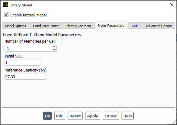
The following parameters are available under User-Defined E-Chem Model Parameters:
- Number of Memories per Cell
is the number of submodel parameters that need to be saved per computational cell during a simulation.
- Initial SOC
is the value of the battery initial state of charge.
- Reference Capacity
is the battery capacity (Ah).
In the UDF tab, you can customize various battery model parameters by hooking up your user-defined functions (UDFs).
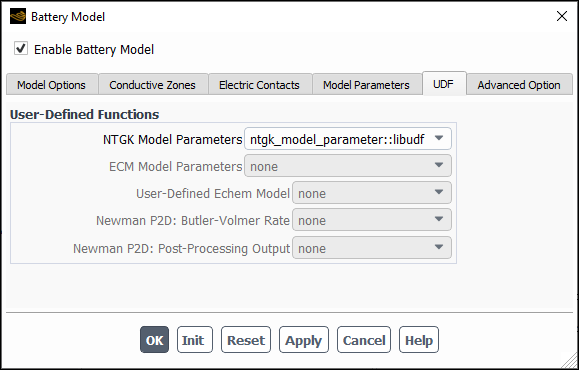
Refer to Battery Model DEFINE Macros in the Fluent Customization Manual for a list
of all available UDFs for specific battery models, their detailed descriptions and examples on
how to use them.
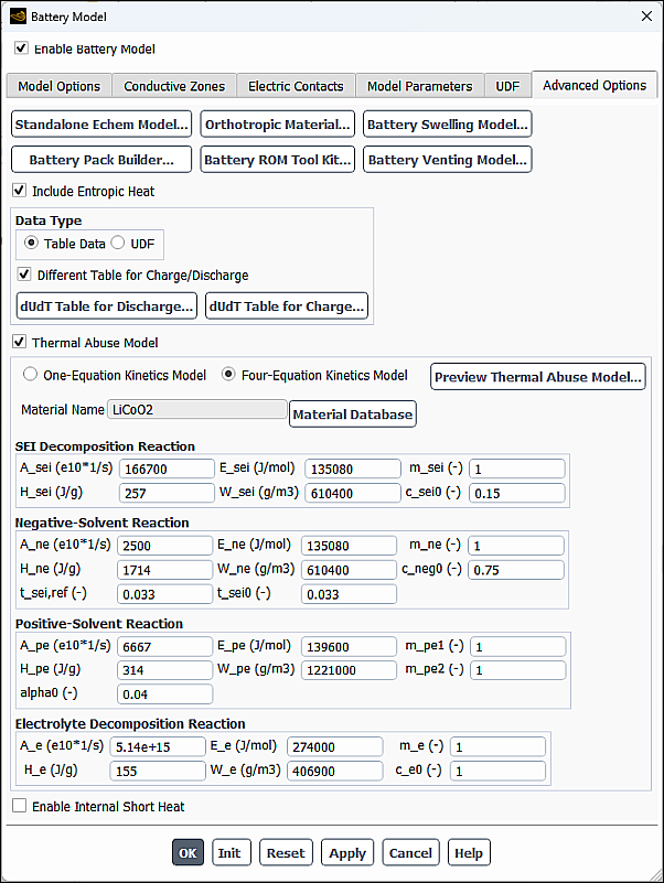
Using the Advanced Options tab of the Battery Model dialog box, you can:
Check the selected electrochemical model behavior before running the CFD case by performing a quick simulation of the electrochemical model in a standalone mode
Run the physics-based battery life model to simulate the aging process of a battery through electric load cycles in a standalone mode
Use the Battery Pack Builder tool to construct a battery pack from existing Ansys Fluent simulations of the battery module and cold plate
Create LTI-ROM or SVD-ROM training data and load SVD-ROM results into Ansys Fluent for postprocessing
Define orthotropic thermal conductivity for all battery active zones
(NTGK and ECM models only) Enable and set the empirical-based battery swelling model for an FSI coupled simulation
Enable and set the battery venting model
Include the entropic heat term in the battery thermal analysis when any of the electro-chemical submodels is used
Perform thermal abuse analysis
For additional information, see the following sections:
- 31.2.3.6.1. Running the Standalone Echem Model
- 31.2.3.6.2. Simulating the Aging Process of a Battery (Standalone Mode)
- 31.2.3.6.3. Using the Battery Pack Builder Tool
- 31.2.3.6.4. Using the Battery ROM Tool Kit
- 31.2.3.6.5. Defining Orthotropic Thermal Conductivity
- 31.2.3.6.6. Using the Empirical-Based Battery Swelling Model
- 31.2.3.6.7. Battery Venting Model
- 31.2.3.6.8. Including the Entropic Heat Effects
- 31.2.3.6.9. Using the Thermal Abuse Model
Prior to running a coupled electrochemical-thermal simulation, you should perform a quick analysis of your electrochemical model by simulating it in a standalone mode. The standalone model calculation uses the operating conditions that you have specified in the Model Options tab (such as electric load type and value) and the echem model parameters that you have defined in the Model Parameters tab. This preliminary analysis will allow you to confirm the electrochemical behavior of the selected submodel and, if necessary, adjust the model settings.
To run the echem model in a standalone mode:
Click .
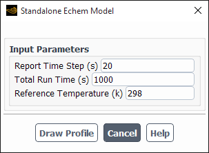
In the Standalone Echem Model dialog box that opens, specify the following parameters:
Report Time Step: The time interval at which the results will be saved and reported.
Total Run Time: The total time for running the stand-alone model simulation.
Reference Temperature: The temperature level at which you want to simulate your electrochemical model.
(Neman’s P2D model with battery swelling effects only) Mechanical Load Type: The external mechanical load that causes electrode elastic deformation (see Modeling Swelling in the E-Chem Standalone Mode in the Fluent Theory Guide for more information). You can select and specify the following load types:
External Pressure: The external normal force exerted on the battery electrode layer end,
 in Equation 19–78 in the Fluent Theory Guide. A
positive value represents compression.
in Equation 19–78 in the Fluent Theory Guide. A
positive value represents compression.Total Deformation: The percentage of the total thickness change of the battery electrode layer, the right-hand side of Equation 19–79 in the Fluent Theory Guide.
External Stiffness: The effective stiffness of external constraint applied to the battery electrode layer,
 in Equation 19–80 in the Fluent Theory Guide.
Initiate the electrochemical model simulation by clicking .
Once the calculation is complete, the Plot Profile Data dialog box opens.
Using the Plot Profile Data dialog box, visualize and analyze the results of the standalone echem model simulation. Different profiles are available for different electrochemical models.
For the NTGK model, a time history profile, called ntgk-time-history-profile, is generated after the calculation is complete. You can draw the X-Y plots of the following variables as a function of time:
soc: the battery state of charge (SOC)
voltage: the battery voltage
current: the battery electric current
power: the battery power output
For the ECM model, a time history profile, called ecm-time-history-profile, will be generated. In addition to the variables available for the NTGK model, you can also draw the X-Y plots of the following variables as a function of time:
v1:
 in Equation 19–9
v2:
 in Equation 19–9
For the Newman P2D model, the following two profiles will be generated:
Time history profile p2d-time-history-profile
Spatial field profile called p2d-field-profile
For the p2d-time-history-profile profile, you can plot the time history profile for the following variables:
current (see above)
voltage (see above)
power (see above)
ce_x=0
ce_x=lp
ce_x=lps
ce_x=lpsn
cs_x=0
cs_x=lp
cs_x=lps
cs_x=lpsn
phis_x=0
phis_x=lp
phis_x=lps
phis_x=lpsn
phie_x=0
phie_x=lp
phie_x=lps
phie_x=lpsn
where ce is the lithium-ion concentration in electrolyte phase at different locations x=0 denotes the location of the outside face of the positive electrode x=lp denotes the interface of the positive electrode and separator x=lps denotes the interface between the separator and negative-electrode x=lpsn denotes the outside face of the negative electrode cs is the lithium concentration at the surface of the active material in electrode at different locations phis is the electric potential in the electrode solid phase at different locations phie is the electric potential in the electrolyte liquid phase at different locations For the p2d-field-profile profile, you can plot the spatial profiles of the following variables at the end of the simulation:
phi_e: the electric potential in electrolyte phase
phi_s: the electric potential in electrode phase
ce: the lithium-ion concentration in electrolyte phase
cs_center: the lithium concentration in the center of the active electrode particles
cs_average: the average lithium concentration in the active electrode particles
cs_surf: the lithium concentration at the surface of the active electrode particles
Note: SI units are always used for all the variables in the X-Y plot.
In practical Newman’s P2D model simulations of battery aging through electric load cycles, the physics-based battery life model is solved on the electrode scale in the standalone mode. Further, the standalone simulation results can be included in a 3D CFD simulation to account for the battery aging effects as described in Inputs for the Newman’s P2D Model. For more information about the theory behind the physics-based battery life model, see Physics-Based Battery Life Model in the Fluent Theory Guide.
To run the physics-based battery life model in the standalone mode:
In the Model Options tab of the Battery Model dialog box, select Newman P2D Model as the E-chemistry model.
In the Solution Options group box, select Using Profile.
In the Profile Types group box, select either Time-Scheduled or Event-Scheduled and specify a profile file to define the boundary conditions of a single electric load cycle.
In the Advanced Options tab, click Run Echem Model Standalone….
In the Standalone Echem Model dialog box, select Enable Physics-Based Battery Life Model. The dialog box expands to reveal relevant model inputs in the Physics-Based Battery Life Model Parameters group box.
In addition to specifying Report Time Step and Reference Temperature (see Running the Standalone Echem Model for their definitions), specify Total Run No. of Cycle, which is the number of times the electric load profile you provided earlier is automatically looped over during the simulation.
Note: Prior to using a large number of cycles, you should run a test with a small number of cycles (for example, less than 20) as a sanity check and an estimation of computational time.
Set up the Physics-Based Battery Life Model Parameters.
In the SEI Growth Parameters group box, you can specify:
- EC Conc.
is the concentration of ethylene carbonate (EC) in the bulk electrolyte;
 in Equation 19–58 in the Fluent Theory Guide.
- EC Diff.
is the diffusivity of EC;
 in Equation 19–58 in the Fluent Theory Guide.
- SEI Dens.
is the density of solid-electrolyte-interface (SEI);
 in Equation 19–60-Equation 19–62 in the Fluent Theory Guide.
- SEI MW
is the molecular weight of SEI;
 in Equation 19–60-Equation 19–62 in the Fluent Theory Guide.
- SEI Cond.
is the ionic conductivity of SEI;
 in Equation 19–56 in the Fluent Theory Guide.
- Ref. Rate Const.
is the rate constant of SEI formation reaction;
 in Equation 19–61 in the Fluent Theory Guide.
- Trans. Coef. c.
is the cathodic charge transfer coefficient of SEI formation reaction;
 in Equation 19–56 in the Fluent Theory Guide.
- Eq. Potential
is the equilibrium potential of SEI formation reaction;
 in Equation 19–56 in the Fluent Theory Guide.
If you want to include the effects of lithium plating in your simulation, select Include Lithium Plating and then specify the following Lithium Plating Parameters:
- Li Dens.
is the density of plated lithium;
 in Equation 19–60-Equation 19–62 in the Fluent Theory Guide.
- Li MW
is the molecular weight of plated lithium;
 in Equation 19–60-Equation 19–62 in the Fluent Theory Guide.
- Ref. Curr. Dens.
is the transfer current density of lithium deposition reaction;
 in Equation 19–57 in the Fluent Theory Guide.
- Trans. Coef. c.
is the cathodic charge transfer coefficient of lithium deposition reaction;
 in Equation 19–57 in the Fluent Theory Guide.
- Eq. Potential
is the equilibrium potential of lithium deposition reaction;
 in Equation 19–57 in the Fluent Theory Guide.
- Frac. of Li forming SEI
is the fraction of deposited lithium ions that becomes SEI;
 in Equation 19–54 and Equation 19–55 in the Fluent Theory Guide.
In the Solution Controls group box, specify controls you want to use in your simulation.
Enter the Aging Speed Multiplier, which will be applied as a scaling factor to the cycle-to-cycle increment of the SEI and plated lithium concentrations after each cycle.
In the Save Aging Effects Profile per N Cycles number entry box, specify the cycle interval at which the aging effects profiles are saved.
If you want to start your simulation from an aged battery rather than from a new one, select Start from Aged Battery.
Enter the name of the file that contains the aging effects profiles in the Import Aging Effects Profile text entry field or use the Browse... button to select it. See below for more information about aging effects profile files.
Note: When you select Start from Aged Battery, you do not need to import your customized profile file each time you run a battery simulation in the standalone mode. Once imported, the aging effects profile is stored within the case file until deleted manually or overwritten by importing a profile with the same name.
From the Aging Effects Profiles drop-down list, select a profile for the simulation initial conditions.
Initiate the electrochemical model simulation by clicking Draw Profile.
Once the simulation is complete, the aging effects profiles generated in a standalone simulation will be automatically loaded into Ansys Fluent and can be visualized and analyzed using the Plot Profile Data dialog box that opens. See Running the Standalone Echem Model for more information about the Plot Profile Data dialog box.
The following variables generated by the physics-based battery life model are saved in the time-history profile called p2d-time-history-profile and in the cycle-history profile called aging-cycle-history-profile:
cs_sei_x=lps: Concentration of SEI (mol/m3)cs_li_x=lps: Concentration of plated lithium (mol/m3)r_film_x=lps: Surface resistance of the anode particle (Ohm-m2)theoretical_capacity: Theoretical capacity of the battery electrode layer (Ah/m2)
Here,
x=lpsdenotes the interface between the separator and the negative-electrode.Note: The cycle-history profile saves the battery aging variables at the end of each electric load cycle, that is, whenever the standalone simulation reaches the end of the Time-Scheduled or Event-Scheduled profile you specified in the Battery Model dialog box.
Aging Effects Profiles
The 1D spatial results of the physics-based battery life model are saved in aging effects
profiles, which are Ansys Fluent built-in format profiles (see Profiles for more information about profile files). In the standalone mode, all the generated aging
effects profiles are saved in the file called aging-field-profile.prof.
The profiles are named aging-cycle-,
where number
is the cycle number. Each profile contains the following field variables sampled
at the cycle end:number
x: Coordinate of the anode grid center (m)cs_sei: Concentration of SEI (mol/m3)cs_li: Concentration of plated lithium (mol/m3)eta_sei: Overpotential of the SEI formation reaction (V)eta_li: Overpotential of the lithium deposition reaction (V)j_sei: Current flux at the active material pore-wall due to SEI formation reaction (A/m2)j_li: Current flux at the active material pore-wall due to lithium deposition reaction (A/m2)delta_film: Surface film thickness of the anode particles (m)r_film: Surface film electric resistance of the anode particles (Ohm-m2)por_e: Electrolyte porosity (non-unit)
Apart from postprocessing, the aging effects profiles can be used in the following two scenarios:
Scenario A: The profile can be used as initial conditions in the standalone simulation when you select the Start from Aged Battery option in the Standalone Echem Model dialog box.
Scenario B: The profile can be used as model inputs of the E-chemistry submodel calculations in the CFD simulation when you select Include Aging Effects in the Model Parameters tab. In this scenario, the aging effects are included into the Newman's P2D model using the profile as a frozen-in-time snapshot. See Inputs for the Newman’s P2D Model for details.
You can also create your customized aging effects profiles based on experimental data and import them into case. A customized profile should conform to the format of the Ansys Fluent built-in profiles described in Profiles and may contain different field variables based on different scenarios:
For Scenario A, a customized profile must at least contain the following variables:
xcs_sei
For Scenario B, a customized profile must at least contain the following variables:
xc_seir_filmpor_e
The customized profile can optionally contain cs_li, which is
otherwise treated as zero.
Note: The x-coordinate of an aging effects profile (that is, the mesh point number and anode thickness) can be different from the Newman’s P2D model mesh. A mapping is automatically performed in such a case.
Many industrial applications use a battery pack in which multiple battery modules are connected in either series or parallel. Within a pack, modules are usually laid out in some repeated pattern. In addition, a cold plate may be attached to the batteries. You can use the brute force method to build the whole pack geometry and then perform a simulation of the battery pack in Ansys Fluent. However, before running the pack simulation, separate simulations of individual battery module and a cold plate are often required. The Battery Pack Builder tool allows you to construct a battery pack directly within Ansys Fluent from existing Ansys Fluent simulations of the battery module and cold plate.
Figure 31.27: Battery Pack with a Cold Plate shows an example of a battery pack where the cold plate (a) and a single module (b) have been already simulated separately in Ansys Fluent. The Battery Pack Builder constructs the pack geometry (c) within Ansys Fluent.
To use the Batter Pack Builder tool:
In the Advanced Options tab of the Battery Model dialog box, click the button to open the Pack Builder dialog box.
In the Pack Builder dialog box, specify the following information:
Battery Module Case File: The name of the Ansys Fluent case file for the module simulation.
The battery module problem setup must be complete (that is, the electric load condition, the model selection, and the battery connections are properly defined) and ready for simulation in Ansys Fluent.
Cold Plate Case File: The name of the Ansys Fluent case file for the cold plate simulation.
The problem setup must be complete. The plate geometry must be properly oriented. If the data file of the cold plate case is available, the data file will be loaded automatically.
Location information for each module.
This can be done in two different ways:
You can manually specify the Total Number of Modules in the Battery Pack and enter the location and connection information for each module in the Translation and Rotation Info of Each Module group box.
Each module position and orientation is defined with respect to the original module geometry location by the translational and rotational movements. For the module translational movement, you need to specify the translation distances in the X, Y, and Z directions (Tran_x, Tran_y, Tran_z). For the module rotation, you need to specify the rotational origin (Orgin_x, Origin_y, Origin_z), rotational axis (Axix_x, Axis_y, Axis_z), and the and rotational angle (Angle). Each module is placed in a new location, first by a rotation movement and then by a translation movement.
For the general module connection in a pack (the Series Connection option is disable), you also need to specify the connection pattern (NS and NP).
You can import a file in a text format with location information for each module by clicking the Import Module Location File... button and then using the Select File dialog box.
An example of the location file is shown below:
(
(0  0     0  0  0  0  1  0  0  0  1  1)
(0  0  0.02  0  0  0  1  0  0  0  2  1)
(0  0  0.04  0  0  0  1  0  0  0  3  1)
...
)
Each line contains 12 numbers that describe the translation distances in the X, Y, and Z directions, the coordinates of the rotation origin, the rotation axis direction, the rotational angle for each battery module, and the connection information of the module in a pack, NS and NP. The numbers can be separated by a space or tab delimiter. An extra outer parenthesis pair is needed for the convenience of file reading.
In the above example, the three modules are connected in series. If they are connected in parallel, then the last two columns will contain the following data instead of the values shown above:
... 1  1)
... 1  2)
... 1  3)
Once the location file is imported into your case, the relevant fields in the Transition and Rotation Info of Each Module group box are automatically populated. You can edit each field as appropriate for your case.
If you want to export the module location information into a separate file, click Export Module Location File....
Series Connection: Select this option if all modules are connected in series. In this case, you do not need to define the module connection data.
Click the button to construct the battery pack.
The tool loads battery modules one by one and places them in the correct location. After all modules are loaded, the tool loads the cold plate. The battery pack builder will overwrite the previously existing geometry and replace it with the combined pack geometry, which will be displayed in the graphics window once the building process is complete.
For the convenience of zone identification in the constructed battery pack, all faces and zones in the model are renamed. For any entity in a specific module, the prefix
module#(where#is the module number for the series connection and 1s1p, 1s2p, and so on for the general connection) is used, while for the cold plate, the prefixcoldplateis used.After the build operation is completed, the pack connection information is printed in the Ansys Fluent console, as in the following example:
Number of module series stages = 2; Number of modules in parallel per series stage = 3
Number of battery series stages = 8; Number of batteries in parallel per series stage = 1
In this example, the battery pack has the 2S3P module connection pattern, and each module has the 8s1p connection pattern.
Note the following:
It is your responsibility to align the modules and the cold plate correctly. You must define the location of each module properly, so that the touching faces between the battery module and cold plate are in contact in the same plane.
During the battery pack building, different modules and a cold-plate are appended to the pack sequentially. Depending on the module case size, this may take a long time to complete. To help you estimate the loading time, some timing information is printed in the console. For example:
Done with Module 6. Total elapsed time = 235.6866s, loading time for this module = 65.208097s
Done with cold-plate. Total elapsed time = 341.55449s, loading time of cold-plate = 105.86753s
Create non-conformal interfaces between the battery modules and cold plate by selecting all the pairing faces from the Non-Conformal Pairing Faces multiple-selection list and then clicking the button.
Note: If no faces are selected in the Non-Conformal Pairing Faces multiple-selection list, then all the faces in that list will be used in the search of pairing faces. This process can be expensive for a large list of faces. Therefore, selecting the pairing faces is highly recommended to speed up this process.
The tool automatically detects the touching faces, pairs them, and generates non-conformal interfaces between them. The pairing process uses the one-to-one interface creation method. All the generated non-conformal interfaces are listed in the Mesh Interfaces list.
You can display the non-conformal pairing faces or interfaces in the graphics window by selecting them from the corresponding multiple-selection lists and clicking Display Selected Faces or Display NCI Pairs, respectively.
Click to close the Pack Builder dialog box.
Prior to running the simulation in Ansys Fluent, check the model setup and do necessary adjustments. Make sure the correct solver (steady or unsteady), all appropriate models (for example, energy equation) are used, and the correct electric load condition for the pack is applied.
Run the battery pack simulation.
You can freeze the flow field if it remains unchanged (as in a liquid cooling system) in the pack simulation to speed up the calculation. In this case, you can initialize the battery model only by clicking the button in the Battery Model dialog box to start the simulation.
Note the following limitation that exist with the Battery Pack Builder tool:
The module case file that is used to build a battery pack cannot be built from the Battery Pack Builder tool.
Simulation of a battery thermal management system can be performed accurately using computational fluid dynamics (CFD). However, CFD models can be too large and too slow for a system-level transient thermal analysis. Reduced order models (ROMs), such as LTI-ROM and SVD-ROM, can be used in the system-level analysis with minimum loss of accuracy if certain conditions are satisfied.
In the LTI-ROM [70], the battery thermal problem is regarded as a system that processes a set of input signals (simply called inputs) and yields a set of output signals (simply called outputs). For a thermal problem, the inputs are the power (or the heat source), and the outputs are the temperature rise at user-specified locations or the average temperature rise across a zone. The benefit of the Linear and Time Invariant (LTI) system is that it is completely characterized by its impulse response, and the output of an arbitrary input function can be readily computed as the convolution of the input function and the system impulse response function.
A thermal system becomes an LTI system under constant flow rate, constant material properties, and linear boundary conditions. The temperature and heat flux boundary conditions are linear, and the radiation boundary condition (if present) is nonlinear. Constant density and constant properties are fairly accurate assumptions for water-cooling battery systems. For air-cooling battery systems, these assumptions can still be valid for the range of temperature variation under consideration.
For such an LTI thermal system, given an arbitrary time history of the battery heat source, the temperature evolution at a point can be obtained solely from the impulse response function at that point (that is, from the history of the temperature increase for a given unit amount of the heat source applied to the battery cell at “zero” time). The impulse response is obtained by performing a CFD calculation. In practice, instead of using an impulse function, a unit step function is applied, and the step response is monitored. The impulse response function is the time derivative of the step response function.
The LTI-ROM can calculate only cell-average temperature or temperature at a user-specified point. To obtain the temperature field, in theory, you can monitor the response function at each control volume and use the LTI-ROM for all the control volumes. However, the computational cost of such an approach would be too high, making it impractical. The dimension reduction method [12], [68] can be used for such cases to reduce the simulation time. In this method, Ansys Fluent first runs a CFD analysis to obtain the step response of the temperature distribution. Then, the singular value decomposition (SVD) is used to separate the spatial and temporal contributions of the temperature field. The dynamics of the temperature response is approximated in a largely reduced dimension space, which is formed by keeping only the first several leading singular values and their corresponding orthonormal left singular vectors. The LTI-ROM is then applied in such a reduced dimension space. Temperature at any physical space location can be obtained by a linear combination of the temperature points in the reduced subspace.
Similar to the LTI-ROM, the battery SVD-ROM tool kit in Ansys Fluent creates only the step response functions. The SVD-ROM files generated by Ansys Fluent can be used to run simulations in Ansys Twin Builder. Contact your technical engineer for detailed information and tutorials on using SVD files generated by Ansys Fluent in Ansys Twin Builder.
To use the battery ROM tool kit, click the Battery ROM Tool Kit… button in the Advanced Options tab of the Battery Model dialog box.
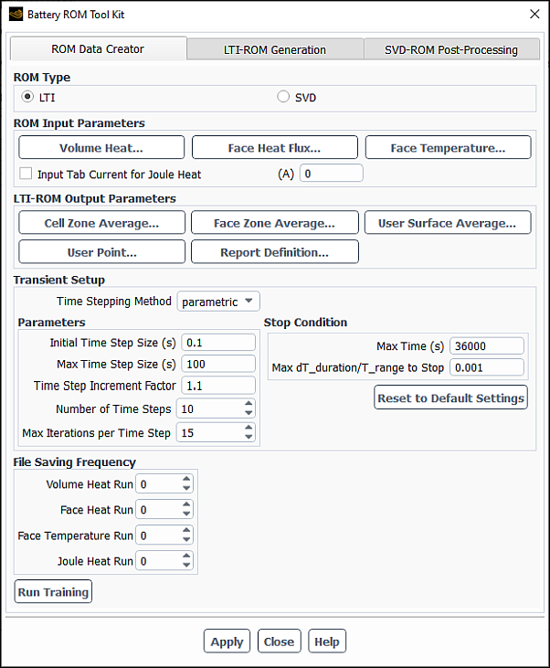
In the Battery ROM Tool Kit dialog box that opens, you can:
Create ROM training data using the ROM Data Creator tab
Compute coefficient matrices of the state space equations using the LTI-ROM Generation tab.
Do postprocessing of data obtained from the SVD-ROM tool using the SVD-ROM Post-Processing tab
In the ROM Data Creator tab (see Figure 31.29: The Battery ROM Tool Kit Dialog Box), you can create ROM training data as follows:
In the ROM Type group box, select either LTI or SVD (ROM Data Creator tab).
Wherever applicable, specify the possible heating sources using the controls in the ROM Input Parameters group box.
Define the volumetric heat in zones in the Select Volumes dialog box that opens by clicking the Volume Heat... button.
Enter a heat source value in the Value text entry box.
In the Unselected multiple-selection list, select the volume zone(s) where you want to define a volumetric source.
To define the selected zones as a single group parameter, click Add as a Group; to define the selected zones as individual parameters, click Add Individually.
The selected zones will appear in the Selected multiple-selection list. The heat source value you specified will be assigned to each individual parameter. For a single group parameter, the heat source value will be equally distributed among all the volume entities in the group.
To remove the parameter from the Selected multiple-selection list, select it and click Remove.
(group parameters only) If you want to change the heat distribution among the volume entities in the group, select that group in the Selected multiple-selection list and click Edit Group Value.... In the Value Distribution dialog box that opens, specify a source value for each zone.
In a similar manner, if necessary, define the following ROM input parameters:
Heat fluxes through a surface—in the Select Faces dialog box that opens by clicking the Face Heat Flux... button
Temperature at a surface—in the Select Faces dialog box that opens by clicking the Face Temperature... button
If you have selected Enable Joule Heat in Passive Zones in the Model Options tab, you can enable Input Tab Current for Joule Heat if you want to solve the potential equation and specify the boundary condition for the current in the text entry box.
(LTI-ROM only) Using the dialog boxes that can be accessed via the LTI-ROM Output Parameters group box, select the geometric entities of a mesh (that is, volumes, surfaces, lines, and points) and/or report definitions for which you want to obtain the following quantities after completing the training run:
average temperatures (for volumes, surfaces, and lines)
temperature at a point (for points)
temperature response for a specific variable (for report definitions)
The controls in the LTI-ROM output dialog boxes are similar to those in the ROM Input dialog boxes described above.
To select cell zones, click Cell Zone Average....
In the Select Cell Zones dialog box, select the cell zones in the same way it is done when defining ROM Input Parameters (as described above).
(group parameters only) To view the cell zones included in the group parameter, select it in the Selected multiple-selection list and click Show Group Entities.... All the cell zones will be listed in the List Entities dialog box that opens.
In a similar manner, you can select the following output entities:
Face zones—in the Select Face Zones dialog box that opens by clicking the Face Zone Average... button
User-created surfaces—in the Select Surfaces dialog box that opens by clicking the User Surface Average... button
User-created points—in the Select Point Surfaces dialog box that opens by clicking the User Point... button
Report definitions—in the Select Report-Definitions dialog box that opens by clicking the Report Definition... button
(SVD-ROM only) Select the zones for which you want to export temperature information in the Select Exported Temperature Zones dialog box that opens by clicking the Exported Temperature Zone... button (SVD-ROM Output Parameters group box).
In the Transient Setup group box, specify the parameters and the stop condition to control the time stepping during the training run:
Select either parametric (default) or file as Time Stepping Method.
If you have selected the parametric method, specify the following solution parameters and stop conditions.
In the Parameters group box, specify:
- Initial Time Step Size
is the initial time step size in the calculation.
- Max Time Step Size
is the maximum time step size.
- Time Step Increment Factor
is the factor by which the time step is increased during the solution.
- Number of Time Steps
is the number of time steps that use the same time step size.
- Max Iterations per Time-Step
is the maximum number of iterations per time step.
In the Stop Condition group box, specify:
- Max Time
is the maximum time of the transient simulation.
- Max dT_duration/T_range to Stop
is a ratio of the temperature change over the specified time duration against the temperature range. This ratio is checked for all the monitored temperatures. If they all fall bellow the specified threshold defined by this parameter, a training run stops even before the maximum time is reached.
You can use the Reset to Default Settings button to reset the parameters and stop condition to default values.
If you selected file as the Time Stepping Method, then you need to specify a filename with time stepping information or use the Browse... button to select it.
The file must contain the following three columns:
time step
number of time steps
maximum iterations per time step
Each line specifies a time marching event. The varying time step is controlled by different time marching events in the file.
An example of a file with time-stepping information is shown below:
1      5     10
1.2    5     10
3      5     10
...
10     5     10
If you want to save the simulation files during the training run (for example, for debugging purposes), you can use the below controls (in the File Saving Frequency group box) to specify the frequency with which the files should be saved for each type of input parameters.
Volume Heat Run
Face Heat Run
Face Temperature Run
Joule Heat Run (if the Input Tab Current for Joule Heat is enabled)
For example, if you have defined four volume heat input parameters and set the Volume Heat Run file saving frequency to be 1, all four simulation files will be saved after the training run. If you set Volume Heat Run to be 2, only two simulation files will be saved. By defaults, the simulation files are not saved.
Click .
The battery tool kit runs all the transient Ansys Fluent simulations sequentially for each defined ROM input parameter. The number of transient training runs equals to the total number of the ROM input parameters.
Every training simulation starts with the initial time step and runs the specified number of time steps. Then the time step is increased by the time step increment factor, and the solution runs the specified number of time steps again. This process continues until the total time reaches the specified Max Time or the stop condition is met.
After completing all solution runs, the results are saved in your work directory in a folder called LTI for the LTI-ROM or SVD for the SVD-ROM. You can then import these files into Ansys Twin Builder to run the ROM simulation. Contact your technical engineer for detailed information and tutorials on using LTI and SVD files generated by Ansys Fluent in Ansys Twin Builder. For the LTI-ROM, you can use files generated directly in the LTI-ROM Generation tool.
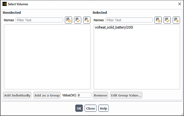
In a system simulation, an LTI-ROM model is usually solved by state space equations. Ansys Fluent provide a tool to calculate the coefficient matrices of the state space equations.
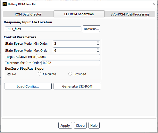
You can use the LTI-ROM Generation tab to perform the calculation as follows:
In the Response/Input File Location text entry box, specify the directory path where the response files are stored either manually or by using the button.
In the Control Parameters group box, specify the following parameters:
- State Space Model Min Order
is the minimum order of the state space model for each element. A higher order yields more accurate results, but the computation time will also increase. Note that if zero is entered, then a contribution of cross heating from other volumes may still be ignored depending on the value you specify for Tolerance for 0th Order.
- State Space Model Max Order
is the maximum order of the state space model for each element.
- Target Relative Error
is the relative error that determines the order of the state space model fitted. In general, a smaller error creates a higher order state space model.
- Tolerance for 0-th Order
allows you to ignore contributions from some inputs (for example, negligible contributions from certain cross-heating) if they are less than the specified tolerance multiplied by the largest contribution. This can significantly reduce the size of the overall model.
- NonZero StepRes Slop
is an indicator of how the end slope of the response curves is handled. You can select from the following options:
No
Calculate
Provided
For instance, in a case with all adiabatic boundary conditions, the step response will never reach a steady state condition, and the curve will have a slope. You can let the solver calculate it by selecting Calculate or provide a specific value by selecting Provided.
Click Generate LTI-ROM.
The LTI-ROM tool will use all the necessary files (including Input_PortNames.txt, Input_StepInputValues.txt, and all the response files) from the folder specified in the Response/Input File Location field, run the fitting process, and generate the matrices of the state space equation. The resulting matrices will be saved in the Thermal_ROM_Matlab.m file in the same location. This file can be used in any system simulation software that solves a state space model. The GUI settings you specified will be automatically saved in a file called Input_ROMconfig.txt, which can be read back in a later session using the Load Config... button.
Contact your technical engineer for detailed information and tutorials for the LTI-ROM generator tool.
You can use the SVD-ROM Post-Processing tab to visualize the 3D temperature field from an SVD-ROM simulation in Ansys Twin Builder:
In the SVD-ROM Post-Processing tab of the Battery ROM Took Kit dialog box, enter the name of the solution file in the One of Basis File text entry field or use the Browse... button to select it.
Enter the name of the Transient Coefficient File or use the Browse... button to select it.
You can display the reconstructed temperature field for each snapshot time and create animation from the ROM results. Contact your technical engineer for detailed information and tutorials about these functionalities.
A battery is made of a rolled or stacked sandwich structure of layered electrodes. Usually, the material properties in the in-plane direction of the electrode are different from those in the cross-plane direction. For example, the thermal conductivity in the in-plain direction is typically much larger than that in the cross-plane direction.
In battery applications, a battery module or pack may contain many batteries. In Ansys Fluent, you can define the orthotropic material for each battery in two different ways:
Define the orthotropic thermal conductivity in the Create/Edit Materials dialog box. For example, you can define the orthotropic thermal conductivity of the battery material in cylindrical coordinates as described in Cylindrical Orthotropic Thermal Conductivity. In this case, you need to create a separate solid material for each battery where each material has a unique set of the origin and cylindrical axis. This is a tedious and time-consuming process, which can lead to input errors.
Use the Ansys Fluent built-in tool that provides a fast and convenient method for defining orthotropic thermal conductivity property for each battery active zone globally.
To use the Ansys Fluent built-in tool for defining orthotropic thermal conductivity for all battery active zones:
In the Battery Model dialog box, click the button (Advanced Options tab) to open the Orthotropic Thermal Conductivity dialog box.
In the Orthotropic Thermal Conductivity dialog box, enable Use Orthotropic Thermal Conductivity for Each Battery.
The dialog box will expand to reveal the related settings.
Choose your battery cell type from the following options (see Figure 31.22: Electrode Layer Orientation):
Pouch Cell
Cylindrical Cell
Rounded Prismatic Cell
Specify the cell orientation information:
For the Pouch Cell battery type, you need to specify the X, Y, Z components of the Layer Normal Direction.
For the Cylindrical Cell battery type, you need to specify the X, Y, Z components of the Axis Vector.
For the Rounded Prismatic Cell battery type, you need to specify the X, Y, Z components of two vectors - the Axis Vector and the Vector Connecting Two Origins of the prismatic cell.
Specify the Layer Normal and Layer In-Plane components for Thermal Conductivity.
Click OK to close the Orthotropic Thermal Conductivity dialog box.
The tool will determine the origin of each battery active zone and apply the orthotropic material properties to all the active zones.
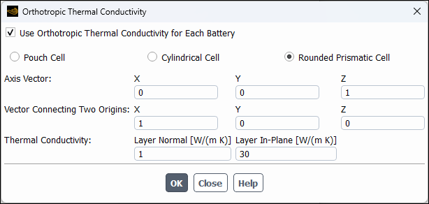
If you use the Battery Pack Builder tool, then material property settings specified in this way will be carried over to each battery module. That is, if a battery pack is constructed from a module that uses the orthotropic thermal conductivity, then the material properties specified in the Orthotropic Thermal Conductivity dialog box will be automatically applied to all batteries in all other modules. The cylindrical origin and axis of batteries in other modules will be updated automatically according to the module location and its orientation.
Note:
The orientation detection method requires each battery to have a single solid active zone. If this requirement is not met, the detected orientation may be incorrect.
If multiple batteries are used in a simulation, the orientation of all the batteries should be the same.
For the NTGK and the ECM model, the empirical-based battery model can be used in an FSI coupled simulation (see Empirical-Based Swelling Model in the Fluent Theory Guide).
To include the swelling effect, perform the following steps:
Make sure that either NTGK/DCIR Model or Equivalent Circuit Model is selected in the E-Chemistry Models group box of the Battery Model dialog box (Model Options tab).
In the Advanced Options tab, click .
In the Swelling Model Parameters dialog box that opens, enable Include Swelling Effects.
Specify the following settings:
Swell Coefficient
Neutral Swell SOC
Electrode Layer Orientation
These controls are similar to those for the Newman's P2D model. See Inputs for the Newman’s P2D Model for more information about these settings.
If you want to use your own battery swelling model, enable Customize Swelling Strain and select the name of your compiled
DEFINE_BATTERY_SWELL_STRAINuser-defined function (UDF) in the Swelling Strain UDF drop-down list. SeeDEFINE_BATTERY_SWELL_STRAINin the Fluent Customization Manual for details.
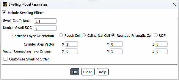
Note:
The orientation detection method requires each battery to have a single solid active zone. If this requirement is not met, the detected orientation may be incorrect.
If multiple batteries are used in a simulation, the orientation of all the batteries should be the same.
To use the Ansys Fluent battery venting model described in Battery Venting Model in the Fluent Theory Guide in your simulation, perform the following steps:
In the Advanced Options tab, click Battery Venting Model....
In the Venting Model Setup dialog box that opens, enable Venting Model.
From the Gas Release Faces selection list, select the face zones from which venting gas is released. Only faces between a battery active zone and a fluid zone are listed as potential gas release faces.
In the Options group box, you can specify the venting model options for your simulation.
For cases that do not involve the multiphase model, you can select one of the following from the Species Model drop-down list:
species-transport-w/o-reaction
eddy-dissipation-model
eddy-dissipation/finite-rate model
If the post combustion is not considered, you can choose the species-transport-w/o-reaction option. If combustion of the venting gas is important, you can choose either eddy-dissipation-model or eddy-dissipation/finite-rate model. As for the difference between these two models, refer to Volumetric Reactions in the Fluent Theory Guide for details.
For cases that involve the multiphase model, you can use the Phase of Venting Gas drop-down list to select the phase into which the venting gas is released in the multiphase simulation.
If you want to modify the venting gas composition, click Venting Gas Composition... and in the Venting Gas Composition dialog box that opens, adjust the mass fraction of each species in the venting gas mixture.
Select the Venting Gas Release Method from the following options:
Using Abuse Rate
Using File Input
If you have selected Using Abuse Rate, then you need to specify the following parameters in the Gas Release per Battery group box:
For the One-Equation Kinetics Model thermal abuse model:
Released Gas Mass: is
 in Equation 19–42 in the Fluent Theory Guide
For the Four-Equation Kinetics Model thermal abuse model:
SEI Decomposition Reaction: is
 in Equation 19–43 in the Fluent Theory Guide
Positive-Solvent Reaction: is
 in Equation 19–43 in the Fluent Theory Guide
Negative-Solvent Reaction: is
 in Equation 19–43 in the Fluent Theory Guide
Electrolyte Decomposition Reaction: is
 in Equation 19–43 in the Fluent Theory Guide
If you have selected Using File Input, then you need to specify the following:
Activation Temperature: the temperature level at which the gas venting is activated
The name of the file with the venting gas release rate information in the Specify File text entry field. Alternatively, the file can be provided using the Select File dialog box, which is opened by clicking the Browse... button. The file should contain three columns of data separated by spaces or tabs:
time in second
venting gas temperature in Kelvin
venting gas release rate in kg/s
An example of an input file is shown below:
0        400       1e-3
10       400       1e-3
10.1     450       2e-3
100      450       2e-3
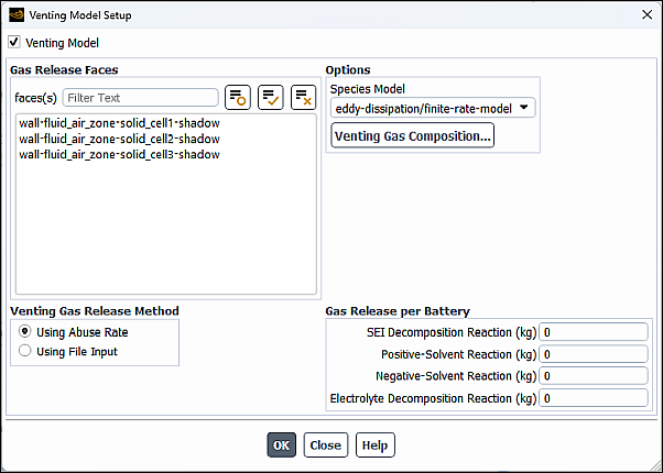
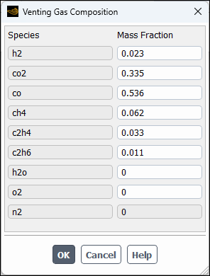
Once the solution is completed, in addition to the battery variables listed in Postprocessing the MSMD Battery Model, the following variable becomes available for postprocessing of simulations that involve the venting model (in the Battery Variables... category):
Venting Gas Mass Source
This variable can be used to display where the venting gas is added in the domain. The volume integral of Venting Gas Mass Source gives the total venting gas release rate in kg/s.
Note: The venting valve model is not implemented in the current release. For information on how to model the venting valve in a simulation, contact your support engineer at Ansys Fluent for guidance.
When any of the electrochemical submodels is used in the calculation, you can include entropic heat in the heat source calculation (Equation 19–8, Equation 19–13, and Equation 19–30 in the Fluent Theory Guide). To do so, follow the steps below.
Enable Include Entropic Heat.
In the Data Type group box, select the specification method for the
 term in the entropic heat equations (Equation 19–8, Equation 19–13, and Equation 19–30 in the Fluent Theory Guide) from the following
options:
term in the entropic heat equations (Equation 19–8, Equation 19–13, and Equation 19–30 in the Fluent Theory Guide) from the following
options:Data Table
UDF
If you have selected Data Table, click to define a lookup table for
 at different temperature and SOC levels in the dUdT Data
Table dialog box that opens.
at different temperature and SOC levels in the dUdT Data
Table dialog box that opens.The dUdT Data Table dialog box is similar to the Battery Aging Table dialog box in operation (see Setting the Life Model).
You can specify the following inputs:
Temperature Levels
Soc Levels
Values of Temperature
Values of SOC
dUdT values for each SOC-temperature pair
If you want to specify different tables for discharging and charging, do the following:
Enable Different Table for Charge/Discharge.
Click and specify data for battery discharging in the dUdT Data Table dialog box that opens.
Similarly, click and specify data for battery charging.
If you have selected UDF, you need to compile a
DEFINE_BATTERY_ENTROPIC_HEATuser-defined function and hook it using the Entropic Heat UDF dropdown list. SeeDEFINE_BATTERY_ENTROPIC_HEATin the Fluent Customization Manual for details.
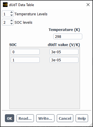
To model the thermal abuse, select the Thermal Abuse Model option. The Battery Model dialog box expands to show additional model parameters (see Figure 31.25: The Battery Model Dialog Box (Advanced Options Tab)).
You can select the following options to model thermal runaway reactions:
One-Equation Kinetics Model
Four-Equation Kinetics Model
Further details on these models are provided below.
For theoretical information about the thermal abuse model, see Thermal Abuse Model.
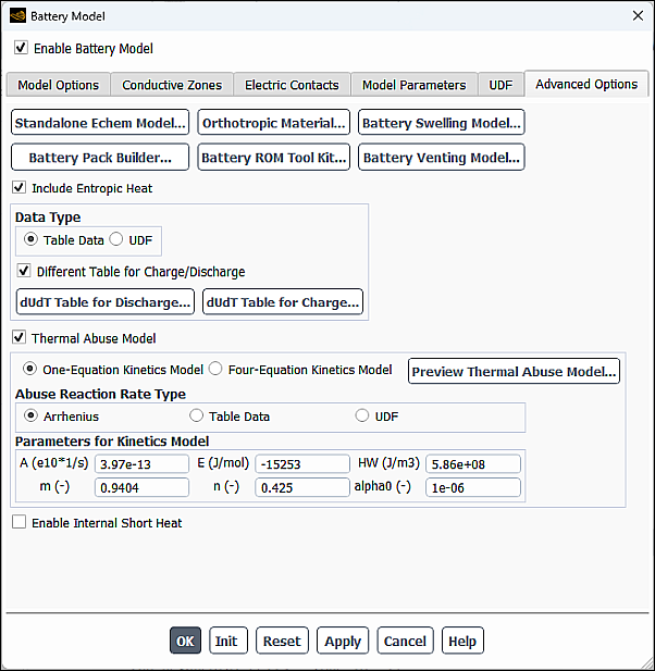
For the One-Equation Kinetics Model, you can select the Abuse Reaction Rate Type from the following options:
Arrhenius
Table Data
UDF
If you have selected Arrhenius, you need to specify the battery
constants  ,
,  ,
,  ,
,  , and
, and  used in Equation 19–33
through Equation 19–34, as well as the initial
value for
used in Equation 19–33
through Equation 19–34, as well as the initial
value for  (Parameters for Kinetics Model group box).
If you have selected Table Data, you need to specify:
Initial Reaction Progress Variable: Is the initial value of
in Equation 19–33 and
Equation 19–34.Specific Heat Release, HW: Is
in Equation 19–34.Data for the abuse reaction rate table where the temperature increase rate is defined as a function of the temperature. You need to enter the following inputs in the dialog box that opens by clicking the button:
Temperature Levels
Temperature
Rate dT/dt
The controls in the dialog box are similar to those in the Battery Aging Table dialog box described in Setting the Life Model.
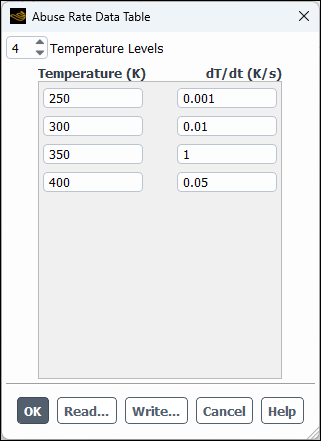
If you have selected UDF, you need to specify Initial
Reaction Progress Variable and Specific Heat Release, HW,
and select the name of your compiled DEFINE_BATTERY_ABUSE_RATE UDF
from the Abuse Reaction Rate UDF drop-down box. The UDF will be used to
compute  in Equation 19–33 and
Equation 19–34. See
in Equation 19–33 and
Equation 19–34. See
DEFINE_BATTERY_ABUSE_RATE
in the Fluent Customization Manual for details.
When you select Four-Equation Kinetics Model, you can specify the
battery constants  ,
,  ,
,  ,
,  , and
, and  used in Equation 19–35) through
Equation 19–39, as well as the initial values for
used in Equation 19–35) through
Equation 19–39, as well as the initial values for
 ,
,  ,
,  , and
, and  .
.
You can include the internal short circuit reaction (Equation 19–40 in the Fluent Theory Guide) to consider the possible initiation of an internal short circuit and its propagation in a battery by selecting the Enable Internal Short Heat option. Once this option is enabled, you need to specify the following model constants for the reaction in the Internal Short Heat Reaction group box (see Figure 31.25: The Battery Model Dialog Box (Advanced Options Tab)):
- A_ec
is a pre-exponential factor,
 in Equation 19–40 in the Fluent Theory Guide.
- E_ec
is the activation energy of the reaction,
 in Equation 19–40 in the Fluent Theory Guide.
- H_ec
is the heat of the short-circuit electrochemical reaction,
 in Equation 19–39 in the Fluent Theory Guide.
- T_trigger
is the user-specified trigger temperature,
 in Equation 19–41 in the Fluent Theory Guide.
- Soc
is the progress variable for the internal short reaction,
 in Equation 19–40 in the Fluent Theory Guide.
If you are using the Four-Equation Kinetics model, you can import kinetics data of the abuse reactions from the Ansys Fluent database using the below steps:
Click the Material Database button next to Material Name.
In the Material Database for Abuse Kinetics dialog box, select the appropriate cathode material from the Available Material List.
The reaction properties are displayed in the Properties group box.
Import kinetics data by clicking Copy.
The name of the copied material is displayed in the Material Name text box, and the kinetics data is automatically copied to the correspondent reaction group boxes in the Advanced Options tab of the Battery Model dialog box.
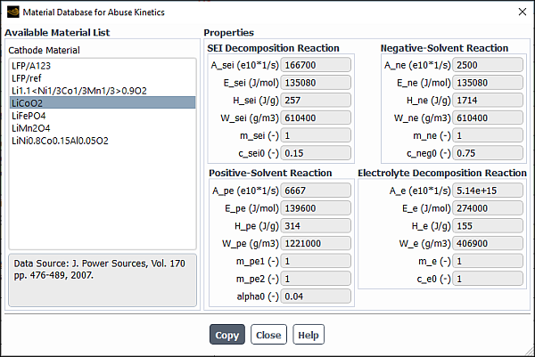
Before running a CFD simulation, you can run the standalone thermal abuse model to compute the abuse reaction behavior and display the results in the graphics windows. This tool can be used to quickly assess the abuse model you are using in your simulation. To use this tool, click the button, and in the Standalone Thermal Abuse Model dialog box that opens, specify the following parameters in the Model Inputs group box:
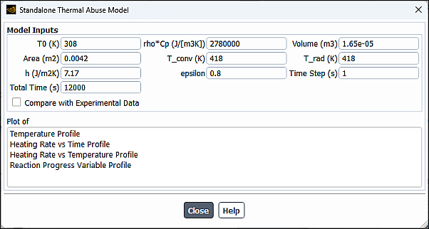
T0: Is the initial temperature
rho*Cp: Is the volumetric heat capacity
Volume: Is the battery volume
Area: Is the battery external area
T_conv: Is the environment temperature for convective heat transfer
T_rad: Is the environment temperature for radiation heat transfer
h: Is the heat transfer coefficient between battery and its surrounding environment
epsilon: Is the battery surface emissivity
Time Step: Specifies the time step size used in the calculation
Total Time: Specifies the total calculation time
If you want to compare the temperature prediction with experimental data, enable the Compare with Experimental Data option and specify the name of the ARC experimental data file in the File Name text box. Alternatively, the file can be selected using the Select File dialog box, which is opened by clicking the Browse... button.
Once you entered the model inputs, you can click one of the plots (Temperature Profile, Heating Rate vs Time Profile, Heating Rate vs Temperature Profile, or Reaction Progress Variable Profile) in the Plots of group box to display the simulation results in the graphics window. Note that the standalone solver automatically performs computations in the background once you click one of the available plots. After reviewing the results, you can adjust the rate parameter if needed.
For both One-Equation Kinetics Model and Four-Equation Kinetics Model, you can select Run Thermal Abuse Model Only (Battery Model is Turned off) if you want to solve the energy equation (Equation 19–3) alone. Otherwise, the two battery potential equations (Equation 19–4) will also be solved.
Note:
The kinetics parameters in thermal abuse models are specific to the battery material. The default settings may not be appropriate for your battery. You must provide parameter data for your own battery.
For the One-Equation thermal abuse model, you can use the Ansys Fluent parameter estimation tool available through the TUI to compute the kinetics parameters from the battery oven testing data. Once the fitting is complete, the abuse rate data are passed to the thermal abuse model in both Arrhenius and Table Data formats, and the following text entry fields are automatically populated with fitted results:
Arrhenius type: parameters in the Parameters for Kinetics Model group box (Battery Model dialog box)
Table Data type: parameters in the Abuse Rate Data Table dialog box
The experimental conditions used in the fitting are passed to the Standalone Thermal Abuse Model dialog box. You can run the standalone abuse model to evaluate the fitting quality and adjust the Arrhenius parameters or the table data to better match the experimental data.
For details, see Using Parameter Estimation Tools.
External Short-Circuit
To define the external short-circuit: In the Battery Model dialog box, under the Model Options tab, select Specified Resistance and specify a value for External Resistance. See Specifying Battery Model Options for details.
Internal Short-Circuit
The intensity of the internal short-circuit is determined by the value of volumetric
contact resistance  (External and Internal Electric Short-Circuit Treatment. In the
Ansys Fluent battery model, this value is saved in a predefined user-defined memory allocation,
Short Circuit Resistance. You can modify the value of
this user-defined memory allocation to simulate the internal short circuit.
(External and Internal Electric Short-Circuit Treatment. In the
Ansys Fluent battery model, this value is saved in a predefined user-defined memory allocation,
Short Circuit Resistance. You can modify the value of
this user-defined memory allocation to simulate the internal short circuit.
By default, the contact resistance is set to a very large number, so that  and
and  , that is, there is no internal short.
You can simulate an internal short-circuit using either of the following two ways:
Patching: Patch the contact resistance to the short circuit zone. The short circuit zone can be defined by creating a region cell register using the Region Register dialog box. See Region in the Fluent User's Guide for more details.
Using UDF: Use
DEFINE_ADJUSTorDEFINE_ON_DEMAND UDFsto specify the contact resistance using the UDM macro,C_BATTERY_SHORT_R(c,t). The contact resistance could be a function of location and time. See the Fluent Customization Manual for details.
The internal short-circuit model is available only for the MSMD solution method.
The procedure for setting up a battery simulation that involves swelling is described below. Note that only steps that are pertinent to modeling swelling are listed here. You will also need to define the other settings (such as other material properties, boundary conditions, other models) as usual. For information about inputs related to other Ansys Fluent models that you are using in your simulation, refer to the appropriate sections for those models.
In the Model Options tab of the Battery Model dialog box, make sure that either MSMD or Circuit Network is selected as the Solution Method, and Newman P2D Model, NTGK/DCIR Model, or Equivalent Circuit Model is selected as the E-chemistry Model.
Specify the battery swelling model parameters.
For NTGK or ECM battery model cases, follow the steps for including swelling effects outlined in Using the Empirical-Based Battery Swelling Model .
For Newman's P2D battery cases, specify the swelling model parameters described in Inputs for the Newman’s P2D Model.
Once the battery swelling model is enabled, the Young's modulus of the battery active zone material will be automatically set to the average of the battery swelling model's inputs for the positive electrode, negative electrode, and separator.
Setup the structure model as described in Setting Up an Intrinsic Fluid-Structure Interaction (FSI) Simulation.
The Battery Effects option will be automatically selected in the Structural Model dialog box.
Define the boundary conditions for all the battery wall zones.
See Setting Up an Intrinsic Fluid-Structure Interaction (FSI) Simulation for details.
If you want to simulate the flow around the battery module deformed due to swelling, set up the dynamic mesh model.
In the Dynamic Mesh task page, select Smoothing as Mesh Methods.
In the Mesh Method Settings dialog box (that opens by clicking ), select Linearly Elastic Solid for the smoothing method.
Create dynamic mesh zones.
In the Dynamic Mesh task page, click to open the Dynamic Mesh Zones dialog box.
For each zone where considerable deformation due to the battery swelling effects is expected, select Intrinsic FSI for Type in the Dynamic Mesh Zones dialog box.
Note:You can keep the remaining settings at their default values.
It is recommended that you create dynamic mesh zones for all fluid zone adjacent to the battery surface.
Click .
See Using Dynamic Meshes for more information.
The parameters for the NTGK, ECM, and one-equation thermal abuse models are battery specific. In theory, they can be fitted from some standard battery's testing data. Ansys Fluent provides parameter estimation tools for computing parameters for these models. The tool can be accessed from the graphical user interface (GUI) and text user interface (TUI).
For the NTGK/DCIR and ECM models, you can access the parameter estimation tool from the Battery Model dialog box as described in the following sections:
NTGK Model: Inputs for the NTGK/DCIR Model
Equivalent Circuit Model: Inputs for the Equivalent Circuit Model
To access the parameter estimation tool for the NTGK, ECM, and one-equation thermal abuse models in the text user interface (TUI), issue the following text commands:
define/models/battery-model/parameter-estimation-tool
Parameter Estimation for Model:
	1: NTGK Model
	2: ECM Model
	3: Thermal Abuse Model
Model option:  [1]
After you select a model option in the TUI, you will be prompted for information specific to the selected model.
For additional information, see the following sections:
The NTGK model parameters are fitted as functions of DOD and temperature. To fit the NTGK model parameters, you need to have battery's discharging curves at different constant C-rates. You can use testing data at different temperatures.
To use the parameter estimation tool for the NTGK model:
At the prompt, enter the testing data filenames.
The file format will be displayed in the Fluent console.
See Inputs for the NTGK/DCIR Model for an example of an input file.
Note:The input file order does not matter.
You can use basic wildcards such as "*" and "?" to specify multiple files.
Once you specified all file names, you can enter
quit(or a substring, such asq) or press Enter at the prompt to exit the file name specification loop.
For each temperature level, enter the temperature value and provide files containing testing data at the specified temperature.
After you specify input file names for different C-rate testing data, enter responses to the following prompts:
Battery capacity: Specifies capacity of the tested battery. Its value will be automatically transferred and displayed in the Reference Capacity text entry box in the Battery Model dialog box (Model Parameters tab).Number of DOD-levels: Is used in the fitting. The default value of 30 DOD levels is usually sufficient.Include capacity fade effect: Enables the capacity fade model.
If you use testing data from only one temperature level, the fitting results in both polynomial and table data types will be transferred to the Battery Model dialog box and to the parameter data table dialog boxes. In this case, the Polynomial data type will be automatically selected in the Battery Model dialog box, respectively. You can use either data type in your simulation.
The following is an example of using the parameter estimation tool for fitting the NTGK model parameters:
Parameter Estimation for Model: 1: NTGK Model 2: ECM Model 3: Thermal Abuse Model Model option: [1]1-- Make sure every input file has this format -- Crate 1.0 Temperature 300.0 time_1 voltage_1 time_2 voltage_2 ... ... ------------------------------------------------ file name for curve (wildcards "*" and "?" can be used within the file names) []ntgk-*.datThe following 15 new curves have been added: ntgk-3C-290K.dat ntgk-3C-300K.dat ntgk-2C-310K.dat ntgk-4C-300K.dat ntgk-5C-310K.dat ntgk-1C-310K.dat ntgk-4C-310K.dat ntgk-2C-290K.dat ntgk-5C-290K.dat ntgk-3C-310K.dat ntgk-1C-290K.dat ntgk-2C-300K.dat ntgk-5C-300K.dat ntgk-4C-290K.dat ntgk-1C-300K.dat file name for curve (wildcards "*" and "?" can be used within the file names) []()Battery capacity (Ah) [14.6] Number of DOD-levels [20] Include Capacity Fade Effect? [yes]no
For more information, see Inputs for the NTGK/DCIR Model.
To fit the ECM model parameters, you need to have battery's Hybrid Pulse Power Characterization (HPPC) testing data at different SOC levels. Similar to the NTGK model, you can use testing data at different temperatures.
To use the parameter estimation tool for the ECM model:
At the prompt, specify the HPPC testing data file names.
For each SOC level, you must provide a separate file with battery's testing data points in text format. At least one valid SOC level testing data is required per temperature level. For good simulation results, the range of SOC levels used in the testing should cover the SOC range simulated in the CFD runs.
The file format will be displayed in the Fluent console.
See Inputs for the Equivalent Circuit Model for an example of an input file.
Note:The input file order does not matter.
You can use basic wildcards such as "*" and "?" to specify multiple files.
Once you specified all file names, you can enter
quit(or a substring, such asq) or press Enter at the prompt to exit the file name specification loop.
After you specify input file names, enter responses to the following prompts:
Battery capacity: Specifies capacity of the tested battery. Its value will be automatically transferred and displayed in the Reference Capacity text entry box in the Battery Model dialog box (Model Parameters tab).Circuit Model:Enter
1if you want to use the 4P parameter model (one RC loop circuit)Enter
2if you want to use the 6P parameter model (two RC loop circuit).
Fitting Method:Enter
1if you want to use the JH methodThe JH method uses HPPC testing data only from the relaxation period.
Enter
2if you want to use the LM method.The LM method uses data from both pulse and relaxation periods.
Although the parameter estimation tool does not require the testing battery's capacity, you must specify this value.
Specify whether the capacity fade effect is considered or not. If your answer is
yes, you also need to specify a set of testing data files for discharging curves at different discharging rates (as for the NTGK fitting process).
If you provide testing data files at different temperatures, the parameter estimation tool will perform the fitting for each temperature level. Ansys Fluent will report the fitted results in the console and automatically pass them in a table data type to the parameter data table dialog boxes. The Table data type will be automatically selected in the Battery Model dialog box (Model Parameters tab). This will allow you to consider the temperature-dependent effect.
The following is an example of using the parameter estimation tool for fitting the ECM model parameters.
Parameter Estimation for Model: 1: NTGK Model 2: ECM Model 3: Thermal Abuse Model Model option: [2]2-- Make sure every input file has this format -- SOC 0.6 I 3.153 Temperature 300.0 time_1 voltage_1 time_2 voltage_2 ... ... ------------------------------------------------ where SOC: soc level I: pulse current file name for curve (wildcards "*" and "?" can be used within the file names) []soc??-???k.datThe following 30 new curves have been added: soc02-310k.dat soc09-290k.dat soc10-290k.dat soc05-290k.dat soc02-290k.dat soc06-300k.dat soc01-290k.dat soc05-300k.dat soc02-300k.dat soc08-300k.dat soc03-310k.dat soc05-310k.dat soc03-290k.dat soc04-290k.dat soc10-310k.dat soc03-300k.dat soc07-310k.dat soc04-310k.dat soc08-290k.dat soc09-310k.dat soc01-300k.dat soc10-300k.dat soc01-310k.dat soc07-300k.dat soc06-290k.dat soc06-310k.dat soc04-300k.dat soc08-310k.dat soc07-290k.dat soc09-300k.dat file name for curve (wildcards "*" and "?" can be used within the file names) [] () Battery capacity (Ah) [14.6] Circuit Model: 1: 4P parameter model (one RC loop) 2: 6P parameter model (two RC loops) Circuit model option: [2] Fitting Method: 1: Jiang-Hu Method (JH) 2: Levenberg-Marquardt Method (LM) Fitting method option: [2] Include Capacity Fade Effect? [yes]no
For more information, see Inputs for the Equivalent Circuit Model.
Kinetics data used in the thermal abuse model are battery specific. Reaction kinetics parameters in Equation 19–33 can be fitted by using testing data (for example, Oven test or ARC). Temperature vs. time data collected from experiment for a battery cell under thermal abuse condition can be used as input in the parameter estimation tool.
The following thermal balance equation is used to describe the heating process and in the kinetics parameter fitting of the temperature-time data:
 | (31–1) |
| where: | |
 = volume = volume | |
 = external area = external area | |
 = material density = material density | |
 = specific heat = specific heat | |
 = heat transfer coefficient = heat transfer coefficient | |
 = Stefan-Boltzmann constant = Stefan-Boltzmann constant | |
 = surface emissivity = surface emissivity | |
 = heat of reaction = heat of reaction | |
 = pre-exponential factor = pre-exponential factor | |
 = activation energy = activation energy | |
 = reaction progress variable = reaction progress variable | |
 = temperature = temperature | |
 = ambient temperature = ambient temperature | |
 = enclosure temperature for radiation = enclosure temperature for radiation | |
 and and  = reaction order parameters = reaction order parameters |
The equation will be printed in the console for your reference.
You will be prompted to specify file names for temperature testing data and values for the variables used in Equation 31–1. For good fitting results, it is recommended that you use multiple sets of testing data obtained under different heating conditions, such as different oven temperature or different battery initial temperature.
After running the parameter estimation tool for the one-equation thermal abuse model, Ansys Fluent will obtain and pass the following parameter to the Battery Model dialog box (Advanced Options tab): A, E, HW, m, and n. These parameters will also be printed in the console.
There are two ways to initialize the battery model:
Initialize the flow field from the Solution Initialization task page. The battery model will be initialized also.
Initialize the battery model in isolation by clicking the Init button in the Battery Model dialog box. Other flow variables remain untouched.
Use the second method if you want to freeze the flow field and use a different battery model to simulate the battery field. When switching from one battery submodel to another, the battery model must be re-initialized. The Init button in the Battery Model dialog box provides a convenient way to accomplish this if you do not want to initialize the flow field.
When using the MSMD battery models in Ansys Fluent, you must define the electrical conductivity of the cell, tab, and busbar materials.
For active zone materials, you usually need to use the defined-per-uds
method, specifying different values of electrical conductivity  and
and  for the positive and negative electrodes, respectively. For passive zone
materials, usually you can use the constant method to define electrical
conductivity.
for the positive and negative electrodes, respectively. For passive zone
materials, usually you can use the constant method to define electrical
conductivity.
When you use the battery models, two potential equations are solved in addition to other fluid dynamic equations, depending on the type of simulation. The two potential equations (Potential Phi+ and Potential Phi-) are listed in the Equations dialog box, where they can be enabled/disabled during the solution process.
![]() Solution →
Solution → ![]() Controls → Equations...
Controls → Equations...
Also, if required, define advanced settings the Advanced Solution Controls dialog box.
![]() Setup →
Setup → ![]() Controls → Advanced...
Controls → Advanced...
In battery applications, battery terminal voltage, terminal current and maximum temperature of battery zones are always of great interest. To assist you in reporting solution data during battery model simulations, the following report definitions are automatically created in Ansys Fluent:
battery-max-temperature
battery-terminal-voltage (Circuit Network and MSMD solution methods only)
battery-terminal-current (Circuit Network and MSMD solution methods only)
You can use these predefined report definitions to create report files and report plots as described in Creating Report Files and Creating Report Plots.
Note that these report definitions are not available for export of copying.
You can perform postprocessing using standard Ansys Fluent quantities and variables related to the battery model under the Battery Variables... category. When using the battery model, the following additional variables will be available for postprocessing:
For the CHT Coupling and FMU-CHT Coupling solution methods:
Potential Field
Current Magnitude
Electrical Conductivity
Total Heat Source
X Current Density in Battery
Y Current Density in Battery
Z Current Density in Battery
Total Heat Source is always available. The other variables are available only if the Enable Joule Heat in Passive Zones option is selected in the Model Option tab.
For the Circuit Network solution method:
Potential Field
Current Magnitude
Electrical Conductivity
Network Current
Network Voltage
Network State of Charge
Total Heat Source
X Current Density in Battery
Y Current Density in Battery
Z Current Density in Battery
Network Current, Network Voltage, Network State of Charge, and Total Heat Source are always available, while the other variables are available only if the Enable Joule Heat in Passive Zones option is selected in the Model Options tab.
For the MSMD solution method:
Cathode Potential
Cell Cluster ID
Cell Voltage
Current Magnitude
Cathode Electric Conductivity
Anode Electrical Conductivity
Passive Zone Electrical Conductivity
Passive Zone Potential
State of Charge
Joule Heat Source
Echem Heat Source
Entropic Heat Source
Short-Circuit Heat Source
Total Heat Source
Short Current Source
Echem Current Source
Total Current Source
Short-Circuit Resistance
X Current Density for phi+
Y Current Density for phi+
Z Current Density for phi+
X Current Density for phi-
Y Current Density for phi-
Z Current Density for phi-
X Current Density in Battery
Y Current Density in Battery
Z Current Density in Battery
Newman P2D: Average ce in Cathode (Newman's P2D model only)
Newman P2D: Average ce in Separator (Newman's P2D model only)
Newman P2D: Average ce in Anode (Newman's P2D model only)
Newman P2D: Average cs in Cathode (Newman's P2D model only)
Newman P2D: Average cs in Anode (Newman's P2D model only)
Newman P2D: Average phis in Cathode (Newman's P2D model only)
Newman P2D: Average phis in Anode (Newman's P2D model only)
Newman P2D: Average phis in electrolyte (Newman's P2D model only)
Newman P2D: Average phi_s-phi_e at anode-separator interface (Newman's P2D model)
Li-Insertion-Induced Electrode Layer Thickness Change Ratio (
 in Equation 19–77 in the Fluent Theory Guide;
Newman's P2D model only)
in Equation 19–77 in the Fluent Theory Guide;
Newman's P2D model only)X Component of Battery Layer Normal Vector (Newman's P2D model only)
Y Component of Battery Layer Normal Vector (Newman's P2D model only)
Z Component of Battery Layer Normal Vector (Newman's P2D model only)
Total Electrode Layer Thickness Change Ratio (left-hand side of Equation 19–79 or Equation 19–80 in the Fluent Theory Guide; Newman's P2D model only)
Projected Stress in Electrode Layer Normal Direction (Newman's P2D model only)
In any of the solution methods, if the thermal abuse model is used, the following variables are also available for postprocessing:
For the one-equation thermal abuse model:
Thermal-Abuse Heat Source
Abuse: alpha
For the four-equation thermal abuse model:
Thermal-Abuse Heat Source
Abuse: Csei
Abuse: Cpe
Abuse: Cne
Abuse: Ce
Thermal-Abuse Heat Source: SEI Decomposition
Thermal-Abuse Heat Source: Negative-Solvent
Thermal-Abuse Heat Source: Positive-Solvent
Thermal-Abuse Heat Source: Electrolyte Decomposition
Thermal-Abuse Heat Source: Internal Short (with the Enable Internal Short Option only)
In addition, you can generate vector plots of the following postprocessing variables:
current-density-jp: Is the electric current vector for the potential field on the positive electrode. It is available only for the MSMD solution method.
current-density-jn: Is the electric current vector for the potential field on the negative electrode. It is available only for the MSMD solution method.
current-density-j: Is the electric current vector in the battery conductive zones. It is available if at least one potential equation is solved.
layer-nornal-direction: Is the vector of battery layer normal direction. It is only available when either the battery swelling model or the orthotropic thermal conductivity model is used where the battery layer orientation information is needed.
Note: For reviewing simulation results in CFD Post for cases involving UDS, export the solution data as CFD-Post-compatible file (.cdat) in Fluent and then load this file into CFD-Post. This will ensure that the full variable set is available for post processing in CFD-Post.