


You can include a discrete phase in your Ansys Fluent model by defining the initial position, velocity, size, and temperature of individual particles. These initial conditions, along with your inputs defining the physical properties of the discrete phase, are used to initiate trajectory and heat/mass transfer calculations. The trajectory and heat/mass transfer calculations are based on the force balance on the particle and on the convective/radiative heat and mass transfer from the particle, using the local continuous phase conditions as the particle moves through the flow. The predicted trajectories and the associated heat and mass transfer can be viewed graphically and/or alphanumerically.
The procedure for setting up and solving a problem involving a discrete phase is outlined below, and described in detail in Options for Interaction with the Continuous Phase – Postprocessing for the Discrete Phase. Only the steps related specifically to discrete phase modeling are shown here. For information about inputs related to other models that you are using in conjunction with the discrete phase models, see the appropriate sections for those models.
Enable any of the discrete phase modeling options, if relevant, as described in Options for Interaction with the Continuous Phase.
Choose a transient or steady treatment of particles as described in Steady/Transient Treatment of Particles.
Specify tracking parameters as described in Tracking Settings for the Discrete Phase Model.
Enable the required physical submodels for the discrete phase model, as described in Physical Models for the Discrete Phase Model.
Set the numerics parameters and solve the problem, as described in Numerics of the Discrete Phase Model and Solution Strategies for the Discrete Phase.
Specify the injection-specific models, initial conditions, and particle size distributions as described in Setting Initial Conditions for the Discrete Phase.
Define the boundary conditions, as described in Setting Boundary Conditions for the Discrete Phase.
Define the material properties, as described in Setting Material Properties for the Discrete Phase.
Initialize the flow field.
Solve the coupled or uncoupled flow (Solution Strategies for the Discrete Phase).
For transient cases, advance the solution in time by taking the desired number of time steps. Particle positions will be updated as the solution advances in time. If you are solving an uncoupled flow, the particle position will be updated at the end of each time step. For a coupled calculation, the positions are iterated on or within each time step.
Examine the results, as described in Postprocessing for the Discrete Phase.
If the discrete phase interacts (that is, exchanges mass, momentum, and/or energy) with the continuous phase, you should enable Interaction with Continuous Phase.
![]() Setup → Models → Discrete Phase
Setup → Models → Discrete Phase![]() Continuous Phase Interaction → On
Continuous Phase Interaction → On
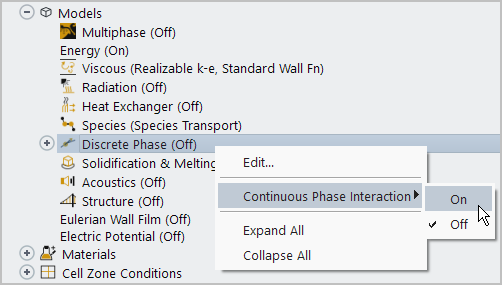
An input for the DPM Iteration Interval will appear, which allows you to control the frequency at which the particles are tracked. The DPM source terms are computed at every DPM Iterations. The DPM sources applied to the flow equations remain constant between two DPM Iterations. The amount of source considered by the solver is controlled by the under-relaxation factor specified in the Solution Control task page (see Under-Relaxation of the Interphase Exchange Terms).
For steady-state simulations, increasing the DPM Iteration Interval will increase stability but might require more iterations to converge.
The additional option Update DPM Sources Every Flow Iteration allows you to control how DPM sources are applied to the continuous phase equations. When this option is enabled, the sources are successively updated in the flow equations at every flow solver iteration according to Equation 12–512 through Equation 12–514 in the Fluent Theory Guide without repeated tracking of the particles. For unsteady simulations, this option is default and recommended. Given that the flow solver uses sufficient iterations per time step (see Under-Relaxation of the Interphase Exchange Terms), the option ensures that the complete DPM sources are consumed within a time step.
Note: When the Update DPM Sources Every Flow Iteration option is enabled, the value reported for DPM source terms (Discrete Phase Sources... category) contains the full source term.
The Discrete Phase Model uses a Lagrangian approach to derive the equations for the underlying physics, which are solved transiently. Transient numerical procedures in the Discrete Phase Model can be applied to resolve steady flow simulations as well as transient flows.
In the Discrete Phase Model Dialog Box you have the option of choosing whether you want to treat the particles in an unsteady or a steady fashion. This option can be chosen independent of the settings for the solver. Thus, you can perform steady-state trajectory simulations even when selecting a transient solver for numerical reasons. You can also specify unsteady particle tracking when solving the steady continuous phase equations. This can be used to improve numerical stability for very large particle source terms or simply for postprocessing purposes. Whenever you enable a breakup or collision model to simulate sprays, the Unsteady Particle Tracking will be switched on automatically.
When Unsteady Particle Tracking is enabled, several new options appear. If steady-state equations are solved for the continuous phase, you simply enter the Particle Time Step Size and the Number of Time Steps, thus tracking particles every time a DPM iteration is conducted. When you increase the Number of Time Steps, the droplets penetrate the domain faster.
When solving unsteady equations for the continuous phase, you must decide whether you want to use Fluid Flow Time Step to inject the particles, or you prefer a Particle Time Step Size independent of the Fluid Flow Time Step. With the latter option, you can use the Discrete Phase Model in combination with changes in the time step for the continuous equations, as it is done when using adaptive flow time stepping.
If you do not use Fluid Flow Time Step, you must decide when to inject the particles for a new time step. You can either Inject Particles at Particle Time Step or at the Fluid Flow Time Step. In any case, the particles will always be tracked in such a way that they coincide with the flow time of the continuous flow solver, as long as the maximum number of time steps used to compute a single trajectory is sufficient (see Tracking Settings for the Discrete Phase Model for details).
You can use a user-defined function (DEFINE_DPM_TIMESTEP) to change
the time step size for DPM particle tracking. The time step size can be prescribed for special
applications where a certain time step size is needed. For more information about changing the
time step size for DPM particle tracking, see DEFINE_DPM_TIMESTEP in the Fluent Customization Manual.
Important: When the density-based solver is used with the explicit unsteady formulation, the particles are advanced once per time step and are calculated at the start of the time step (before the flow is updated).
Additional inputs are required for each injection in the Set Injection Properties Dialog Box, as detailed in Defining Injection Properties. For Unsteady
Particle Tracking, the injection Start Time and Stop Time must be specified under Point Properties. Injections with start and stop times
set to zero will be injected only at the start of the calculation
( ). If the In-Cylinder mesh motion
is enabled, the start and stop times are replaced by Start
Crank Angle and Stop Crank Angle,
respectively. The injection specified in this way will be repeated
at the starting and stopping crank angle if the simulation is run
through more than one cycle. Changing injection settings during a
transient simulation will not affect particles currently released
in the domain. At any point during a simulation, you can clear particles
that are currently in the domain by clicking the button in the Discrete Phase Model Dialog Box.
). If the In-Cylinder mesh motion
is enabled, the start and stop times are replaced by Start
Crank Angle and Stop Crank Angle,
respectively. The injection specified in this way will be repeated
at the starting and stopping crank angle if the simulation is run
through more than one cycle. Changing injection settings during a
transient simulation will not affect particles currently released
in the domain. At any point during a simulation, you can clear particles
that are currently in the domain by clicking the button in the Discrete Phase Model Dialog Box.
You can choose the Parcel Release Method to determine how Ansys Fluent creates parcels. For an overview of the concept of parcels, see Parcels. The methods available are:
- standard
injects a single parcel per injection stream per time step. The number of particles in the parcel,
 , is determined as
follows:
, is determined as
follows:
(24–1)
where,  is the number of particles in a parcel
 is the mass flow rate of the particle stream
 is the time step size
 is the particle mass
This is the default method.
- constant-number
injects parcels with a user-specified number of particles per parcel. The number of parcels is determined to satisfy the specified mass-flow rate and particle size distribution for the injection.
- constant-mass
injects parcels with a user-specified parcel mass. The number of parcels is determined to satisfy the specified mass-flow rate and particle size distribution for the injection.
- constant-diameter
injects parcels with a user-specified parcel diameter. The number of parcels is determined to satisfy the specified mass-flow rate and particle size distribution for the injection.
Note that for atomizer injections, file injections, or injections that use the DEFINE_DPM_INJECTION_INIT user defined function, the Fluent solver automatically uses the default standard parcel release method. Other parcel release methods are not available.
For cases involving sprays and particle size distributions in general, the recommended setting for Parcel Release Method is constant-number. For DEM simulations, you can use constant-diameter or constant-mass to ensure that the parcel diameter does not exceed the size of the smallest cells in the computational mesh.
Note that a lower value specified for constant-number, constant-mass, or constant-diameter will result in a larger number of parcels injected and a finer discretization of the DPM phase. This may be beneficial for accuracy and stability of the calculation, at the expense of additional computational cost.
The Parcel Release Method is specified in the Parcel tab of the Set Injection Properties dialog box.
You can also choose one of several methods to control when the particles are tracked.
In steady-state simulations, particles are tracked at the user-specified intervals (DPM Iteration Interval). Individual particles are tracked from their injection position until either they escape the domain or certain termination criteria are met. Particle tracking is performed only if the global Number of Iterations is equal to or exceeds DPM Iteration Interval. The particle sources are updated during tracking, and then applied to the gas phase in subsequent flow iterations.
In transient flow simulations, particle tracking always occurs at the beginning of each flow time step, irrespective of DPM Iteration Interval. The particles are advanced in time based on the current continuous-phase solution, and DPM sources are updated. The DPM sources prevail up to the next time the particle tracker is run.
(transient flow) If the DPM Iteration Interval is larger than or equal to Max Iterations/Time Step, then particles are tracked only once per time step. If the DPM Iteration Interval is less than Max Iterations/Time Step, then the particle tracker is run multiple times during the time step. Each time the particle tracker is used, particles are returned to their original state at the beginning of the time step. Then particles are advanced in time based on the current continuous-phase solution, and DPM sources are updated. If Particle Time Step is larger than Fluid Flow Time Step (to allow injection of particles at a different time scale than the fluid), then particles are advanced only for the fluid flow time step.
(transient flow) If you specify a value of zero as the DPM Iteration Interval, the particles are advanced at the end of the time step. Note that if you have previously enabled the resetting of DPM source terms at the beginning of every time step using the TUI command
define/models/dpm/interaction/reset-sources-at-timestep?, Ansys Fluent will disable this option once you set the DPM Iteration Interval to zero, because this feature combination is not advisable.
In cases where Interaction with Continuous Phase is enabled, you must provide a sufficient number of particle source term updates to ensure that particle source terms reach their final values (see Figure 24.58: Effect of Number of Source Term Updates on Source Term Applied to Flow Equations). This can be achieved either by setting the DPM under-relaxation factor to 1 or in other cases by enabling Update DPM Sources Every Flow Iteration. If the latter is disabled and the DPM under-relaxation factor is less than 1, then the value you specify for DPM Iteration Interval must be small compared to Max Iterations/Time Step.
Important:
In steady-state discrete phase modeling, particles do not interact with each other and are tracked one at a time in the domain.
If the collision model is used, you will not be able to set the DPM Iteration Interval. Refer to Collision and Droplet Coalescence Model Theory in the Fluent Theory Guide for details about this limitation.
Note: As explained in Setting Initial Conditions for the Discrete Phase, the injection flow rate is defined per unit meter of depth in
2D problems. In such cases, each injected parcel is considered to
be a solid cylinder of diameter  and depth 1 meter. The parcel volume is then expressed
as:
and depth 1 meter. The parcel volume is then expressed
as:

However, the particles that are dense-packed in the parcel are assumed to be spheres rather than pucks (ice-hockey). The volume of each particle is the same as in 3D cases:

Consider next the theoretical atomic packing factor  of spherical particles
in a cylinder of one meter depth, also expressed as the volume ratio
of all particles to all injected parcels.
of spherical particles
in a cylinder of one meter depth, also expressed as the volume ratio
of all particles to all injected parcels.
In 2D, the particles of diameter  are
stacked on top of one another in a cylinder of diameter
are
stacked on top of one another in a cylinder of diameter  and depth 1 meter. The total number of particles that can be stacked
in the cylinder in such a way is
and depth 1 meter. The total number of particles that can be stacked
in the cylinder in such a way is  . The total volume occupied by
these particles is
. The total volume occupied by
these particles is

The volume of the surrounding parcel cylinder of depth 1 m is

The atomic packing factor  will have a constant value of 2/3 when
expressed as:
will have a constant value of 2/3 when
expressed as:

In order to use the same parameters (spring constant  and coefficient of restitution
  ) for the DEM spring
dashpot models in both 3D and 2D simulations, parcels of the same
mass must be injected in 3D and 2D.
) for the DEM spring
dashpot models in both 3D and 2D simulations, parcels of the same
mass must be injected in 3D and 2D.
In 3D, the injected parcel is a sphere with diameter  and mass
  . The number of spherical particles
in a spherical parcel is calculated by
. The number of spherical particles
in a spherical parcel is calculated by

In 2D, the parcel is a cylinder of 1 m depth. This cylinder
has the same mass as the spherical parcel in 3D ( ), but its
volume differs and is calculated as:
), but its
volume differs and is calculated as:

The number of particles per cylindrical parcel NP and the volume they occupy is the same as in 3D, that is

Since the ratio of these two volumes must be equal to the theoretical
atomic packing factor  , we obtain

The parcel diameter in 2D can then be calculated as:

Note that in 2D, the parcel diameter  is used as a collision range and it is
different than the parcel diameter
is used as a collision range and it is
different than the parcel diameter  in 3D.
For each parcel release method, the input values for the parcel
mass and parcel diameter ( and
and  , respectively) are the same in both 3D and 2D, while
the output values for parcel diameters are different:
, respectively) are the same in both 3D and 2D, while
the output values for parcel diameters are different:  in 2D simulations and
  in 3D simulations.
You will use two parameters to control the time integration of the particle trajectory equations:
the maximum number of time steps
This factor is used to abort trajectory calculations when the particle never exits the flow domain.
the length scale/step length factor
This factor is used to set the time step size for integration within each control volume.
Each of these parameters is set in the Discrete Phase Model Dialog Box (Figure 24.1: The Discrete Phase Model Dialog Box - Tracking Tab) under Tracking Parameters in the Tracking tab.
![]() Setup → Models
→ Discrete Phase
Setup → Models
→ Discrete Phase![]() Edit...
Edit...
For the Tracking Parameters, you can specify:
- Max. Number of Steps
is the maximum number of time steps used to compute a single particle trajectory via integration of Equation 12–1 in the Theory Guide. When the maximum number of steps is exceeded, Ansys Fluent abandons the trajectory calculation for the current particle injection and reports the trajectory fate as “incomplete”. The limit on the number of integration time steps eliminates the possibility of a particle being caught in a recirculating region of the continuous phase flow field and being tracked infinitely. The default value for this parameter is 50,000 for steady-state particle tracking and 500 for unsteady particle tracking. Note that you may easily create problems in which the default value is insufficient for completion of the trajectory calculation. In this case, when trajectories are reported as incomplete within the domain and the particles are not recirculating indefinitely, you can increase the maximum number of steps (up to a limit of
 ).
).Note: If, when opening a previous simulation with unsteady DPM particle tracking, you receive a warning reporting that a fraction of the discrete phase mass is "behind in time", you can use the reported percentage values to determine if it is a significant enough discrepancy to warrant revising the simulation to have a higher value for Max. Number of Steps.
- Length Scale
controls the integration time step size used to integrate the equations of motion for the particle. The integration time step size is computed by Ansys Fluent based on a specified length scale
 , and the velocity of the particle (
 ) and of the continuous phase (
 ):
):
(24–2)
where
 is the Length Scale that you define. As defined by
Equation 24–2,
is the Length Scale that you define. As defined by
Equation 24–2,  is proportional to the integration time step size and is equivalent to the
distance that the particle will travel before its motion equations are solved again and its
trajectory is updated. A smaller value for the Length Scale increases
the accuracy of the trajectory and heat/mass transfer calculations for the discrete
phase.
is proportional to the integration time step size and is equivalent to the
distance that the particle will travel before its motion equations are solved again and its
trajectory is updated. A smaller value for the Length Scale increases
the accuracy of the trajectory and heat/mass transfer calculations for the discrete
phase.(Note that particle positions are always computed when particles enter/leave a cell; even if you specify a very large length scale, the time step size used for integration will be such that the cell is traversed in one step.)
Length Scale will appear in the Discrete Phase Model dialog box when the Specify Length Scale option is enabled.
- Step Length Factor
also controls the time step size used to integrate the equations of motion for the particle. It differs from the Length Scale in that it allows Ansys Fluent to compute the time step size in terms of the number of time steps required for a particle to traverse a computational cell. To set this parameter instead of the Length Scale, turn off the Specify Length Scale option.
The integration time step size is computed by Ansys Fluent based on a characteristic time that is related to an estimate of the time required for the particle to traverse the current continuous phase control volume. If this estimated transit time is defined as
 , Ansys Fluent chooses a time step size
  as
as
(24–3)
where
 is the Step Length Factor. As defined by Equation 24–3,
  is inversely proportional to the integration time step size and is roughly
equivalent to the number of time steps required to traverse the current continuous phase
control volume. A larger value for the Step Length Factor decreases the
discrete phase integration time step size. The default value for the Step Length
Factor is 5. Step Length Factor will appear in the
Discrete Phase Model dialog box when the Specify Length
Scale option is off (the default setting).
is inversely proportional to the integration time step size and is roughly
equivalent to the number of time steps required to traverse the current continuous phase
control volume. A larger value for the Step Length Factor decreases the
discrete phase integration time step size. The default value for the Step Length
Factor is 5. Step Length Factor will appear in the
Discrete Phase Model dialog box when the Specify Length
Scale option is off (the default setting).
For steady-state particle tracking, one simple general rule to follow when setting the
parameters above is that if you want the particles to advance through a domain consisting of
 mesh cells into the main flow direction, the Step Length
Factor times
mesh cells into the main flow direction, the Step Length
Factor times  should be approximately equal to the Max. Number of
Steps.
should be approximately equal to the Max. Number of
Steps.
When Accuracy Control is enabled in the Numerics tab, the settings for Step Length Factor and Length Scale will be used only to estimate the time step size of the first integration step. In all subsequent integration steps, the particle integration time step size is adapted to achieve the tolerance specified in Numerics of the Discrete Phase Model.
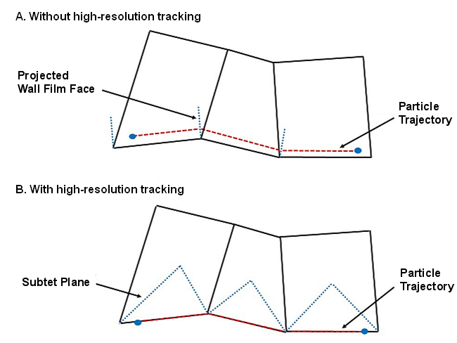
High-Resolution Tracking
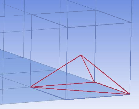
When the High-Res Tracking option is enabled in the Tracking Option group box (default), the computational cells are decomposed into tetrahedrons (subtets) and the particles tracked through the subtets. This option provides a more robust tracking algorithm and improved variable interpolation. If High-Res Tracking is not enabled, particles are tracked through the computational cells directly. Flow variables that appear in particle equations either use cell-center values or a truncated Taylor series approximation for interpolation to the particle position.
Figure 24.2: A Subtet Formed From Decomposing a Hexagonal Cell shows one of the twelve subtets produced by decomposing a hexagonal cell. In this example, the subtet is formed by the edges that connect the cell centroid and three of the eight cell nodes.
In conjunction with tracking particles through the subtets, the barycentric interpolation method is used to obtain the flow solution (such as, velocity and temperature) at the particle position. The barycentric interpolation involves linearly interpolating the flow variables from the subtet vertices to the particle position. This method provides a continuous interpolation field throughout the domain. The current interpolation method in Ansys Fluent uses the truncated Taylor series expansion, which can result in discontinuities at cell boundaries. When combined with high-resolution tracking, the barycentric interpolation provides improved accuracy and robustness and reduces the dependency on parallel partitioning. Barycentric interpolation is required for high-resolution tracking and will be enabled by Ansys Fluent automatically.
For cases with significant variations in viscosity or density (for example, cases that
involve VOF or other multiphase models) the text command options
interpolate-flow-density? and/or
interpolate-flow-viscosity? described below must be enabled to ensure
that these properties are continuous throughout the domain. Otherwise, discontinuous material
properties may result in particles being trapped at interior cell faces. Ansys Fluent automatically
enables these settings when multiphase models are enabled.
High-resolution tracking can be used with both free-stream particles and with Lagrangian wall film particles.
Note that when using high-resolution tracking, interpolation of flow gradients and temporal interpolation of the flow solution are not compatible. If both options are selected, Ansys Fluent disables the transient variable interpolation.
Once the high-resolution tracking is enabled through either the Discrete Phase Model dialog box or the text command
define/models/dpm/numerics/high-resolution-tracking/

enable-high-resolution-tracking?
Activate high-resolution-tracking? [no] yes
the below text commands become available under the
high-resolution-tracking text menu, depending on the mesh type and
solver settings.
General High Resolution Tracking Text Commands
define/models/dpm/numerics/high-resolution-tracking/check-subtet-validity?When enabled, checks the validity of a subtet when the particle first enters it. If the subtet is found to be degenerate, the tracking algorithm modifies to accommodate it. This option is useful for degeneracy in polyhedral cells shown in Figure 24.3: Degenerate Subtet in a Polyhedral Mesh. In such cases, an intersection can be missed due to a degenerate subtet. By default, this option is disabled to improve performance. It is recommended to always perform a mesh check (for example, by using the
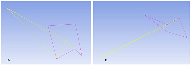
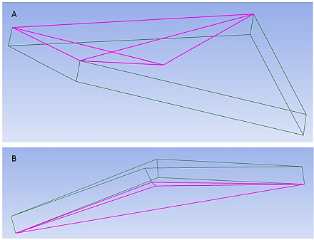
mesh/checktext command) to determine if there are degenerate subtets in the domain.An inverted subtet with negative volume can be produced when decomposing cells with highly warped faces. Figure 24.3: Degenerate Subtet in a Polyhedral Mesh and Figure 24.4: Degenerate Subtet in a Hex Mesh show examples of degenerate subtets.
In Figure 24.3: Degenerate Subtet in a Polyhedral Mesh, the left-hand side (A) illustrates a degenerate subtet (in yellow) resulting from a warped polyhedral face (in magenta). The right-hand side (B) shows the same subtet from a different angle.
In Figure 24.4: Degenerate Subtet in a Hex Mesh, the top image (A) illustrates a degenerate subtet resulting from a warped quadrilateral face of a hexagonal cell while the bottom image (B) illustrates the same subtet from a different angle.
Tracking particles through degenerate subtets can result in missed face intersections and lost particles. The degeneracy may also result in the failure of the initial location of the particle when it is first injected.
define/models/dpm/numerics/high-resolution-tracking/use-quad-face-centroid?Enables/disables using quad face centroids when creating subtets. This option changes the way hexahedral cells are decomposed to avoid creating degenerate subtets. It is useful in situations where the particle cannot be initially located in degenerate subtets formed by a warped hexahedral cell (see Figure 24.4: Degenerate Subtet in a Hex Mesh). It is recommended to always perform a mesh check (for example, by using the
mesh/checktext command) to determine if there are degenerate subtets in the domain. If degenerate subtets are found in the domain during the mesh check, Ansys Fluent automatically enables the appropriate settings (use-quad-face-centroid?and/orcheck-subtet-validity?) and displays the following message:Note: Settings to improve the robustness of pathline and particle tracking have been automatically enabled.define/models/dpm/numerics/high-resolution-tracking/project-wall-film-particles-to-film?Enables/disables projecting existing particles to Lagrangian wall film to track using high-resolution tracking.
When not using the high-resolution tracking method in Ansys Fluent, the particles are tracked slightly above the wall film surface to avoid incomplete or lost particles. When High-Res Tracking is enabled, particles are tracked directly on the surface, which improves accuracy and robustness, as shown in Figure 24.5: Lagrangian Wall Film Tracking.
When reading in a data file that contains wall film particles previously tracked without high-resolution tracking, you need to either clear the particles from the domain or project their positions to the wall film surface using the
project-wall-film-particles-to-film?text command prior to using the high-resolution tracking method. After tracking the particles for one timestep, this option can be disabled to improve performance.Note: Projecting LWF particles that have been tracked without high-resolution tracking to the film zone and continuing with high-resolution tracking sacrifices both accuracy and robustness. Therefore, removing such particles from the domain is recommended.
define/models/dpm/numerics/high-resolution-tracking/enable-automatic-intersection-tolerance?Enables/disables the automatic calculation of intersection tolerance. By default, the tolerance used in intersection calculations is scaled by the residence time of the particle in the cell to improve robustness. For most cases, the scaled tolerance is sufficient to identify all intersections of the particle trajectory and the subtet faces. You can set the intersection tolerance manually using the
set-subtet-intersection-tolerancetext command.define/models/dpm/numerics/high-resolution-tracking/set-subtet-intersection-toleranceSpecifies the tolerance used in intersection calculations. This tolerance will be scaled by the characteristic cell crossing time of the particle if the
enable-automatic-intersection-tolerance?text command is enabled. If that option is disabled, the specified tolerance will be used without scaling. The default intersection tolerance is 10-5.define/models/dpm/numerics/high-resolution-tracking/boundary-layer-tracking?Enables/disables the calculation of the particle time step size that considers both the cell aspect ratio and the particle trajectory. This method improves the accuracy of the predictions in boundary layer cells, particularly in layers where flow gradients are large.
define/models/dpm/numerics/high-resolution-tracking/enable-barycentric-intersections?Enables/disables an alternative method of calculating intersections with cell boundaries. Barycentric intersections are linear calculations and are faster than the default intersection algorithm. The default intersection algorithm is second-order for stationary meshes; therefore, using the barycentric intersection may sacrifice accuracy. You must verify that the barycentric intersections provide comparable results to the default intersection method. This option is available only for 3D stationary meshes and the double precision solver.
define/models/dpm/numerics/high-resolution-tracking/use-barycentric-sampling?When enabled, this option provides improved accuracy and parallel consistency when sampling particles at planes. This item is available only with the 3D solver. Using the double-precision solver and bounded planes is recommended.
-
define/models/dpm/numerics/high-resolution-tracking/use-particle-timestep-for-intersection-tolerance? Enables/disables the use of the particle timestep for the subtet intersection tolerance with axisymmetric grids (default: enabled). If disabled, the tolerance will be calculated in the same manner as non-axisymmetric meshes (a scaled value of the tolerance which is set using the
define/models/dpm/numerics/high-resolution-tracking/set-subtet-intersection-tolerancetext command).-
define/models/dpm/numerics/high-resolution-tracking/use-velocity-based-error-control? Enables/disables an alternative method of timestep adaption. By default, Ansys Fluent uses the half-step method of timestep adaption with particle integration. This alternative method of controlling the integration timestep based upon velocity changes is faster; however, you need to ensure that the accuracy is comparable for your specific application.
define/models/dpm/numerics/high-resolution-tracking/set-film-spreading-parameterProvides the ability to add a random component to the Lagrangian wall-film particle acceleration to reduce streaking that may result from tracking particles on faceted geometry. As small variations in face normals can produce streaks in the wall-film appearance, this parameter makes the film look smoother. The value of this parameter should range between 0 and 1.0. The default value of 0 prevents any artificial smoothing.
-
define/models/dpm/numerics/high-resolution-tracking/always-use-face-centroid-with-periodics? When enabled, Ansys Fluent uses quad face centroids when creating subtets in cases with periodic boundaries.
To avoid discontinuities in the particle forces at periodic boundaries, Ansys Fluent automatically enables the
use-quad-face-centroid?option in simulations with periodic zones. You can disable this option for cases where the particles are not crossing the periodic boundaries. This may improve performance for meshes predominantly made up of hex cells. The recommended method to ensure that degenerate subtets are still handled appropriately is to execute the following commands in this order:define/models/dpm/numerics/high-resolution-tracking/always-use-face-centroid-with-periodics?nodefine/models/dpm/numerics/high-resolution-tracking/use-quad-face-centroid?nomesh/check-
define/models/dpm/numerics/high-resolution-tracking/sliding-interface-crossover-fraction Specifies the fraction of the distance to the subtet center to move the particle.
At non-conformal interfaces, the nodes used for the barycentric interpolation are different on either side of the interface. This may result in incomplete particles due to discontinuities in the variable interpolation. The number of incomplete particles may be reduced by moving the particles slightly off of the sliding interface. Recommended values range between 0 and 0.5.
Barycentric Interpolation Method Text Commands
In addition, the following interpolation options are available under the
define/models/dpm/numerics/high-resolution-tracking/barycentric-interpolation/text menu:define/models/dpm/numerics/high-resolution-tracking/barycentric-interpolation/zero-nodal-velocity-on-walls?When enabled, sets the velocity at wall nodes to zero. (By default, the nodal velocities on walls are first reconstructed from cell and face values and then corrected to ensure that there are no velocity components directed towards the walls). This may be useful if you want to consider particle impingement on the walls. Note that enabling this option will more likely produce incomplete particles as some particles may settle on the walls.
define/models/dpm/numerics/high-resolution-tracking/barycentric-interpolation/interpolate-flow-density?Enables/disables the barycentric interpolation of the flow density. This option is recommended when the density varies with position to avoid discontinuities in the interpolated variable at cell boundaries. For constant density flows, this option is unnecessary.
define/models/dpm/numerics/high-resolution-tracking/barycentric-interpolation/interpolate-flow-viscosity?Enables/disables the barycentric interpolation of flow viscosity to the particle position. This option is recommended when the flow viscosity varies with position to avoid discontinuities in the interpolated variable at cell boundaries. For flows with constant viscosity, this option is unnecessary.
define/models/dpm/numerics/high-resolution-tracking/barycentric-interpolation/interpolate-flow-cp?Enables/disables the barycentric interpolation of specific heat to the particle position. This option is recommended when the specific heat varies with position to avoid discontinuities in the interpolated variable at cell boundaries. For flows with constant specific heat, this option is unnecessary.
define/models/dpm/numerics/high-resolution-tracking/barycentric-interpolation/interpolate-flow-solution-gradients?When enabled, flow solution gradients are interpolated to the particle position. This can be useful when using physical models that depend on these gradients (for example, the thermophoretic force, pressure-gradient force, or virtual mass force). Interpolating the gradients is highly recommended when using the trapezoidal numerics scheme, which is the default method.
define/models/dpm/numerics/high-resolution-tracking/barycentric-interpolation/interpolate-temperature?Enables/disables the barycentric interpolation of temperature to the particle position. The cell temperature is used by default in calculations of heat transfer to/from the particle.
-
define/models/dpm/numerics/high-resolution-tracking/barycentric-interpolation/interpolate-wallfilm-properties? When enabled, the wallfilm properties (film height, film mass, and wall shear) are interpolated to the particle position.
-
define/models/dpm/numerics/high-resolution-tracking/barycentric-interpolation/precompute-pdf-species? When this option is enabled for premixed or non-premixed combustion simulations, the species composition in each cell is precomputed prior to tracking particles. This approach may improve performance for cases with many particles and relatively few cells. By default, this option is set to
no, and Ansys Fluent calculates the species composition during particle tracking. The solution results will be identical for both methods.
-
define/models/dpm/numerics/high-resolution-tracking/barycentric-interpolation/user-interpolation-function Provides a hook for the
DEFINE_DPM_INTERPOLATIONuser-defined function (UDF) used to interpolate cell UDM to the particle position when using high-resolution particle tracking. SeeDEFINE_DPM_BODY_FORCEin the Fluent Customization Manual for more information about this UDF.
Particle Relocation Text Commands
The following location options are available under the
define/models/dpm/numerics/high-resolution-tracking/particle-relocation/text menu:define/models/dpm/numerics/high-resolution-tracking/particle-relocation/enhanced-cell-relocation-method?When enabled, Ansys Fluent uses a more rigorous method of locating the cell in which the particle is currently contained. This approach is computationally more expensive than the default method; however, it is recommended for cases when Fluent reports that particles are lost after the mesh has been changed due to MDM, dynamic adaption, or repartitioning.
define/models/dpm/numerics/high-resolution-tracking/particle-relocation/enhanced-wallfilm-location-method?When enabled, Ansys Fluent uses a more robust method of locating the wall film particles on the film zone after the domain has been remeshed either due to dynamic mesh movement or dynamic adaption. The improved robustness involves a performance penalty. This method is recommended for cases when Fluent reports that wall film particles are lost during relocation.
define/models/dpm/numerics/high-resolution-tracking/particle-relocation/overset-relocation-robustness-levelSets the performance/robustness trade-off when relocating particles in overset meshes. The default value is 1, which corresponds to a more robust algorithm. Performance may be improved by setting the value to 0; however, this may result in particle loss, particularly if the mesh is moving. You need to make sure that no particle loss occurs.
define/models/dpm/numerics/high-resolution-tracking/particle-relocation/use-legacy-particle-location-method?Provides the ability to use the legacy particle location method with high-resolution tracking to improve performance.
When using high-resolution tracking, the default method of locating the cells in which particles are injected is to decompose the cells into subtets and then determines if the particle is present in one of them. Dividing cells into subtets to locate the particles is more accurate and robust than the method used when high-resolution tracking is not active. However, for unsteady particle tracking in polyhedral cells, it can take considerably longer to locate the particles in the domain than with the method used when high-resolution tracking is not enabled. This option is useful when tracking in polyhedral meshes, particularly when unsteady particles that evaporate quickly are injected frequently (for example, gas turbine combustors). Note that it does not improve the particle tracking speed, only the time it takes to inject the particles.
define/models/dpm/numerics/high-resolution-tracking/particle-relocation/wallfilm-relocation-tolerance-scale-factorSets a scaling factor to modify the tolerance for locating Lagrangian wall film (LWF) particles on a film face during the relocation. The default value is 1.0. Increasing the tolerance may help when Ansys Fluent fails to locate LWF particles in such cases.
To improve accuracy and robustness, it is recommended to use the high-resolution tracking of particles from the time they are first injected. If you want to use in your simulation a data file containing particles that were tracked without the high-resolution tracking option, be aware that the cell IDs stored in the file may not be correct. If this is the case, Ansys Fluent needs to locate the cell containing the particle. For cases with many particles, cells, or parallel partitions, this may take considerable time, particularly if any of the particles are outside of the domain and cannot be located. To accelerate this process, you can enable the following text command:
define/models/dpm/numerics/high-resolution-tracking/particle-relocation/load-legacy-particles?Ensure particles are in the expected cells prior to tracking? [no]yesWhen this option is enabled, the particles that are found outside the associated cells in the Fluent data file will be moved inside these cells prior to particle tracking. Neither the mesh nor the partitioning should be modified prior to the first time the particles are tracked. If you need to perform manual or dynamic mesh adaption, you must first disable this option. This option can be enabled before or after reading the data file into Ansys Fluent.
There are eight drag laws for the particles that can be selected for each injection. These are specified on the Physical Models tab of the Set Injection Properties dialog box. See Specifying Injection-Specific Physical Models for details.
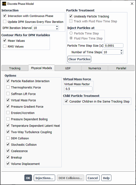
This section provides instructions for using the optional discrete phase models available in Ansys Fluent. All of them can be enabled in the Physical Models tab of the Discrete Phase Model dialog box (Figure 24.6: The Discrete Phase Model Dialog Box - Physical Models Tab).
![]() Setup → Models → Discrete Phase
Setup → Models → Discrete Phase![]() Edit...
Edit...
Further details are discussed in the following sections:
- 24.2.5.1. Including Radiation Heat Transfer Effects on the Particles
- 24.2.5.2. Including Thermophoretic Force Effects on the Particles
- 24.2.5.3. Including Saffman Lift Force Effects on the Particles
- 24.2.5.4. Including the Virtual Mass Force and Pressure Gradient Effects on Particles
- 24.2.5.5. Monitoring Erosion/Accretion of Particles at Walls
- 24.2.5.6. Pressure Options for Vaporization Models
- 24.2.5.7. Considering Pressure Dependence in Boiling
- 24.2.5.8. Including the Effect of Droplet Temperature on Latent Heat
- 24.2.5.9. Including the Effect of Particles on Turbulent Quantities
- 24.2.5.10. Including Collision and Droplet Coalescence
- 24.2.5.11. Including the DEM Collision Model
- 24.2.5.12. Including Droplet Breakup
- 24.2.5.13. Modeling Collision Using the DEM Model
- 24.2.5.14. Including the Volume Displacement of Particles
If you want to include the effect of radiation heat transfer to the particles (Equation 5–73 in the Theory Guide), you must enable the Particle Radiation Interaction option under the Physical Models tab, in the Discrete Phase Model Dialog Box (Figure 24.6: The Discrete Phase Model Dialog Box - Physical Models Tab). You also must define additional properties for the particle materials (emissivity and scattering factor), as described in Description of the Properties. This option is available only when the P-1 or discrete ordinates radiation model is used.
If you want to include the effect of the thermophoretic force on the particle trajectories (Equation 12–11 in the Theory Guide), enable the Thermophoretic Force option under the Physical Models tab, in the Discrete Phase Model Dialog Box. You also must define the thermophoretic coefficient for the particle material, as described in Description of the Properties.
For sub-micron particles, you can also model the lift due to shear (the Saffman lift force, described in Saffman’s Lift Force in the Theory Guide) in the particle trajectory. To do this, enable the Saffman Lift Force option under the Physical Models tab, in the Discrete Phase Model Dialog Box.
In cases where the density of the fluid approaches or exceeds the density of the particles (for example liquid flow with gaseous bubbles), it is recommended that you include the Virtual Mass and Pressure Gradient forces in the particle force balance. To do this, enable Virtual Mass Force and Pressure Gradient Force under the Physical Models tab in the Discrete Phase Model Dialog Box. See Other Forces in Fluent Theory Guide for information on the Virtual Mass and Pressure Gradient forces.
To monitor particle erosion and accretion rates at wall boundaries:
Enable Erosion/Accretion in the Physical Models tab of the Discrete Phase Model Dialog Box.
Enabling the Erosion/Accretion option will cause the erosion and accretion rates to be calculated at wall boundary faces when particle tracks are updated.
For each wall zone, select erosion models and specify erosion model parameters as described in Setting Particle Erosion and Accretion Parameters.
If you want to couple particle erosion with dynamic meshes to account for changes in the shape and position of eroded walls, follow the procedure described in Particle Erosion Coupled with Dynamic Meshes.
Note: The computation of the erosion rate is based on the real wall position, and for cases that involve the DPM rough wall model, variations of the wall orientation are not considered.
You can use the text interface command
define/models/dpm/options/use-absolute-pressure-for-vaporization?
to select whether the absolute pressure or a constant Operating Pressure (set in the Operating Conditions dialog box) is used in the vaporization rate calculations.
The default and recommended setting is to use the absolute pressure. However, in some incompressible flow cases, when there are large pressure variations in the droplet injection region, selecting the constant operating pressure may stabilize the solution.
See Operating Pressure, Gauge Pressure, and Absolute Pressure and Equation 8–74 for definitions of the operating pressure and absolute pressure.
If the pressure in your simulation differs from atmospheric, you should either modify the boiling point to be consistent with the average pressure in the region where the droplets evaporate, or enable the option to change the condition for switching from droplet vaporization (Law 2) to boiling (Law 3). If you modify the boiling point for the droplet material, you should also modify the latent heat value accordingly.
By default Ansys Fluent will switch from the vaporization to the boiling law when the particle
temperature has reached the boiling point defined for the droplet material (Equation 12–99 in the Theory Guide). When the Pressure Dependent
Boiling option is enabled, the switching condition will change to  , where
  is the saturation vapor pressure at the droplet temperature and
 is the domain pressure. If
  while in the boiling law, the model will switch back to the vaporization law.
If this option is enabled it is essential to enter the appropriate droplet saturation vapor
pressure data to cover the complete pressure/temperature range in your model.
while in the boiling law, the model will switch back to the vaporization law.
If this option is enabled it is essential to enter the appropriate droplet saturation vapor
pressure data to cover the complete pressure/temperature range in your model.
When Pressure Dependent Boiling is enabled, then the Temperature Dependent Latent Heat model automatically applies (see Including the Effect of Droplet Temperature on Latent Heat).
Setting the Pressure Dependent Boiling option has no effect on the multicomponent particles, where switching from the vaporization to the boiling regime is always based on the component saturation vapor pressures (see Multicomponent Particle Definition (Law 7) in the Theory Guide).
In the supercritical pressure regime, failure of the saturation temperature calculation algorithm may indicate that the multicomponent droplet has approached the critical temperature, provided that you have entered accurate vapor pressure data for all components. In such a case, you can use the following text command:
define/models/dpm/options/treat-multicomponent-saturation-temperature-failure?
Dump multicomponent particle mass if the saturation temperature calculation
      fails? [no]
y
When this option is enabled, Ansys Fluent dumps the particle mass into the continuous phase if the saturation temperature calculation fails.
Finally, selection of the Pressure Dependent Boiling option is not available with the real-gas models, as the pressure dependence always applies. See Using the Cubic Equation of State Models with the Lagrangian Dispersed Phase Models for more information.
For pressures higher than the critical pressure of the droplet material ( ), a boiling point
  , defined as the temperature at the saturation vapor pressure (
 ), cannot be determined as the vapor pressure curve is defined only up to the critical point. Under supercritical pressure conditions (
 ), the vaporization models are applicable at droplet temperatures below the critical point (
 ), and the switching condition from vaporization to boiling is never met. For supercritical pressure conditions, you must enter the droplet saturation vapor pressure data for the complete pressure/temperature range up to the critical point
  .
.
When is enabled, you can use the text user interface command
/define/models/dpm/options/allow-supercritical-pressure-vaporization?
to enforce the switching from vaporization to boiling even if the boiling point  is not calculated from the vapor pressure data.
If the pressure in your model is above critical ( ), you must retain the default setting (
yes) for allow-supercritical-pressure-vaporization?.
For subcritical pressure conditions ( ), the setting for
 allow-supercritical-pressure-vaporization? will have no effect unless the boiling point calculation fails, which usually indicates that either the vapor pressure data do not cover the complete temperature/pressure range for your model, or inaccurate data have been entered. In that case, if allow-supercritical-pressure-vaporization? is set to no, the normal boiling point  defined for the droplet material will be imposed as a switching condition from vaporization to boiling.
To include the droplet temperature effects on the latent heat as described in Equation 12–92 in the Theory Guide, enable Temperature Dependent Latent Heat under the Physical Models tab. If you enable this option you must provide accurate temperature-dependent specific heat data for both the droplet and the evaporating species materials.
Particles can damp or produce turbulent eddies [109]. To compute
turbulence modulation, Ansys Fluent uses the formulation described in [9]
(see Equation (C-4) in [9]). Damping occurs when the particle diameter
is less than one tenth of the turbulent length scale. For larger particle diameters turbulence
kinetic energy is produced [54]. Sources to the  -equation for
  -
-  based turbulence models or to the
  -equation for
  -
- based turbulence models are accounted for.
If you want to consider these effects in the chosen turbulence model, you can enable this using Two-Way Turbulence Coupling, under the Physical Models tab.
Turbulence modulation due to particles is available for the following turbulence models:
k-eps model (2-eqn)
k-omega model (2-eqn), except for the algebraic Reynolds stress sub-model WJ-BSL-EARSM
Transition k-kl-omega model (3-eqn)
Transition SST model (4-eqn)
Scale Adaptive Simulation (SAS)
Detached Eddy model with Realizable k-eps model (DES)
Detached Eddy model with SST model (DES)
If a turbulence model other than the models listed above is used, the Ansys Fluent solver will automatically disable the Two-Way Turbulence Coupling option.
To include the effect of collisions, as described in Collision and Droplet Coalescence Model Theory in the Theory Guide, select Stochastic Collision and Coalescence under Options.
Note: Coalescence will appear under Options after Stochastic Collision has been enabled. If you want to simulate collisions between solid particles, disable the Coalescence option.
The DEM collision model is suitable for simulating granular matter, where such simulations are characterized by a high volume fraction of particles, and the particle-particle interaction is important. See Modeling Collision Using the DEM Model for details about using this model.
To model droplet breakup in Ansys Fluent, enable Breakup under Options. By default, this will enable Consider Children in the Same Tracking Step and breakup for all suitable injections. You can then specify the breakup models and parameters (or disable breakup) for each individual injection on the Physical Models tab in the Set Injection Properties dialog box as described in Breakup.
The Consider Children in the Same Tracking Step option collects newly generated child droplets and track them within the same time step. It provides higher accuracy and can lead to faster convergence within a transient flow time step. This option is also automatically enabled if you select wall-film as Discrete Phase BC Type in the Wall dialog box (DPM tab).
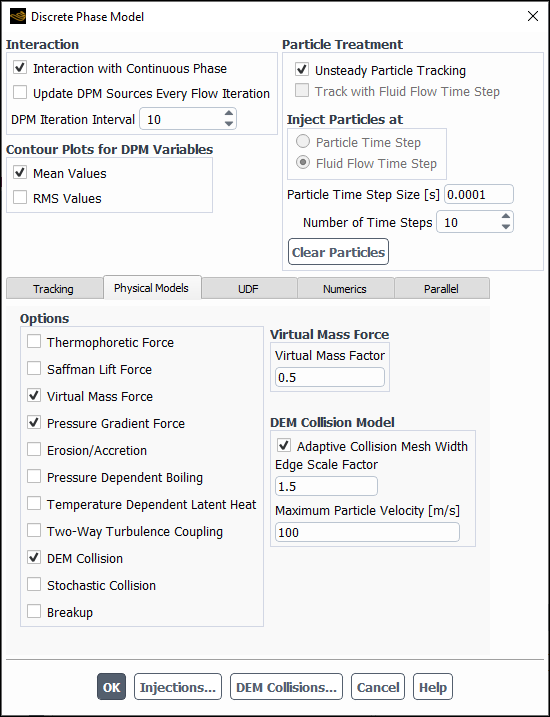
To enable the DEM collision model, select DEM Collision under Options. A detailed description of this model can be found in Discrete Element Method Collision Model in the Theory Guide.
In the Physical Models tab of the Discrete Phase Model dialog box
Specify the settings your model requires under DEM Collision Model.
(Optional) By default, Adaptive Collision Mesh Width is enabled. This adjusts the width of the collision mesh to the largest parcel diameter multiplied by the Edge Scale Factor. If Adaptive Collision Mesh Width is disabled, a fixed Static Collision Mesh Width has to be given in the chosen units of length.
The Maximum Particle Velocity limits the maximum particle velocity to a physically plausible range.
Set up the injection.
 Setup → Models → Discrete Phase → Injections
 New...
In the Set Injection Properties dialog box, select a name from the DEM Collision Partner drop-down list that will serve as the collision partner. A default name using the particle material will be suggested.
Note: Selecting none from the drop-down list indicates that the particles released from this injection do not participate in the DEM collision computation.
If you want to use the rolling friction collision law (see step 4), under the Physical Models tab, enable Particle Rotation for those injections whose particles take part in collisions with rolling friction.
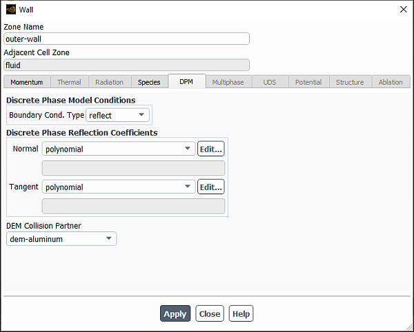
Set the boundary conditions for the discrete phase as you normally would. If the Boundary Cond. Type is reflect, select a name from the DEM Collision Partner drop-down list to designate the collision partner For example, in Figure 24.8: Wall Boundary Condition for the DEM Model, a wall boundary condition will suggest a wall material name, which will designate the collision partner. The name will have a dem- prefix However, if the DEM Collision Partner is none, the wall will reflect particles like any other DPM particles using the settings for the Discrete Phase Reflection Coefficients in the Normal and Tangent directions. These settings generally apply for particles that are not colliding according to DEM, such as massless particles.
Define the particle interaction between the pairs of the collision partners.
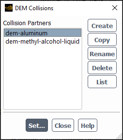
Click the button at the bottom of the Discrete Phase Model dialog box. The DEM Collisions dialog box (Figure 24.9: Collision Dialog Box) will appear where you can manage the collision partners. You can , , , , and collision partners. To define collision laws for a collision partner, select a collision partner from the Collision Partners list and click the button, or simply double-click the collision partner in the list.
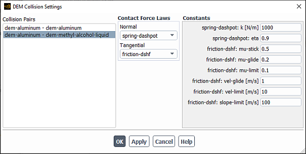
In the DEM Collision Settings dialog box (Figure 24.10: DEM Collision Settings Dialog Box), a list of all the possible Collision Pairs will exist.
Select a pair of collision partners from the Collision Pairs list.
For this pair, select the Contact Force Laws that best describe the collision between these two partners.
The Normal contact force laws that exist are:
spring
spring-dashpot
hertzian
hertzian-dashpot
You can also choose to exclude the contact force law by selecting none.
For the Tangential contact force law (if considered), you can select form the following friction collision laws:
friction-dshf
friction-dshf-rolling (an extension of the friction-dshf friction collision law including rolling friction)
Each of the laws is described in the following sections:
Enter the Constants for the chosen Contact Force Laws. Refer to Theory in the Theory Guide for guidance on how to find reasonable values of the force-law constants.
Repeat for all other collision pairs.
Click or to apply these settings.
Note:
The choice of collision laws does not depend on the order in the pair of collision partners.
Failing to specify a force law for a collision pair implies that respective particles will not collide.
Rolling friction will only be factored in for a particular DEM particle injection if the Particle Rotation option is selected in the Set Injection Properties dialog box (Physical Properties tab).
For parallel calculations, the DEM collision model can be optimized by enabling the hybrid optimization method for DPM. This method balances the load across machines, and, within each machine, the hybrid parallel DPM method is used to make sure the load is balanced by multi-threading. For more information, see the description of the Hybrid Optimization option in the Weighting tab discussion in Partitioning.
The following limitations currently apply when using the DEM collision model:
Axisymmetric geometry cannot be used.
Dynamic mesh motion cannot be used.
The Eulerian wall film model cannot be used.
Shear stress boundary conditions cannot be used at walls.
Marangoni stress boundary condition cannot be used at walls.
DEM particles do not transfer heat from particle to particle during contact.
To better preserve energy during particle collision, the following settings in the Numerics tab are recommended and will be automatically set when DEM Collisions are enabled.
Disable Accuracy Control to ensure that DEM time stepping remains small.
Disable Automated under Tracking Scheme Selection.
Select implicit from the Tracking Scheme drop-down list.
Refer to Numerics for Tracking of the Particles for more information about the settings in the Numerics tab.
In many Lagrangian-Eulerian simulations, the volume fraction of the local particle phase may not be small, and the blocking effect of the particulate phase on the carrier phase may need to be taken into account. See Blockage Effect in the Fluent Theory Guide for more information about the volume displacement effect of particles.
To enable the volume displacement effect of particles, select Volume Displacement (Options group box) in the Physical Models tab of the Discrete Phase Model dialog box.
Once the blocking effect is enabled, you can set the maximum particle volume fraction used to compute the carrier phase volume fraction in Equation 12–522 in the Fluent Theory Guide by issuing the following text command:
define/models/dpm/interaction> max-vf-allowed-for-blockingMaximum DPM volume fraction used in continuous flow (0 1.) [0.95]
For high accuracy solution, using the default value of 0.95 is recommended.
The availability of the DPM volume fraction is automatically triggered by the Ansys Fluent solver.
Note that the blocking effect model has the following limitations:
It is limited to single-phase and homogeneous multiphase (one carrier phase) flows.
The density-based solver is not supported.
The impact of the blocking effect will be strongest in simulations where large particle volume fractions are present in the computational domain, or where the blockage due to the particulate phase may significantly alter the flow structure of the carrier phase. Typical examples are simulations of a particle spray, where the mesh close to the injection nozzle is refined in such a way that the injection nozzle cross-section is discretized by multiple cells, or jet in cross-flow applications, where the blockage effect of the compact liquid jet may enhance the vortex structure in the wake of the jet.
User-defined functions can be used to customize the discrete phase model to include additional body forces, modify interphase exchange terms (sources), calculate or integrate scalar values along the particle trajectory, and incorporate nonstandard erosion rate definitions. More information about user-defined functions can be found in the Fluent Customization Manual.
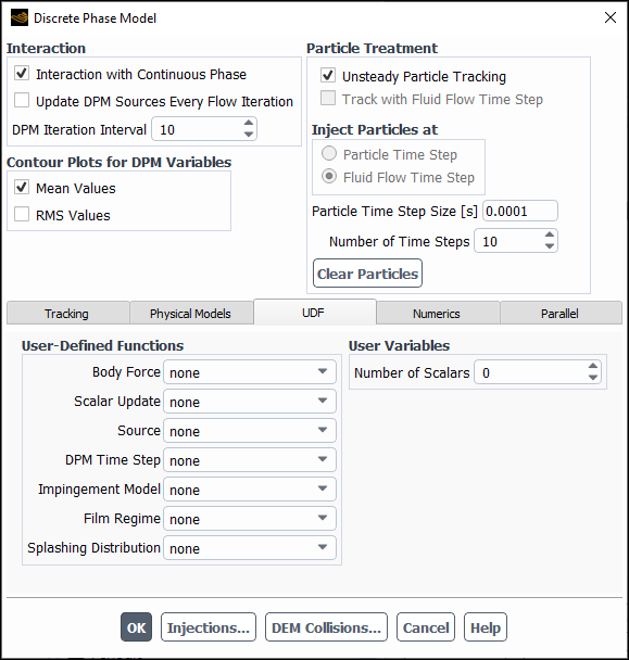
In the Discrete Phase Model Dialog Box, under User-Defined Functions in the UDF tab, there are drop-down lists labeled (see Figure 24.11: The Discrete Phase Model Dialog Box - UDF Tab):
Body Force
Scalar Update
Source
Spray Collide Function
DPM Time Step
Erosion/Accretion (if Erosion/Accretion is enabled under the Physical Models tab)
Impingement Model, Film Regime and Splashing Distribution (if either wall-film is selected for Discrete Phase BC Type in the DPM tab of the Wall dialog box or the Eulerian Wall Film model is enabled).
Note that user-defined Impingement Model and Splashing Distribution will overwrite the impingement/splashing model selected for the Lagrangian or Eulerian wall film boundary condition.
These lists will show available user-defined functions that can be selected to customize the discrete phase model (see Fluent Customization Manual for more information).
In addition, you can specify a Number of Scalars which are allocated to each particle and can be used to store information when implementing your own particle models.
The underlying physics of the Discrete Phase Model is described by ordinary differential equations (ODE) as opposed to the continuous flow which is expressed in the form of partial differential equations (PDE). Therefore, the Discrete Phase Model uses its own numerical mechanisms and discretization schemes, which are completely different from other numerics used in Ansys Fluent.
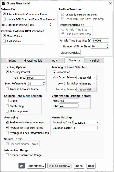
The Numerics tab gives you control over the numerical schemes for particle tracking as well as solutions of heat and mass equations (Figure 24.12: The Discrete Phase Model Dialog Box - Numerics Tab).
Further details are provided in the following sections:
- 24.2.7.1. Numerics for Tracking of the Particles
- 24.2.7.2. Including Coupled Heat-Mass Solution Effects on the Particles
- 24.2.7.3. Tracking in a Reference Frame
- 24.2.7.4. Node Based Averaging of Particle Data
- 24.2.7.5. Linearized Source Terms
- 24.2.7.6. Using the Dynamic Interaction Range
- 24.2.7.7. Staggering of Particles in Space and Time
- 24.2.7.8. Packing Limit
- 24.2.7.9. Under-Relaxing Lagrangian Wall Film Height
To solve equations of motion for the particles, the following tracking numerical schemes are available:
- implicit
uses an implicit Euler integration of Equation 12–1 in the Theory Guide which is unconditionally stable for all particle relaxation times.
- trapezoidal
uses a semi-implicit trapezoidal integration.
- analytic
uses an analytical integration of Equation 12–1 of the Theory Guide where the forces are held constant during the integration.
- runge-kutta
facilitates a 5th order Runge Kutta scheme derived by Cash and Karp [30].
For additional details, see Solution Strategies for the Discrete Phase.
To specify a tracking numerical scheme for your simulation, you can either:
use a single tracking scheme by selecting any of the above numerical schemes from the Tracking Scheme drop-down list (Tracking Scheme Selection group box), or
switch between higher order and lower order tracking schemes using an automated selection based on the accuracy to be achieved and the stability range of each scheme. To use this option, you need to perform the following steps:
Enable Automated (Tracking Scheme Selection group box).
When this option is enabled, the Tracking Scheme drop-down becomes inaccessible, while the High Order Scheme and Low Order Scheme group boxes become available.
Important: The Automated option is available only when Accuracy Control is enabled (Tracking Options group box).
Select trapezoidal or runge-kutta as the High Order Scheme.
Select implicit or analytic as the Low Order Scheme.
During runtime, the solver automatically switches between numerically stable lower order and higher order schemes, which are stable only in a limited range. In situations where the particle is far from hydrodynamic equilibrium, an accurate solution can be achieved very quickly with a higher order scheme, since these schemes need less step refinements for a certain tolerance. When the particle reaches hydrodynamic equilibrium, the higher order schemes become inefficient since their step length is limited to a stable range. In this case, the mechanism switches to a stable lower order scheme and facilitates larger integration steps.
Note:
When DEM Collisions are enabled, Ansys Fluent automatically sets Tracking Scheme to implicit and disables Accuracy Control.
The equation for rotating particle motion (Equation 12–195 in the Fluent Theory Guide) is solved using the Euler implicit discretization scheme.
You can control how accurately the equations need to be solved by using the following settings in the Tracking Options group box:
- Accuracy Control
enables the solution of equations of motion within a specified tolerance. This is done by computing the error of the integration step and reducing the integration step if the error is too large. If the error is within the given tolerance, the integration step will also be increased in the next steps.
- Tolerance
is the maximum relative error that has to be achieved by the tracking procedure. Based on the numerical scheme, different methods are used to estimate the relative error. The implemented Runge-Kutta scheme uses an embedded error control mechanism. The error of the other schemes is computed by comparing the result of the integration step with the outcome of a two step procedure with half the step size.
- Max. Refinements
is the maximum number of step size refinements in one single integration step. If this number is exceeded the integration will be conducted with the last refined integration step size.
By default, the particle heat and mass equations are solved in a segregated manner using an implicit Euler integration over the time step used for the trajectory calculation If you enable the Droplet, Combusting, or Multicomponent particles in the Coupled Heat-Mass Solution group box, Ansys Fluent will solve the corresponding equations using a coupled ODE solver with error tolerance control. The increased accuracy, however, comes at the expense of increased computational time.
To ensure solution accuracy for the Droplet and Multicomponent particles, Ansys Fluent will
automatically switch to the coupled algorithm during the integration
time step when the evaporated mass is greater than the limiting mass
change  (defined in Equation 24–4), or when the particle temperature
change is greater than the limiting temperature change
(defined in Equation 24–4), or when the particle temperature
change is greater than the limiting temperature change  (defined in Equation 24–5).
 | (24–4) |
where  is the particle mass (kg) and
  is the vaporization limiting factor for the mass.
 | (24–5) |
where  is the particle temperature (K),
  is the bulk temperature (K), and
  is the vaporization limiting factor for
the temperature.
is the vaporization limiting factor for
the temperature.
You will enter the Vaporization Limiting Factors for Mass
 and Heat
 . The default values of 0.3 and 0.1 have been determined by systematic testing and are recommended for computations.
Particle tracking is related to a coordinate system. With Track in Absolute Frame enabled in the Tracking Options group box, you can choose to track the particles in the absolute reference frame. All particle coordinates and velocities are then computed in this frame. The forces due to friction with the continuous phase are transformed to this frame automatically.
In rotating flows, it might be appropriate for numerical reasons to track the particles in the relative reference frame. If several reference frames exist in one simulation, then the particle velocities are transformed to each reference frame when they enter the fluid zone associated with this reference frame.
When the impact of particles with walls in multiple rotating reference frames is important, as it is the case with a rotating impeller in a stationary baffled tank, it is necessary to model the flow as a sliding mesh simulation.
In general, the presence of DPM parcels may affect the continuous phase fluid flow meaning that discrete phase source terms and particle data such as fluid drag, temperature, volume fraction, and velocity can be integrated into the flow solver. By default in Ansys Fluent, the effects of a particular DPM parcel are applied only to the cells that intersect with the trajectory of that parcel. As an alternative, Enable Node Based Averaging is offered which distributes the effects of a DPM parcel even into neighboring cells that share at least a mesh node with the cells intersected by the trajectory. This allows a reduction of grid dependency of DPM simulations, since each parcel’s effects on the flow solver are distributed more smoothly across neighboring cells.
You can select Enable Node Based Averaging in the Numerics tab of the Discrete Phase Model dialog box, as shown in Figure 24.12: The Discrete Phase Model Dialog Box - Numerics Tab. For non-DDPM cases, the Enable Node Based Averaging option is not available when the Linearize Source Terms is selected.
When enabled, the node based averaging is applied to particle velocity, particle temperature, particle volume fraction, and DPM concentration. By default, Average DPM Source Terms is also enabled, which applies node averaging to the source terms as well.
When the Dense Discrete Phase Model is being used, the Average DDPM Variables option appears to provide node based averaging for the discrete phase specific variables, such as DDPM particle drag. When Contour Plots for DPM Variables is enabled (Reporting of Discrete Phase Variables), these quantities will also be node averaged.
Average in Each Integration Step should be enabled if you find that the flux report is showing discrepancies for mass flow rates of particles injected into and leaving the domain. This option increases computation time so it is not enabled by default.
Once you have selected Enable Node Based Averaging, you must also select the Averaging Kernel to accumulate the particle related data on the mesh nodes and to redistribute them back to the finite volume cells. The kernel and related settings are specified in the Kernel Settings section of the Discrete Phase Model dialog box. The following kernels are available:
nodes-per-cell
shortest-distance
inverse-distance
gaussian
If you use the gaussian kernel, you must also specify the Gaussian Factor, which determines the width of the Gaussian distribution. The default value is
1.
For details about the averaging and kernel equations, refer to Node Based Averaging in the Theory Guide.
Source terms for discrete phase momentum, energy, and species can be linearized with respect
to the cell variable,  :
:
 | (24–6) |
You can enable source term linearization with the Linearize Source Terms option in the Numerics tab of the Discrete Phase Model dialog box. For non-DDPM cases, the Linearize Source Terms option is not available when the Enable Node Based Averaging is selected.
This linearization strongly increases numerical stability for steady flows. For transient flows, it typically allows the use of a larger time step size and larger under-relaxation factors for the DPM model.
If your simulation involves the species transport model, you can disable the linearization of the species source terms for the discrete phase using the following text command:
define/models/dpm/interaction/linearized-dpm-species-source-terms?
Linearize the species DPM source terms? [yes] no
For non- or partially-premixed combustion cases, the DPM source terms for mixture fractions and inert species (if enabled) can be linearized with respect to the cell variable by enabling the Linearize Source Terms option and issuing the following text command:
define/models/dpm/interaction/linearized-dpm-mixture-fraction-source-terms?yes
Note: As a prerequisite for this linearization, the DPM sources in the mixture fraction equations are cast as a function of the mixture fractions rather than DPM mass. This can be reverted by the following text commands:
define/models/dpm/interaction/replace-dpm-mass-source-by-mixture-fraction?no
Note that entering no will automatically disable the linearization
of the DPM mixture fraction source terms.
The source term linearization can be combined with the Update DPM Sources Every Flow Iteration option (Options for Interaction with the Continuous Phase).
Note the following limitation:
The linearized DPM source terms for mixture fractions and inert species (if enabled) are not compatible with the following UDF macros:
DEFINE_DPM_HEAT_MASS
DEFINE_DPM_LAW
DEFINE_DPM_SOURCE
The linearization will be automatically disabled if any of the above UDFs is used in your case.
DPM cases where the particle diameter may be too large compared to the local mesh cell size can produce an inaccurate solution. To get around this problem, you can enable the Dynamic Interaction Range option in the Interaction Range group box.
When the Dynamic Interaction Range option is enabled, physical models and phase interaction laws (such as drag, fluid temperature, and others) for such large particles are formulated based on freestream conditions of a coarser (or agglomerated) mesh elements. The DPM source terms are distributed over these coarser mesh elements, thus providing more realistic fluid conditions.
This coarser mesh interaction is applied dynamically, that is, the method is only applied if the particle is too large compared to the local cell size at the particle location.
Note the following limitation with the dynamic interaction range model:
The dense discrete phase model (DDPM) is not supported.
Two-sided walls (that is, wall / wall-shadow pairs) with fluid zones on both sides are ignored, that is, the coarser mesh elements stretch out over both sides of the two-sided wall, ignoring its presence.
In order to obtain a better representation of an injector, the particles can be staggered spatially and/or temporally. When particles are staggered spatially, Ansys Fluent randomly samples from the region in which the spray is specified (for example, the sheet thickness in the pressure-swirl atomizer) so that as the calculation progresses, trajectories will originate from the entire region. This allows the entire geometry specified in the atomizer to be sampled while specifying fewer streams in the input dialog box, thus decreasing computational expense.
You can enable injection-specific spatial staggering of the particles by selecting the Stagger Positions option in the Stagger Options group box in the Point Properties tab of the Set Injection Properties dialog box and then, if applicable, specifying Stagger Radius to define the region from which particles are released. For more information, see the appropriate sections for injection-specific point properties.
You can also enable injection-specific spatial staggering of the particles by issuing the following text commands:
define/models/dpm/options/stagger-spatially-atomizer-injections?define/models/dpm/options/stagger-spatially-standard-injections?
When spatial staggering is enabled for non-atomizer injections, a stagger radius must be specified by using the text command:
define/models/dpm/options/stagger-radius
When injecting particles in a transient calculation using a relatively large time step size in relation to the spray event, the particles can clump together in discrete bunches. The clumps do not look physically realistic, though Ansys Fluent calculates the trajectory for each particle as it passes through a cell and the coupling to the gas phase is properly accounted for. To obtain a statistically smoother representation of the spray, the particles can be staggered in time. During the first time step, the particle is tracked for a random percentage of its initial step. This results in a sample of the initial volume swept out by the particle during the first time step and a smoother, more uniform spatial distribution at longer time intervals.
The following setup commands for staggering in time are available in the text user interface (TUI):
stagger-temporally?staggering-factor
The “staggering factor” is applied to temporal staggering only. It is a constant that multiplies the time step size to give the random sampling interval. The staggering factor controls the percentage of every particle’s initial time step that will be sampled. For example, if the staggering factor is 0.5, then the parcels in the injection will be tracked between half and all of their full initial time step. If the staggering factor is 0.1, then the parcels will be tracked between ninety percent and all of their initial time step. If the staggering factor is set to 0.9, the parcels will be tracked between ten percent and all of their initial time step. This allows you to control the amount of smoothing between injections.
The default values for the options in the TUI are spatial staggering for atomizers (including the solid-cone), no temporal staggering and a temporal staggering factor of 1.0. The temporal staggering factor is inactive until the flag for temporal staggering is enabled.
Staggering uses pseudo-random numbers to compute initial particle positions. By default, the initialisation of the random number generator depends on the current iteration and time step numbers, so that the staggered positions of the particles vary between iterations. This helps to distribute DPM source terms more smoothly in the domain if only a limited number of injection streams is used.
In certain situations, the dependence of the initial particle position on the iteration and time step number may cause the overall convergence of the simulation to be slower than when the particle injection positions do not vary between iterations. In such cases, you can use the following text commands to make the random numbers independent of the current time step and iteration numbers:
define/models/dpm/numerics/re-randomize-every-iteration?Update randomness every iteration? [yes]ndefine/models/dpm/numerics/re-randomize-every-timestep?Update randomness every timestep? [yes]no
When using these text commands, make sure that the number of streams used in every injection is sufficiently large.
In transient simulations of granular phases using the DDPM model, DPM parcels may accumulate to unphysically large values, exceeding the packing limit of granular phases. To avoid such behavior, you can enable Enhanced Numerics. This option can be used in combination with the phase-specific option Volume Fraction Approaching Packing Limit (see Defining a Granular Discrete Phase for more information).
As the wall film moves and spreads on the wall faces, under-relaxation is applied to the film height computation. The under-relaxation factor can be specified using the following text command:
define/models/dpm/numerics/underrelax-film-height
A lower under-relaxation factor results in a smoother film appearance, especially closer to the film edge. However, it may distort the film shape, especially for cases where high velocity droplets are impinging on the film. The recommended values range between 0.5 (default) and 0.9.