


While the algebraic slip model supports only small-scale interfaces in the low Stokes number regime, the generalized flow regime framework effectively handles both the small and large-scale interfaces along with the regime transition using special numerical methods. This is important for accurate simulations of multiphase applications that involve various flow regimes, such as free surface flow, bubbly flow, and droplet flow. For more information on how to use the flow regime modeling, refer to Using the Flow Regime Modeling in the Fluent User's Guide.
The generalized flow regime framework distinguishes three different flow regimes (that is, bubbly flow, droplet flow, and free surface flow) and has the following salient features:
Definition of the flow regime by the phase morphology and phase state.
Hybrid morphology specification based on the flow regime detection criterion.
Support of multiple continuous and dispersed phases.
Different sets of methods and defaults for different phase-pair morphologies.
Regime detection via the Algebraic Interfacial Area Density (AIAD) method along with smoothing and filtering techniques.
Ability to use user-defined functions for flow regime modeling.
Regime-based volume fraction discretization.
In the flow regime modeling, phase morphology, which represents the connectivity of the fluid, is classified in the following categories:
Continuous
A phase morphology is classified as continuous if the phase occupies a connected region in the flow domain.
Dispersed
A phase morphology is classified as disperse if the phase occupies disconnected regions in the flow domain.
Hybrid
Hybrid morphology is a dynamic morphology that can behave either as continuous or dispersed depending on the flow regime detection criterion.
Hybrid phase morphology can be observed when:
Phase morphology varies in space and/or time, but there is no real flow regime transition.
There is a regime transition between bubbly flow, droplet flow, and free surface flow.
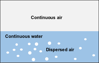
Figure 14.7: Hybrid Phase Morphology with no Regime Transition shows an example of a two-phase flow where air has a hybrid morphology, and water has a continuous morphology. No regime transition occurs in the fluid domain.
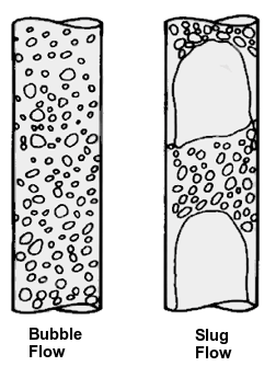
Figure 14.8: Hybrid Phase Morphology with Regime Transition shows an example of a regime transition in a two-phase flow where air behaves as a hybrid phase, while water can behave as a continuous or hybrid phase. The flow regime may transition between bubbly and slug flows.
Both the phase state (liquid or gas) and phase morphology (continuous or dispersed) are critical for the complete definition of the flow regime, such as free surface flow, bubbly, and droplet flow.
Table 14.2: Flow Regime Definitions shows possible regime definitions based on phase morphology and phase states for different flows.
Table 14.2: Flow Regime Definitions
| Flow Regime Classification | Phase Morphology + Phase State |
|---|---|
| Free Surface Flow |
Continuous Liquid/Continuous Liquid Continuous Liquid/Continuous Gas |
| Bubbly Flow |
Continuous Liquid/Dispersed Gas |
| Droplet Flow |
Continuous Gas/Dispersed Liquid Continuous Liquid/Dispersed Liquid |
For a pair of phases with phase indices  and
and  , the following phase-pair interactions can exist:
Hybrid-Hybrid
Continuous-Hybrid
Hybrid-Dispersed
Details for each phase pair interaction are presented below.
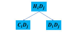
Hybrid-Hybrid Phase Pair Interaction
Interactions possible for the Hybrid-Hybrid phase pair are shown in the diagram below.
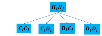
Here,  = continuous regime,
  = dispersed regime,
  = hybrid regime.
In the above diagram,
 is the interaction where both phases behave as continuous (as in the case of
free surface flow). This interaction will be further referred to as is the interaction where both phases behave as continuous (as in the case of
free surface flow). This interaction will be further referred to as  . . |
 is the interaction where phase is the interaction where phase  behaves as continuous, and phase behaves as continuous, and phase  behaves as dispersed (as in the case of bubbly or droplet flow, depending on
the phase states). This interaction will be further referred to as behaves as dispersed (as in the case of bubbly or droplet flow, depending on
the phase states). This interaction will be further referred to as  . . |
 is the interaction where phase behaves as dispersed and phase behaves as continuous (as in the case of droplet or bubbly flow, depending on
the phase states). This interaction will be further referred to as is the interaction where phase behaves as dispersed and phase behaves as continuous (as in the case of droplet or bubbly flow, depending on
the phase states). This interaction will be further referred to as  . . |
 is the interaction where both phases behave as dispersed (as in the case of a
particle-particle interaction, which is only possibly only for flows with more than two
phases). This interaction will be further referred to as is the interaction where both phases behave as dispersed (as in the case of a
particle-particle interaction, which is only possibly only for flows with more than two
phases). This interaction will be further referred to as  . . |
Depending on the flow regime detection criterion, blending factors are calculated to identify various flow regimes that satisfy the following constraint:
 | (14–173) |
where  is the blending factor, and the subscripts represent various flow regimes as
described above.
is the blending factor, and the subscripts represent various flow regimes as
described above.
Area density can be then blended as:
 | (14–174) |
where  is the area density for free surface flow,
  and
and  are the area densities for bubbly flow and droplet flow, respectively, and
 is the area density for particle-particle flow.
For the algebraic slip velocity model with a hybrid-hybrid phase pair, a general form of the slip velocity is given as:
 | (14–175) |
For Continuous-Continuous interaction, velocities of phases and are forced to be equal ( ) by providing zero resistance to the drag, which corresponds to an infinite
drag.
) by providing zero resistance to the drag, which corresponds to an infinite
drag.
For Dispersed-Dispersed interaction,
 | (14–176) |
For Continuous-Dispersed or Dispersed-Continuous interaction, slip velocity is specified by Equation 14–131 and Equation 14–135.
Continuous-Hybrid Phase Pair Interaction
Interactions possible for the Continuous-Hybrid phase pair where phase is continuous, and phase is hybrid are shown in the diagram below.
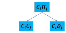
In this case,  , and
, and  .
.
Hybrid-Dispersed Phase Pair Interaction
Interactions possible for the Continuous-Dispersed phase pair where phase is hybrid, and phase is dispersed are shown in the diagram below.
In this case,  and
and  .
.
Ansys Fluent uses the customized variant of the algebraic interfacial area density method proposed by Thomas Höhne et al. [254] for the flow regime detection. In this method, various cosine functions are used to calculate blending factors for flow regime detection.
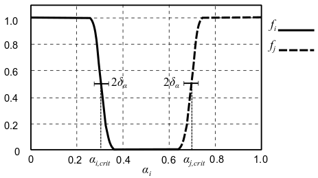
For a pair of phases and , the weighting functions  and
and  are based on the volume fractions and defined as:
 | (14–177) |
where:
 | (14–178) |
In the above equations:
 and and  = volume fractions of phase and phase , respectively = volume fractions of phase and phase , respectively |
 and and  = critical volume fractions of phase and phase , respectively. Default: 0.3 = critical volume fractions of phase and phase , respectively. Default: 0.3 |
 = volume fraction width for the intermediate transition. Default: 0.05. = volume fraction width for the intermediate transition. Default: 0.05.
|
Figure 14.9: Weighting Functions  and
and  (adapted from [254]) shows a plot of the weighting functions
  and
and  against the volume fraction.
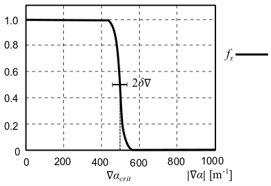
The weighting function of the phase boundary  based on the volume fraction gradient is expressed as:
 | (14–179) |
where:
 | (14–180) |
 | (14–181) |
 | (14–182) |
 | (14–183) |
In Equation 14–183,  is the fraction of the critical gradient for defining the intermediate
transition width (default: 0.1).
is the fraction of the critical gradient for defining the intermediate
transition width (default: 0.1).
In Equation 14–182,  is the cell number for determining the interfacial width for free surface
flow, and
is the cell number for determining the interfacial width for free surface
flow, and  is the cell size expressed as:
 | (14–184) |
Figure 14.10: Weighting Function  (adapted from [254]) shows the weighting function over the critical gradient of the phase fraction
  .
.
For the detection of a phase boundary by the criteria of the volume fraction and its
gradient, the weighting function of the phase boundary  is used:
 | (14–185) |
The flow regime blending factors are then calculated as:
 | (14–186) |
 | (14–187) |
 | (14–188) |
where
 | (14–189) |