


The dialog boxes described in this section can be accessed through the ribbon, from the tabs other than the File ribbon tab.
- 52.2.1. 1D Simulation Library Dialog Box
- 52.2.2. Activate Cell Zones Dialog Box
- 52.2.3. Adaption Criteria Settings Dialog Box
- 52.2.4. Adjacency Dialog Box
- 52.2.5. Advanced Options Dialog Box
- 52.2.6. Aerodamping (Influence Coefficient Method) Report Definition Dialog Box
- 52.2.7. Aerodamping (Travelling Wave Method) Report Definition Dialog Box
- 52.2.8. Animation Definition Dialog Box
- 52.2.9. Application About to Exit Dialog Box
- 52.2.10. Auto Partition Mesh Dialog Box
- 52.2.11. Automatic Mesh Adaption Dialog Box
- 52.2.12. Cell Count Report Definition Dialog Box
- 52.2.13. Cell Register Display Options Dialog Box
- 52.2.14. Compiled UDFs Dialog Box
- 52.2.15. Conduction Layers Dialog Box
- 52.2.16. Conduction Manager Dialog Box
- 52.2.17. Contours Dialog Box
- 52.2.18. Convergence Conditions Dialog Box
- 52.2.19. Create Mesh Interfaces
- 52.2.20. Create/Edit Mesh Interfaces Dialog Box
- 52.2.21. Create/Edit Turbo Interfaces Dialog Box
- 52.2.22. Curvilinear Coordinate System Dialog Box
- 52.2.23. Custom Field Function Calculator Dialog Box
- 52.2.24. Custom Laws Dialog Box
- 52.2.25. Dashboard Definition Dialog Box
- 52.2.26. Deactivate Cell Zones Dialog Box
- 52.2.27. Define Control Points Dialog Box
- 52.2.28. Delete Cell Zones Dialog Box
- 52.2.29. Display Options - Adaption Dialog Box
- 52.2.30. Display States Dialog Box
- 52.2.31. DPM Report Definition Dialog Box
- 52.2.32. DPM Source Report Definition Dialog Box
- 52.2.33. Drag Report Definition Dialog Box
- 52.2.34. DTRM Graphics Dialog Box
- 52.2.35. DTRM Rays Dialog Box
- 52.2.36. Edit Gap Region Dialog Box
- 52.2.37. Edit Mesh Interfaces Dialog Box
- 52.2.38. Edit Report File Dialog Box
- 52.2.39. Edit Report Plot Dialog Box
- 52.2.40. Execute on Demand Dialog Box
- 52.2.41. Expression Dialog Box
- 52.2.42. Expression Editor Dialog Box
- 52.2.43. Expression Manager Dialog Box
- 52.2.44. Expression Report Definition Dialog Box
- 52.2.45. Expression Volume Dialog Box
- 52.2.46. Face Count Report Definition Dialog Box
- 52.2.47. Field Function Definitions Dialog Box
- 52.2.48. Flux Report Definition Dialog Box
- 52.2.49. Force Report Definition Dialog Box
- 52.2.50. Fuse Face Zones Dialog Box
- 52.2.51. Gap Model Dialog Box
- 52.2.52. General Adaption Controls Dialog Box
- 52.2.53. Generalized/Modal Force Report Definition Dialog Box
- 52.2.54. Geometry Based Adaption Controls Dialog Box
- 52.2.55. Geometry Based Adaption Dialog Box
- 52.2.56. Import Particle Data Dialog Box
- 52.2.57. Imprint Surface Dialog Box
- 52.2.58. Improve Mesh Dialog Box
- 52.2.59. Injections Dialog Box
- 52.2.60. Input Summary Dialog Box
- 52.2.61. Interface Creation Options Dialog Box
- 52.2.62. Interpreted UDFs Dialog Box
- 52.2.63. Iso-Clip Dialog Box
- 52.2.64. Iso-Surface Dialog Box
- 52.2.65. Lift Report Definition Dialog Box
- 52.2.66. Line Integral Convolutions Dialog Box
- 52.2.67. Line/Rake Surface Dialog Box
- 52.2.68. Manual Mesh Adaption Dialog Box
- 52.2.69. Manage Adaption Criteria Dialog Box
- 52.2.70. Manage Geometry-Based Adaption Dialog Box
- 52.2.71. Manage Sponge Layers Dialog Box
- 52.2.72. Mapped Interface Options Dialog Box
- 52.2.73. Material Editor Dialog Box
- 52.2.74. Measure Dialog Box
- 52.2.75. Merge Zones Dialog Box
- 52.2.76. Mesh Interfaces Dialog Box
- 52.2.77. Mesh Morpher/Optimizer Dialog Box
- 52.2.78. Mixing Planes Dialog Box
- 52.2.79. Moment Report Definition Dialog Box
- 52.2.80. Motion Settings Dialog Box
- 52.2.81. Multi Edit Dialog Box
- 52.2.82. New Report File Dialog Box
- 52.2.83. New Report Plot Dialog Box
- 52.2.84. Objective Function Definition Dialog Box
- 52.2.85. Optimization History Monitor Dialog Box
- 52.2.86. Parallel Connectivity Dialog Box
- 52.2.87. Parameter Bounds Dialog Box
- 52.2.88. Particle Tracks Dialog Box
- 52.2.89. Partition Surface Dialog Box
- 52.2.90. Partitioning and Load Balancing Dialog Box
- 52.2.91. Pathlines Dialog Box
- 52.2.92. PCB Model Dialog Box
- 52.2.93. Plane Surface Dialog Box
- 52.2.94. Point Surface Dialog Box
- 52.2.95. Quadric Surface Dialog Box
- 52.2.96. Raytracing Display Dialog Box
- 52.2.97. Reduced Order Model Dialog Box
- 52.2.98. Reference Frame Dialog Box
- 52.2.99. Replace Cell Zone Dialog Box
- 52.2.100. Report Definitions Dialog Box
- 52.2.101. Report File Definitions Dialog Box
- 52.2.102. Report Plot Definitions Dialog Box
- 52.2.103. Residual Monitors Dialog Box
- 52.2.104. Rotate Mesh Dialog Box
- 52.2.105. S2S Information Dialog Box
- 52.2.106. Select UDM Zones Dialog Box
- 52.2.107. Select Window Dialog Box
- 52.2.108. Separate Cell Zones Dialog Box
- 52.2.109. Separate Face Zones Dialog Box
- 52.2.110. Set Injection Properties Dialog Box
- 52.2.111. Set Multiple Injection Properties Dialog Box
- 52.2.112. Sponge Layer Dialog Box
- 52.2.113. Structural Point Surface Dialog Box
- 52.2.114. Surface Meshes Dialog Box
- 52.2.115. Surface Rendering Properties Dialog Box
- 52.2.116. Surface Report Definition Dialog Box
- 52.2.117. Surfaces Dialog Box
- 52.2.118. Thread Control Dialog Box
- 52.2.119. Time Averaged Explicit Thermal Coupling Dialog Box
- 52.2.120. Transform Surface Dialog Box
- 52.2.121. Translate Mesh Dialog Box
- 52.2.122. Turbo 2D Contours Dialog Box
- 52.2.123. Turbo Averaged Contours Dialog Box
- 52.2.124. Turbo Averaged XY Plot Dialog Box
- 52.2.125. Turbo Options Dialog Box
- 52.2.126. Turbo Report Dialog Box
- 52.2.127. Turbo Topology Dialog Box
- 52.2.128. UDF Library Manager Dialog Box
- 52.2.129. User-Defined Fan Model Dialog Box
- 52.2.130. User-Defined Function Hooks Dialog Box
- 52.2.131. User-Defined Memory Dialog Box
- 52.2.132. User Defined Report Definition Dialog Box
- 52.2.133. User-Defined Scalars Dialog Box
- 52.2.134. Vectors Dialog Box
- 52.2.135. Volume Report Definition Dialog Box
- 52.2.136. Warning Dialog Box
- 52.2.137. Zone Surface Dialog Box
- 52.2.138. Zone Type Color and Material Assignment Dialog Box
The 1D Simulation Library dialog box allows you to set parameters related to coupling between Ansys Fluent and GT-POWER or WAVE. See Coupling Boundary Conditions with GT-POWER or Coupling Boundary Conditions with WAVE for details about the items below.
![]() User Defined → Model Specific
→ 1D Coupling...
User Defined → Model Specific
→ 1D Coupling...
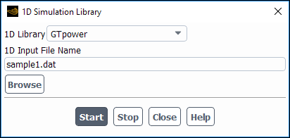
Controls
- 1D Library
specifies the type of library to be used. (Currently only GTpower and WAVE are available.)
- 1D Input File Name
specifies the name of the GT-POWER or WAVE input file.
- Start
starts up GT-POWER or WAVE and generates Ansys Fluent user-defined functions for each boundary in the input file.
- Stop
unlinks the shared library.
The Activate Cell Zones dialog box allows you to activate a single cell zone or multiple zones. See Activating Zones for details.
![]() Domain → Zones
→ Activate...
Domain → Zones
→ Activate...
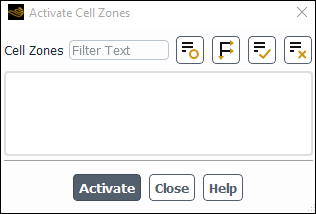
Controls
- Cell Zones
contains a list of cell zones from which you can select the zone to be activated.
- Activate
activates the selected cell zones.
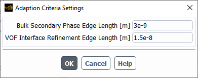
The Adaption Criteria Settings dialog box allows you to complete the setup of an adaption criterion when you have made a selection from the Predefined Criteria drop-down list in the Manual Mesh Adaption Dialog Box or Automatic Mesh Adaption Dialog Box; the Adaption Criteria Settings dialog box opens automatically, and is used to define necessary settings or parameters in the refinement / coarsening criterion expression or overset adaption settings. See Refining and Coarsening and Predefined Criteria for Adaption for details.
Controls
(when setting up the Cell Distance predefined criterion under Boundary Layer...)
- Boundary Zones
specifies the boundary zones where adjacent cell layers will be split for boundary layer adaption. The selections are used in a boundary register named boundary_cell_distance that is selected in the Refinement Criterion field in the Manual Mesh Adaption Dialog Box.
- Cell Layers to Split
specifies the number of cell layers that will be split for boundary layer adaption. The value you enter is used in a boundary register named boundary_cell_distance that is selected in the Refinement Criterion field in the Manual Mesh Adaption Dialog Box.
(when setting up the Flame Indicator predefined criterion under Combustion...)
- Include Vortex Indicator
specifies that the magnitude of vorticity is included as part of the criteria for refinement and coarsening.
- Spark Region Refinement
enables refinement in a temporary spherical spark region at the start of the simulation (which will then later be coarsened back to the original mesh).
- Time
sets the maximum time during which refinement is applied to the spark region, as part of the Spark Region Refinement option. The value you enter will automatically update an expression named spark_<ID>, which is a parameter in the flame_refinement_<ID> expression used in the Refinement Criterion field in the Manual Mesh Adaption Dialog Box or Automatic Mesh Adaption Dialog Box.
- Centroid X
sets the x-coordinate for the center of the spark region as part of the Spark Region Refinement option. The value you enter will automatically update a cell register named spark_region, which is used in an expression named spark_<ID> that is a parameter in the flame_refinement_<ID> expression used in the Refinement Criterion field in the Manual Mesh Adaption Dialog Box or Automatic Mesh Adaption Dialog Box.
- Centroid Y
sets the y-coordinate for the center of the spark region as part of the Spark Region Refinement option. The value you enter will automatically update a cell register named spark_region, which is used in an expression named spark_<ID> that is a parameter in the flame_refinement_<ID> expression used in the Refinement Criterion field in the Manual Mesh Adaption Dialog Box or Automatic Mesh Adaption Dialog Box.
- Centroid Z
sets the z-coordinate for the center of the spark region as part of the Spark Region Refinement option. The value you enter will automatically update a cell register named spark_region, which is used in an expression named spark_<ID> that is a parameter in the flame_refinement_<ID> expression used in the Refinement Criterion field in the Manual Mesh Adaption Dialog Box or Automatic Mesh Adaption Dialog Box.
- Radius
sets the radius of the spherical spark region as part of the Spark Region Refinement option. The value you enter will automatically update a cell register named spark_region, which is used in an expression named spark_<ID> that is a parameter in the flame_refinement_<ID> expression used in the Refinement Criterion field in the Manual Mesh Adaption Dialog Box or Automatic Mesh Adaption Dialog Box.
(when setting up the Volume of Fluid predefined criterion under Multiphase...)
- Minimum Cell Length Scale
sets the minimum cell length scale for refinement. By default this is set to the minimum cell edge length in the initial mesh. It is used to automatically update the cell volume in an expression named vof_refinement_<ID> that is used in the Refinement Criterion field in the Manual Mesh Adaption Dialog Box or Automatic Mesh Adaption Dialog Box.
(when setting up the VOF-to-DPM [Generic] predefined criterion under Multiphase...)
- Number of Cells Across Resolved Droplet
sets the number of cells across the resolved droplet (
 ). It is used to automatically update the cell volume (as
described in the definition that follows) used in the
vof_to_dpm_refinement_<ID>
expression that is used in the Refinement Criterion field
in the Manual Mesh Adaption Dialog Box or Automatic Mesh Adaption Dialog Box.
). It is used to automatically update the cell volume (as
described in the definition that follows) used in the
vof_to_dpm_refinement_<ID>
expression that is used in the Refinement Criterion field
in the Manual Mesh Adaption Dialog Box or Automatic Mesh Adaption Dialog Box.- Minimum Resolved Droplet Diameter
sets the minimum diameter of droplets that are resolved in the simulation (
 ). By default this is set to the minimum cell edge length in
the initial mesh. It is used (with the Number of Cells Across Resolved
Droplet setting) to automatically update the cell volume used in the
vof_to_dpm_refinement_<ID>
expression, by setting it to
). By default this is set to the minimum cell edge length in
the initial mesh. It is used (with the Number of Cells Across Resolved
Droplet setting) to automatically update the cell volume used in the
vof_to_dpm_refinement_<ID>
expression, by setting it to  . This expression is then used in the Refinement
Criterion field in the Manual Mesh Adaption Dialog Box
or Automatic Mesh Adaption Dialog Box.
. This expression is then used in the Refinement
Criterion field in the Manual Mesh Adaption Dialog Box
or Automatic Mesh Adaption Dialog Box.
(when setting up the VOF-to-DPM [Advanced] predefined criterion under Multiphase...)
- Bulk Secondary Phase Edge Length
specifies an edge length that is cubed in order to define the minimum cell volume that initiates refinement in the secondary phase. This volume is used in an expression named vof_to_dpm_refinement_1 that is used in the Refinement Criterion field in the Manual Mesh Adaption Dialog Box or Automatic Mesh Adaption Dialog Box.
- VOF Interface Refinement Edge Length
specifies an edge length that is cubed in order to define minimum / maximum cell volume that initiates refinement / coarsening at the VOF interface. This volume is used in expressions named vof_to_dpm_refinement_1 and vof_to_dpm_coarsening_1, which are then used in the Refinement Criterion and Coarsening Criterion fields, respectively, in the Manual Mesh Adaption Dialog Box or Automatic Mesh Adaption Dialog Box.
(when setting up the Overset predefined criterion)
- Orphan Adaption
enables adaption that attempts to remove orphan cells. For details, see Marking for Orphan Adaption.
- Size Adaption
enables adaption that reduces size mismatches between donor and receptor cells. For details, see Marking for Size Adaption.
- Maximum Length Scale Ratio
sets the threshold (
 ) used as part of the Size Adaption option
to determine which cells are marked for adaption based on donor-receptor cell
size differences. This is set to 3 by default.
) used as part of the Size Adaption option
to determine which cells are marked for adaption based on donor-receptor cell
size differences. This is set to 3 by default.- Gap Adaption
enables adaption that increases the mesh resolution in gaps as needed (in order to prevent the creation of orphan cells). For details, see Marking for Gap Adaption.
- Gap Resolution
specifies the target (minimum) gap resolution used as part of the Gap Adaption option when marking cells for gap adaption. This is set to 4 by default.
- Coarsening
enables the coarsening of the mesh when mesh refinement is no longer needed.
(when setting up the Goal-Based Error Indicator predefined criterion under Aerodynamics...)
- Set Up Goal...
Opens the Adjoint Observables dialog box where you can select, edit, or create the desired observable.
- Skip Initial Adjoint Advancement Before Adaption
When enabled, if the adjoint solution is calculated, the mesh adaption will ignore the computationally expensive initial adjoint iterations which are specified by Initial Adjoint Iterations before Adaption.
- Initial Adjoint Iterations Before Adaption
This specifies the number of adjoint iterations in the initial adjoint calculation before the first mesh adaption.
- Adjoint Iterations Before Adaption
This specifies the number of adjoint iterations during the adjoint calculation before each mesh adaption.
- Number of Modes for Adjoint Advancement
This specifies the number of modes in the Krylov subspace used to approximate the solution. A larger value will help to converge the adjoint solution at the expense of memory cost and potentially more computational time.
- Smoothing Steps Before Adaption
A larger value will lead to smoother adaption.
- Reset Adaption History
Deletes any previous adaption history.
- Print Adaption History
Prints the goal-based adaption history in the console.
The Adjacency dialog box allows you to identify, display, and rename face zones based on their adjacency to a selected cell zone. You can also rename cell zones by zone type and ID, by wildcard, and by adding prefixes/suffixes. See Managing Adjacent Zones for details.
![]() Domain → Zones
→ Adjacency...
Domain → Zones
→ Adjacency...
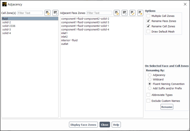
Controls
- Cell Zone(s)
contains a list of the cell zones for which you can find adjacent face zones.
- Adjacent Face Zones
contains a list of the face zones that are adjacent to the selected cell zones.
- Options
contains relevant options for adjacency.
- Multiple Cell Zones
allows you to select multiple cell zones at once. The zones listed in Adjacent Face Zones will be the union of all zones adjacent to the selected cell zones.
- Rename Face Zones
allows you to rename selected face zones based on adjacency, zone type, wild card, or add a prefix/suffix.
- Rename Cell Zones
allows you to rename selected cell zones based zone type and ID, wild card, or by adding a prefix/suffix.
- Draw Default Mesh
brings up the Mesh Display Dialog Box where you can specify zones of the mesh to be permanently displayed as you display or hide face zones from within the Adjacency dialog box. This can be helpful in cases where the mesh is very complex. If this option is not enabled, only the zones selected in Adjacent Face Zones will be displayed when you click Display Face Zones.
- On Selected Face Zones
contains controls for renaming face zones that are selected in Adjacent Face Zones. For details on the renaming methods, refer to Renaming Zones Using the Adjacency Dialog Box.
- Renaming By:
contains options for how you can rename surfaces.
- Adjacency
renames the selected face zones incorporating the name of the adjacent cell zone and the face zone type when you click .
- Fluent Naming Convention
renames the selected surface to be a combination of the surface type and the surface ID when you click . Cell zones are renamed to be a combination of the zone type and the zone ID.
- Wildcard
renames the selected face zones or cell zones based on a pattern match string in the From field and a replacement string in the To field.
- Add Suffix and/or Prefix
adds the provided text in the Suffix or Prefix field to either the beginning or end of the selected zone name(s). Click to add the provided text at the end of the name and click to add the provided text at the beginning of the name.
- Abbreviate Types
uses abbreviations for the zone types when renaming rather than the full zone type text.
- Exclude Custom Names
excludes from renaming any zones that do not match a recognized naming pattern. This can be useful to prevent inadvertently replacing a meaningful name.
- Displace Face Zones
displays the face zones selected in Adjacent Face Zones.
The Advanced Options dialog box provides advanced options for a simulation that uses the gap model to simulate flow through narrow gaps that open or close over time (such as in a valve). It is opened by clicking in the Gap Model Dialog Box. See also Controlling Flow in Narrow Gaps for Valves and Pumps.
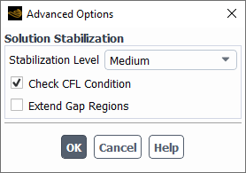
Controls
- Solution Stabilization
allows you to define solution stabilization settings for the gap model.
- Stabilization Level
allows you to define the level of solution stabilization for the gap model simulation. For each level, the solver adjusts the numerical settings, discretization schemes, under-relaxations, AMG settings, and so on, and controls the flow behavior in vicinity of the gap regions. The cost of computation increases with higher levels. Note that these changes are applied globally to all gap regions, and a level other than None will override the local stabilization applied by default to flow-modeling regions that use the Sponge Layer method.
- Check CFL Condition
enables the automatic determination of a desirable acoustic Courant (CFL) number based on the selected Stabilization Level, and then provides a warning message in the console if this CFL number would require you to specify a smaller time step for the calculation in order to improve the solver stability.
- Extend Gap Regions
enables the extending of the gap regions by including additional cells in the vicinity of the gap interfaces during marking. This is useful when the default shape of the marked cells is negatively affecting solution stability or convergence behavior.
For more details, see ICM Method Post-processing.
![]() Solution → Reports
→ Definitions → New
→ Aeromechanics Report → Aerodamping
(Influence Coefficient Method)...
Solution → Reports
→ Definitions → New
→ Aeromechanics Report → Aerodamping
(Influence Coefficient Method)...
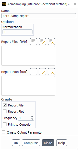
Controls
- Name
specifies the name of the report definition.
- Options
contains options for your aerodamping report definition.
- Normalization
Sets the normalization factor for the damping value.
- Report Files
lists all of the report files where you can write the report definition data.
- Report Plots
lists all of the report plots where you can plot the report definition data (assuming this report has the same units as the other report definitions included in the selected report plot).
- Create
- Report File
creates a new report file that includes this report definition.
- Report Plot
creates a new report plot that includes this report definition.
- Frequency
specifies how frequently the report definition is written, plotted, or printed to the console.
- Print to Console
prints the value of the report definition to the console.
- Create Output Parameter
creates an output parameter for this report definition with the name
<report definition name>-op.- OK
creates the report definition.
- Compute
computes the value of the report definition at the selected zone(s) and prints to the console.
For more details, see TWM Method Post-processing.
![]() Solution → Reports
→ Definitions → New
→ Aeromechanics Report → Aerodamping
(Travelling Wave Method)...
Solution → Reports
→ Definitions → New
→ Aeromechanics Report → Aerodamping
(Travelling Wave Method)...
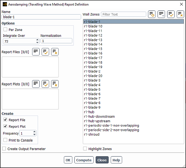
Controls
- Name
specifies the name of the report definition.
- Options
contains options for your aerodamping report definition.
- Per Zone
If you are modeling multiple (main) blades, enables the damping value to be calculated for each dynamic mesh zone (which encompasses one main blade and possibly accompanying splitter blades).
- Integrate Over
sets the number of time steps over which to integrate when calculating the damping value; a suggested value is the number of time steps per period..
- Normalization
Sets the normalization factor for the damping value.
- Report Files
lists all of the report files where you can write the report definition data.
- Report Plots
lists all of the report plots where you can plot the report definition data (assuming this report has the same units as the other report definitions included in the selected report plot).
- Create
- Report File
creates a new report file that includes this report definition.
- Report Plot
creates a new report plot that includes this report definition.
- Frequency
specifies how frequently the report definition is written, plotted, or printed to the console.
- Print to Console
prints the value of the report definition to the console.
- Create Output Parameter
creates an output parameter for this report definition with the name
<report definition name>-op.- Wall Zones
contains a selectable list of valid walls zones for aerodamping report.
- OK
creates the report definition.
- Compute
computes the value of the report definition at the selected zone(s) and prints to the console.
The Animation Definition dialog box allows you to specify a graphics object that will be captured during the solution calculation so that it may be played back as an animation during postprocessing.
![]() Solution → Activities
→ Create → Solution
Animations...
Solution → Activities
→ Create → Solution
Animations...
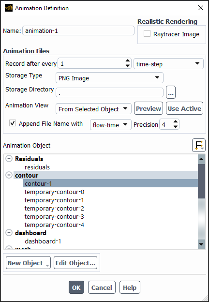
Controls
- Name
name of the animation definition.
- Realistic Rendering
option for enhancing the appearance of the animation object by using a raytracer for realistic lighting effects.
- Raytracer Image
indicates that animation images will use a raytracing renderer for enhanced image quality. Refer to Realistic Rendering Using Raytracing for additional information on raytracing.
- Animation Files
controls for how animation files are stored.
- Record after every
specifies the frequency that images are captured during the calculation. You can select whether the frequency is Iteration, Time Step (transient only) or Flow Time (transient only) from the drop-down.
- Storage Type
drop-down list with the available formats for storing the animation images.
- None
no images are saved. This option is intended for use with embedded window dashboards (Embedded Graphics Window Dashboards).
- In Memory
the image files associated with the animation will lost when you exit Fluent.
- PPM Image
Fluent will save the animation images in PPM Image format (
.ppm), which is 2D.- HSF File
Fluent will save the animation images in HSF file format (
.hsf), which is 3D.- PNG Image
Fluent will save the animation images in PNG file format (
.png), which is 2D.- JPEG Image
Fluent will save the animation images in JPEG file format (
.jpg), which is 2D.- TIFF Image
Fluent will save the animation images in tagged image file format (TIFF—
.tif), which is 2D.
- Storage Directory
shows the location where the animation images will be stored if the Storage Type is set to any of the types other than In Memory.
Note: Animation files are written to the same directory as the case file, by default. This is stored as a relative path, represented by a dot (.), so that when a case file is shared, animation files are written to an appropriate location.
If you manually specify a path, then what you are specifying is an absolute path that will not automatically be updated if the case file is shared or run from another directory.
- Animation View
specifies the animation object orientation that will be used when the animation images are capture during the calculation.
- views drop-down
list with all of the defined views.
- Preview
displays the selected animation object in a reserved graphics window.
- Use Active
saves the current view in the active graphics window and automatically selects it for use in the animation definition.
- Append File Name with
indicates that the Name of the animation files will have either the time-step, flow-time, or iteration appended. The drop-down menu allows you to specify which one.
- Precision
indicates the number of decimal places included when the flow-time is appended.
- Animation Object
lists the defined graphics objects that may be selected for animation.
- New Object
drop-down list allowing you to create new graphics objects for animating.
Mesh... opens the Mesh Display Dialog Box.
Contours... opens the Contours Dialog Box.
Vectors... opens the Vectors Dialog Box.
Pathlines... opens the Pathlines Dialog Box.
Particle Tracks... opens the Particle Tracks Dialog Box.
Scene... opens Figure 40.50: The Scene Dialog Box.
XY Plot... opens the Solution XY Plot Dialog Box.
Report Plot... opens the New Report Plot Dialog Box.
allows you to edit the selected graphics object.
creates the animation definition and/or saves settings changes and closes the dialog box.
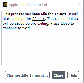
The Application About to Exit dialog box gives you chance to stop the Ansys Fluent session from saving and exiting as the session approaches the idle timeout set in the Set Idle Timeout Dialog Box. Refer to Having the Session Close After Sitting Idle for additional information.
Controls
- Change Idle Timeout...
opens the Set Idle Timeout Dialog Box.
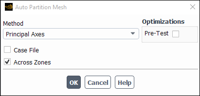
The Auto Partition Mesh dialog box allows you to set the parameters for automatic partitioning when reading an unpartitioned mesh into the parallel solver. See Partitioning the Mesh Automatically for details.
![]() Parallel → General → Auto Partition...
Parallel → General → Auto Partition...
Controls
- Method
contains a drop-down list of the recursive partition methods that can be used to create the mesh partitions. The choices include the Cartesian Axes, Cartesian Strip, Cartesian X-Coordinate, Cartesian Y-Coordinate, Cartesian Z-Coordinate, Cartesian R Axes, Cartesian RX-Coordinate, Cartesian RY-Coordinate, Cartesian RZ-Coordinate, Cylindrical Axes, Cylindrical R-Coordinate, Cylindrical Theta-Coordinate, Cylindrical Z-Coordinate, Metis, Polar Axes, Polar R-Coordinate, Polar Theta-Coordinate, Principal Axes, Principal Strip, Principal X-Coordinate, Principal Y-Coordinate, Principal Z-Coordinate, Spherical Axes, Spherical Rho-Coordinate, Spherical Theta-Coordinate, and Spherical Phi-Coordinate techniques, which are described in Mesh Partitioning Methods.
- Case File
allows you to use a valid existing partition section in a case file (that is, one where the number of partitions in the case file divides evenly into the number of compute nodes). You need to turn off the Case File option only if you want to change other parameters in the Auto Partition Mesh dialog box.
- Across Zones
allows partitions to cross zone boundaries (the default). If turned off, it will restrict partitioning to within each cell zone. This is recommended only when cells in different zones require significantly different amounts of computation during the solution phase, for example if the domain contains both solid and fluid zones.
- Optimizations
contains an option to enable pre-testing.
- Pre-Test
instructs Fluent to test all coordinate directions and choose the one which yields the fewest partition interfaces for the final bisection. Note that this option is available only when you choose Principal Axes or Cartesian Axes as the partitioning method.
The Automatic Mesh Adaption dialog box allows you to create and edit criteria that Fluent will use to adapt your mesh during a calculation. See Refining and Coarsening for details.
![]() Domain → Adapt →
Automatic...
Domain → Adapt →
Automatic...
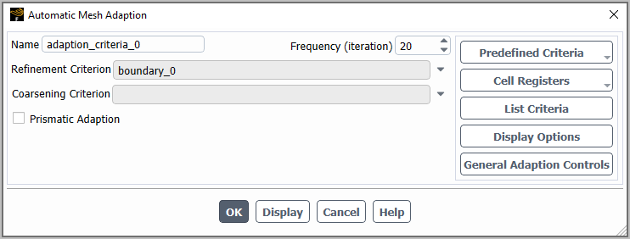
Controls
- Name
specifies the name of the adaption criteria.
- Frequency
defines the frequency of the adaption that will be applied for this criteria during the calculation.
- Refinement Criterion
specifies the cell register or expression that Fluent will use during the calculation to determine which cells to refine.
- Coarsening Criterion
specifies the cell register or expression that Fluent will use during the calculation to determine which cells to coarsen.
- Prismatic Adaption
specifies that prismatic cells are adapted anisotropically. This option is only available with the PUMA adaption method.
allows you to select from a list of commonly used criteria for adapting the mesh (for a description of the list, see Predefined Criteria for Adaption); if one is selected, Fluent will automatically generate cell registers and/or expressions for refinement and coarsening, and define the settings in the Automatic Mesh Adaption dialog box and General Adaption Controls Dialog Box as needed. Depending on your selection, you may be prompted to complete the setup by defining fields in the Adaption Criteria Settings Dialog Box.
allows you to create new cell registers and manage existing ones, which may then be selected from the Refinement Criterion and/or Coarsening Criterion drop-down lists.
prints to the console the number of cells marked for refinement, the number of cells marked for coarsening, and the number marked for both operations.
opens the Display Options - Adaption Dialog Box.
opens the General Adaption Controls Dialog Box, where you can specify the general settings that Fluent uses when adapting the mesh.
The Cell Count Report Definition dialog box allows you to create a report definition for the reporting of a cell count (that is, the number of cells within one or more cell zones), as described in Mesh Report Definitions.
![]() Solution → Reports
→ Definitions → New
→ Mesh Report → Cell Count...
Solution → Reports
→ Definitions → New
→ Mesh Report → Cell Count...
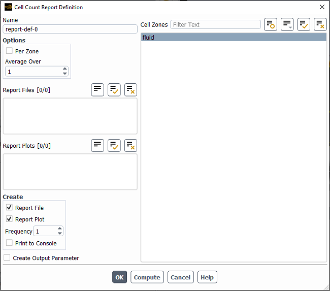
Controls
- Name
specifies the name of the report definition.
- Options
- Per Surface
enables the reporting of the cell count individually for each of the selected zones (rather than reporting the sum from all of the selected zones).
- Average Over
specifies the number of iterations / time steps over which the cell count is averaged when written, plotted, and/or printed. The default value of
1means that no averaging is performed (that is, only the current cell count is reported), and higher values yields a running average. When the iteration / time step number is lower than the specified value, Fluent calculates the average of the available cell count values.- Retain Instantaneous Values
enables the retention of instantaneous values in any report file definition or report plot definition that is associated with this report definition. This option is only available if Average Over is set to a value greater than
1.
- Report Files
allows you to select existing report file definitions to which you want to write cell count data from this report definition.
- Report Plots
allows you to select existing report plot definitions to which you want to include cell count data from this report definition. Note that the units used in these report plots may not be suitable for the cell count data.
- Create
- Report File
creates a new report file definition for the data from this report definition.
- Report Plot
creates a new report plot definition for the data from this report definition.
- Frequency
specifies how frequently the report definition is written, plotted, and/or printed to the console.
- Print to Console
enables the printing of the cell count data from this report definition to the console during the calculation.
- Create Output Parameter
creates an output parameter for this report definition with the name <report_definition_name>
-op.- Cell Zones
allows you to select the cell zones for which you want to report the number of cells.
- OK
creates / saves the report definition.
- Compute
computes the cell count within the selected zone(s) and prints to the console.
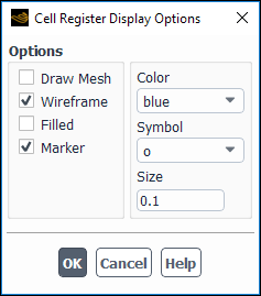
The Cell Register Display Options dialog box allows you to customize the display of cell registers.
You can access this dialog box by clicking in any of the cell register dialog boxes.
Controls
- Options
contains check buttons that control the drawing of the mesh and the type of graphical tool used to display register cells.
- Draw Mesh
toggles the ability to draw the mesh with the cell register display. This command opens the Mesh Display Dialog Box, which allows you to select the desired surface or zone meshes to be displayed with the register cells.
- Wireframe
toggles the display of the cell wireframe.
- Filled
toggles the solid shading of the cell wireframe.
- Marker
toggles the display of the cell marker.
- Color
is a drop-down list of colors for the wireframe or marker for the cells.
- Symbol
is a drop-down list of symbols that can be used cell marker.
- Size
is a real number entry for the size of the cell marker. A symbol of size 1.0 is 3.0% of the height of the display screen.
The Compiled UDFs dialog box allows you to open a library of compiled user-defined functions. See the separate Fluent Customization Manual for details.
![]() User Defined → User Defined
→ Functions → Compiled...
User Defined → User Defined
→ Functions → Compiled...
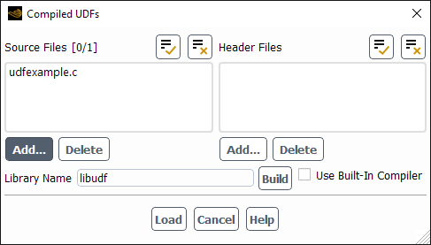
Controls
- Source Files
contains a list of source files.
- Header Files
contains a list of header files.
- Add...
opens the Select File dialog box.
- Delete
deletes the selected file from the list.
- Library Name
specifies the name of the library to be created.
- Use Built-In Compiler
enables the use of a built-in compiler (Clang) when the button is clicked. This option / compiler is available for Windows only, and is provided as part of the Fluent installation. It is recommended that you enable this option when the compiler you installed on your machine is older and no longer supported. Note that the built-in compiler is used automatically if Fluent determines that you have not installed Microsoft Visual Studio or Clang on your computer, whether this option is enabled or not.
- Build
builds the library and compiles the user-defined function.
- Load
opens the specified library and loads the user-defined function.
The Conduction Layers dialog box allows you to define the conduction settings for either a single Wall dialog box or all of the walls selected in the Wall Zones list of the Conduction Manager Dialog Box. See Shell Conduction and Managing Conduction Walls for details about the items below.
The Conduction Layers dialog box is opened from either the Wall Dialog Box or the Conduction Manager Dialog Box.
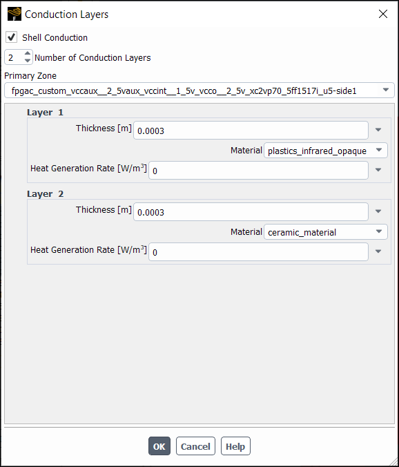
Controls
- Shell Conduction
enables/disables shell conduction for the selected wall(s).
- Number of Shell Conduction Layers
allows you to define the number of layers that make up the wall(s).
- Primary Zone
sets a wall to copy conduction settings from to the other selected walls.
- Layer 1, Layer 2...
allows you to define the settings for each layer. Note that Layer 1 refers to the layer closest to the fluid / solid adjacent to the wall zone, and layers with higher numbers are further away.
- Thickness
sets the thickness of the layer for the calculation of the thermal resistance. Each layer must have a nonzero thickness. Note that non-shell walls with a specified Thickness will be treated as thin walls.
- Material Name
sets the material type for the layer/wall. The conductivity of the material is used for the calculation of thermal resistance. Materials are defined using the Materials Task Page.
- Heat Generation Rate
sets the rate of heat generation in the layer. Note that you have the option of defining the heat generation rate using a user-defined function (UDF) that utilizes the
DEFINE_PROFILEmacro; for more information on creating and using user-defined functions, see the Fluent Customization Manual.
The Conduction Manager dialog box allows you to manage, define, and display conduction zones all in one location.
![]() Physics → Model Specific
→ Conduction Manager...
Physics → Model Specific
→ Conduction Manager...
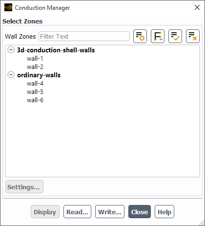
Controls
- Select Zones
contains the list of conduction zones (1d thin walls and 3d shell walls) and ordinary walls.
- Wall Zones
contains a list of wall zones.
- Settings...
opens the Conduction Layers Dialog Box, where you can define the conduction properties of the walls selected in the Wall Zones list.
- Display
displays the selected walls in the graphics window.
- Read...
allows you to define your conduction settings by reading a
.csvfile.- Write...
allows you to write your saved conduction settings to a
.csvfile.
The Contours dialog box controls the display of contour and profile plots. See Displaying Contours and Profiles for details about the items below.
![]() Results → Graphics
→ Contours → New...
Results → Graphics
→ Contours → New...
Note:
The "global"/non-persistent form of graphics objects is hidden by default. If this interrupts your workflow, you can make them available by enabling the Expose legacy non-persistent graphics option in the Graphics branch of Preferences (accessed via File>Preferences...).
(When you click Edit... instead of New..., it opens the "global"/non-persistent version of the Contours dialog box. This version of the dialog box does not have a Name field and it is not saved with the case file.
You are encouraged to use the persistent version that is accessed by clicking New....
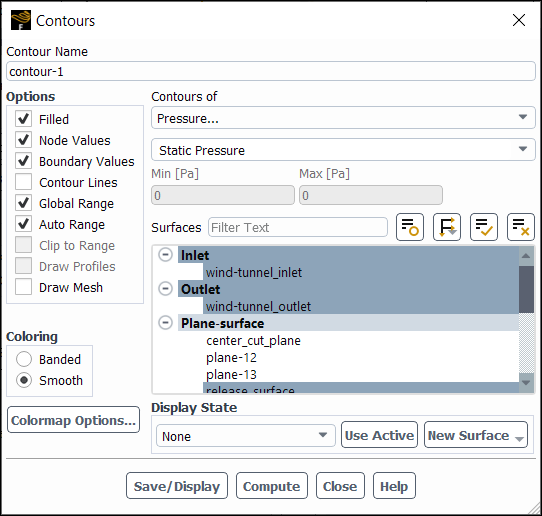
Controls
- Contour Name
is the name for a contour plot definition. You can specify a name or use the default name
contour-. This control appears only for contour plot definitions.id- Options
contains the check buttons that set various contour display options.
- Filled
toggles between filled contours and line contours.
- Node Values
toggles between using scalar field values at nodes and at cell centers for computing the contours. When the Filled option is off, Node Values is always on. See Choosing Node or Cell Values and Node or Boundary Values and Node Values for details.
- Boundary Values
enabling overwrites the node values (on boundaries) with a simple average of the boundary face values. Refer to Choosing Node or Cell Values and Node or Boundary Values for more information.
- Contour Lines
combines filled contours with line contours. This option is only available when both the Filled and Node Values options are enabled.
- Global Range
toggles between basing the minimum and maximum values on the range of values on the selected surfaces (off), and basing them on the range of values in the entire domain (on, the default).
- Auto Range
toggles between automatic and manual setting of the contour range. Any time you change the Contours of selection, Auto Range is reset to on.
- Clip to Range
determines whether or not values outside the prescribed Min/ Max range are contoured when using Filled contours. If selected, values outside the range will not be contoured. If not selected, values below the Min value will be colored with the lowest color on the color scale, and values above the Max value will be colored with the highest color on the color scale. See Specifying the Range of Magnitudes Displayed for details.
- Draw Profiles
causes the addition of a profile plot to the contour plot. The Profile Options Dialog Box is opened when Draw Profiles is selected.
Note: Draw Profiles is only available for the non-persistent/"global" version of the Contours dialog box that does not have a Name field. This version of the dialog box is opened by:
Right-clicking Contours in the Outline View tree and selecting Edit... (located under the Results branch).
Clicking Contours and selecting Edit... under Graphics in the Results ribbon tab.
- Draw Mesh
toggles between displaying and not displaying the mesh. The Mesh Display Dialog Box is opened when Draw Mesh is selected.
- Coloring
specifies how the contours appear.
- Banded
the contour coloring features distinct color bands corresponding to the colormap.
- Smooth
the contours feature a smooth transition between colors.
- Colormap Options...
opens the Colormap Dialog Box, allowing you to customize the colormap for this graphics object.
- Contours of
contains a list from which you can select the scalar field to be contoured.
- Min
shows the minimum value of the scalar field. If Auto Range is off, you can set the minimum by typing a new value.
- Max
shows the maximum value of the scalar field. If Auto Range is off, you can set the maximum by typing a new value.
- Surfaces
contains a list from which you can select the surfaces on which to draw contours. For 2D cases, if no surface is selected, contouring is done on the entire domain. For 3D cases, you must always select at least one surface.
- Display State
specifies the display state that is associated with this graphics object.
- drop-down list of display states
selectable list of all the existing display states associated with this case.
creates a display state that matches the settings of the active graphics window and assigns it to this graphics object (this association is only saved after you click ).
- New Surface
is a drop-down list button that contains a list of surface options:
- Point
opens the Point Surface Dialog Box.
- Line/Rake
opens the Line/Rake Surface Dialog Box.
- Plane
opens the Plane Surface Dialog Box.
- Quadric
opens the Quadric Surface Dialog Box.
- Iso-Surface
opens the Iso-Surface Dialog Box.
- Iso-Clip
opens the Iso-Clip Dialog Box.
- Structural Point
opens the Structural Point Surface Dialog Box.
- Display
draws the contours in the active graphics window.
- Compute
calculates the scalar field and updates the Min and Max values (even when Auto Range is off).
- Save/Display
plots the contour in the active graphics window and saves the contour plot definition. This button appears only for contour plot definitions and replaces the Display button.
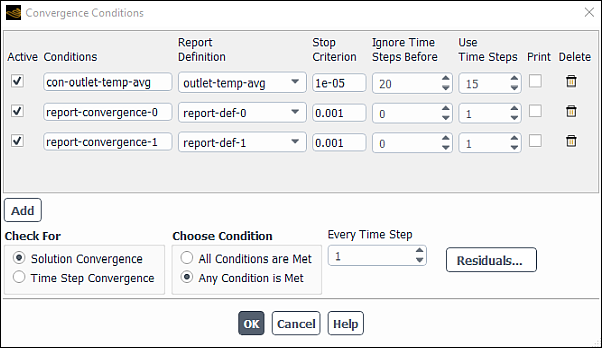
The convergence conditions facility allows you to set convergence conditions on the solution based on the values from report definitions (surface, volume, lift, drag, and so on). See Convergence Conditions for details on setting up the Convergence Conditions dialog box.
Note: If you are solving a transient case, the Convergence Conditions dialog box will relabel some fields since the transient case uses time-steps rather than iterations. These alternate labels are indicated below.
![]() Solution → Reports
→ Conditions...
Solution → Reports
→ Conditions...
Controls
- Active
check box for deactivating/activating individual convergence conditions.
- Conditions
name of the convergence condition.
- Report Definition
name of the report definition used in judging convergence.
- Stop Criterion
specifies the criterion below which the solution is considered to be converged.
- Ignore Iterations Before | Ignore Time Steps Before
ignores the first few iterations/time-steps if you expect the solution to fluctuate initially.
- Use Iterations | Use Time Steps
specifies the number of previous iterations/time-steps to be included in the report definition convergence check.
- Check For
specify whether Fluent checks for convergence at every time step or every iteration.
- Solution Convergence
Fluent checks for solution convergence at every time step.
- Time Step Convergence
Fluent checks for solution convergence at every iteration.
- Choose Condition
to select the convergence conditions.
- All Conditions are Met
The solution is considered to be converged if all of the convergence conditions’ criteria are satisfied, including those in the Residual Monitors Dialog Box.
- Any Condition is Met
The solution is considered to be converged if any of the convergence conditions’ criteria is satisfied, including those in the Residual Monitors Dialog Box.
- Every Iteration | Every Time-Step
to select how often convergence checks are done.
The Create Mesh Interfaces dialog box allows you to easily create many mesh interfaces between boundary zones that do not currently overlap (for example, for a sliding mesh simulation), as described in Manually Creating Many Non-Overlapping Mesh Interfaces. Note that if you only want to create mesh interfaces between boundary zones that currently overlap, you should instead use the Mesh Interfaces Dialog Box. For details, see Using a Non-Conformal Mesh in Ansys Fluent.
The Create Mesh Interfaces dialog box is opened by ensuring that
the default one-to-one interface creation method is enabled (using the
define/mesh-interfaces/one-to-one-pairing? text command) and
clicking the button in the Mesh Interfaces Dialog Box.
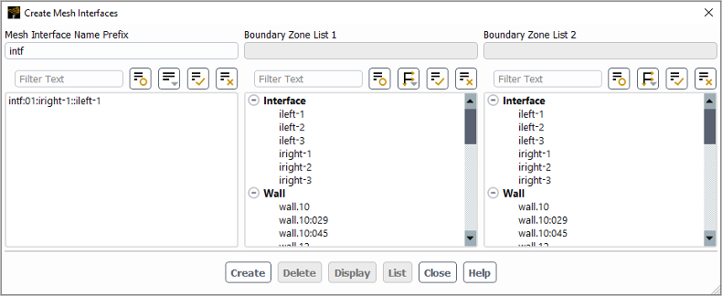
Controls
- Mesh Interface Name Prefix
contains a text entry box in which you can specify the prefix used in the names of all the mesh interfaces created when you click the button, and a list from which you can select existing mesh interfaces.
- Boundary Zone List 1, Boundary Zone List 2
allows you to select the zones that you want to pair up to make mesh interfaces. Note that mesh interfaces will be created for every possible combination between these two lists, regardless of whether the zones in question currently overlap. (You cannot edit the top fields; the names in these fields will be the name of the last zone you selected in the list below it.)
creates mesh interfaces for every possible combination between the zones selected under Boundary Zone List 1 and Boundary Zone List 2, regardless of whether the zones in question currently overlap.
deletes the mesh interfaces selected from the list under Mesh Interface Name Prefix.
allows you to display selected interface zones or mesh interfaces in the graphics window. Note that after you have selected a mesh interface, you can modify what zones are displayed by selecting / deselecting zones under Boundary Zone List 1 and/or Boundary Zone List 2.
prints information about the mesh interfaces selected in the list under Mesh Interface Name Prefix in the console.
The Create/Edit Mesh Interfaces dialog box allows you to manually create mesh interfaces for use with sliding meshes (see Using Sliding Meshes) or multiple reference frames (see Mesh Setup for a Multiple Moving Reference Frame), or for meshes with non-conformal boundaries (see Non-Conformal Meshes). This dialog box requires you to decide which interface zones make up both sides of each mesh interface. While it is possible to create every type of many-to-many mesh interface using this dialog box, it is only necessary when you want your interface to use the periodic or periodic repeats option; for all other types it is more convenient to automatically create interfaces using the Mesh Interfaces Dialog Box, especially when you have many interface zones and/or are unfamiliar with their names / locations. For details, see Using a Non-Conformal Mesh in Ansys Fluent.
The Create/Edit Mesh Interfaces dialog box
is opened by disabling the default one-to-one interface creation method (using the
define/mesh-interfaces/one-to-one-pairing? text command) and
clicking the button in the Mesh Interfaces Dialog Box.
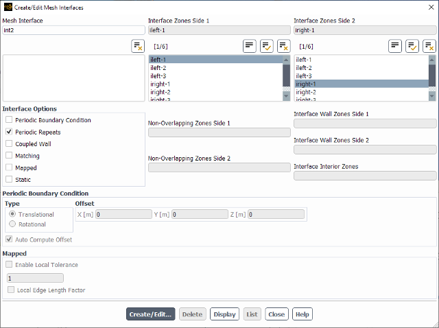
Controls
- Mesh Interface
contains a text entry box in which you can set the name of the mesh interface, and a list from which you can select an existing mesh interface.
- Interface Zones Side 1, Interface Zones Side 2
contain selectable lists for the interface zones that make up the mesh interface and informational fields that show the names of the zones you selected in each list. (You cannot edit the top fields; the names in these fields will be the names of the zones you selected in the list below it.)
- Interface Options
contains options related to the interface type.
- Periodic Boundary Condition
allows you to create a non-conformal periodic boundary condition interface. Note that the Matching option is enabled by default with such periodic mesh interfaces.
- Periodic Repeats
should be enabled when each of the two cell zones has a single pair of conformal or non-conformal periodics adjacent to the interface. This option is typically used in conjunction with the sliding mesh model, when simulating the interface between a rotor and stator; it allows Ansys Fluent to treat the interface between the sliding and non-sliding zones as periodic where the two zones do not overlap. For details, see The Periodic Repeats Option.
- Coupled Wall
allows you to specify that the interface acts as a thermally coupled wall.
- Matching
is relevant if only interface internal zones should be created (that is, interior or wall / shadow pairs), since the interface zones on both sides are aligned. With the Matching option, even interface zones that are not perfectly aligned are treated as if they are; however, if the discrepancy between the interface zones on both sides exceeds default thresholds, then warning messages will be displayed. Note that the Matching option is compatible with the Periodic Boundary Condition, Coupled Wall, and Static options. For more information about the recommended uses of this option, see Matching Option.
- Mapped
enables an alternative approach for modeling coupled walls between zones. This approach is more robust than the standard non-conformal interface formulations when the interface zones penetrate each other or have gaps between them. It requires that at least one side of the interface consists of only solid zones.
Note: The Mapped option is not compatible with shell conduction.
- Static
reduces the memory usage and processing time (for interface creation and solution), especially when there are many zones on both sides of the interface. This option will only produce correct results if the interface zones do not move or deform relative to each other at the interface, and it is not compatible with the Periodic Boundary Condition, Periodic Repeats, or Mapped options.
- Non-Overlapping Zones Side 1, Non-Overlapping Zones Side 2
display the names of any wall boundary zones created by Ansys Fluent during the process of creating the selected mesh interface. If the two interface zones overlap each other completely, then the wall boundaries are created but with zero faces.
- Interface Wall Zones Side 1, Interface Wall Zones Side 2
display the names of any wall interface zones created by Ansys Fluent during the process of creating the selected mesh interface.
- Interface Interior Zones
displays the names of any interface interior zones created by Ansys Fluent during the process of creating the selected mesh interface. This is used for embedded LES, when there is a need to be able to convert an interior zone into a RANS-LES interface.
- Periodic Boundary Condition
- Type
allows you to select a periodicity that is either Translational or Rotational.
- Offset
is the offset coordinates or angle, depending on whether Translational or Rotational periodicity is selected. Note that when Auto Compute Offset is enabled, the Offset fields are not editable.
- Auto Compute Offset
will result in Ansys Fluent finding the offset. If this option is disabled, then you will have to provide the offset coordinates or angle in the required fields, depending on whether Translational or Rotational periodicity is selected.
- Mapped
- Enable Local Tolerance
(when enabled) allows you to overwrite any value specified in the Tolerance group box in the Mapped Interface Options Dialog Box, and is used on the selected interface only.
- Local Edge Length Factor
(when enabled) allows you to specify the multiplier that Fluent uses with the smallest edge length of the interface zones to calculate the tolerance for mapping. Disabling Local Edge Length Factor allows you to specify an absolute value for the tolerance.
performs one of the following:
If you have entered a new Mesh Interface name and selected unassigned zones from the Interface Zones Side 1 and Interface Zones Side 2 selection lists, a new mesh interface is created.
If you have made a selection from the Mesh Interface list, the Edit Mesh Interfaces Dialog Box will open so that you can revise the settings of existing mesh interfaces.
deletes the mesh interface selected under Mesh Interface.
allows you to display interface zones or mesh interfaces in the graphics window. Note that you can only select and display an interface zone from Interface Zones Side 1 or Interface Zones Side 2 if it is not yet assigned to an existing mesh interface. After a Mesh Interface is created, you can select the appropriate mesh interface and click the button to display all of the zones under Interface Zones Side 1 and Interface Zones Side 2.
prints information about the selected Mesh Interface in the console. When you click this button, Ansys Fluent will list the two interface boundaries and (if you have initialized the solution) all new zones that were created (that is, wall and/or interior zones).
The Create/Edit Turbo Interfaces dialog box allows you to manually create many-to-many mesh interfaces to connect blades to one another. This dialog box requires you to decide which interface zones make up both sides of each turbo interface and specify the blade row interaction model. For details, see Creating and Editing General Turbo Interfaces.
Controls
- Mesh Interface
contains a text entry box in which you can set the name of the turbo interface, and a list from which you can select an existing mesh interface.
- Interface Zones Side 1, Interface Zones Side 2
contain selectable lists for the interface zones that make up the turbo interface and informational fields that show the names of the zones you selected in each list. (You cannot edit the top fields; the names in these fields will be the names of the zones you selected in the list below it.)
- Interface Options
contains options related to the interface type.
- Periodic Boundary Condition
allows you to create a non-conformal periodic boundary condition interface. Note that the Matching option is enabled by default with such periodic mesh interfaces; for details about the Matching option, see Matching Option.
- General Turbo Interface
(only available when the Turbo Model is enabled) connects two turbo zones. This option is typically used in conjunction with the sliding mesh model, when simulating the interface between a rotor and stator. These models permit for a pitch-change between the modeled blade rows.
- Pitch-Change Types
- Pitch-Scale
stretches or compresses the flow profiles between the cell zones to maintain the interaction between blade row passages. See Blade Row Interaction Modeling for details.
- No Pitch-Scale
maintains the blade row interaction between blade row passages by creating virtual copies of the smaller pitch blade passage. See Blade Row Interaction Modeling for details.
- Mixing Plane
uses a pitchwise averaging procedure to mix out the flow variation between the blade rows. See Blade Row Interaction Modeling for details.
performs one of the following:
If you have entered a new Mesh Interface name and selected unassigned zones from the Interface Zones Side 1 and Interface Zones Side 2 selection lists, a new mesh interface is created.
If you have made a selection from the Mesh Interface list, the Edit Mesh Interfaces Dialog Box will open so that you can revise the settings of existing mesh interfaces.
deletes the mesh interface selected under Mesh Interface.
allows you to display interface zones or mesh interfaces in the graphics window. Note that you can only select and display an interface zone from Interface Zones Side 1 or Interface Zones Side 2 if it is not yet assigned to an existing mesh interface. After a Mesh Interface is created, you can select the appropriate mesh interface and click the button to display all of the zones under Interface Zones Side 1 and Interface Zones Side 2.
prints information about the selected Mesh Interface in the console. When you click this button, Ansys Fluent will list the two interface boundaries and (if you have initialized the solution) all new zones that were created (that is, wall and/or interior zones).
The Curvilinear Coordinate System dialog box allows you to create local coordinate systems that follow the geometry of the model. Refer to Curvilinear Coordinate Systems for additional information.
Controls
- Name
specifies the name of the curvilinear coordinate system.
specifies the cell zone whose geometry will be used to create the curvilinear coordinate system.
- Direction 0 (1)
tabs to specify Direction 0 and 1 of the curvilinear coordinate system. Note that Direction 2 is calculated from the cross product of Direction 0 and 1.
There are 2 options for specifying a direction.
Diffusion - utilizes geometry to specify direction as determined by Boundary Specification.
- Start and End
specifies the direction using a Start Face Zone and an End Face Zone.
- Jump
for closed loop geometries, specifies the direction from Interior Zones (utilizing a coupled wall as a cross section, which is then split into start and end faces).
Base Vector - specifies the direction using an X, Y, Z vector
- Display Face Zones
displays currently selected face zones.
options to visualize the curvilinear coordinate system.
- Direction 0
selects Direction 0 to display in the graphics viewer.
- Direction 1
selects Direction 1 to display in the graphics viewer.
- Direction 2
selects Direction 2 to display in the graphics viewer.
- Auto Scale
scales the vectors to an appropriate size.
- Draw Mesh
opens the Mesh Display dialog box.
- Scale
specifies the size of the vectors for display.
- Skip
Thins the number of vectors displayed to improve visibility.
- Save
Saves the curvilinear coordinate system.
- Display
Displays the curvilinear coordinate system according the settings under .
The Custom Field Function Calculator dialog box allows you to define custom field functions based on existing functions, using simple calculator operators. Any functions that you define will be added to the list of default flow variables and other field functions provided by Ansys Fluent.
Important: Recall that you must enter all constants in the function definition in SI units.
See Creating a Custom Field Function for details about the items below.
![]() User Defined → Field Functions
→ Custom...
User Defined → Field Functions
→ Custom...
Controls
- Definition
displays the function that you are currently defining. As you select each item from the Field Functions list or the calculator keypad, it will appear in the Definition text entry box. You cannot edit the contents of this box directly; if you want to delete part of a function, use the button on the keypad.
- (Calculator Buttons)
are buttons that perform calculator operations. When you select a calculator button (by clicking on it), the appropriate symbol will appear in the Definition text entry box.
- Select Operand Field Functions from
contains the available field functions and the means for selecting them.
- Field Functions
contains a list from which you can select a variable to be used in the definition of a new function.
- Select
enters the variable that is currently selected in the Field Functions list in the Definition field.
- New Function Name
specifies the name of the function you are defining. Should you decide to change the function name after you have defined the function, you can do so in the Field Function Definitions Dialog Box, which you can open by clicking on the Manage... button.
creates the function and adds it to the list of Custom Field Functions within the drop-down list of available field functions. The button is grayed out after you create a new function or if the Definition field is empty.
- Manage...
opens the Field Function Definitions Dialog Box, which enables you to check, rename, save, load, and delete custom field functions.
The Custom Laws dialog box is used to incorporate user-defined functions (see the separate Fluent Customization Manual for details) in place of the default physical laws used in the heat/mass transfer calculations.
The Custom Laws dialog box is opened from the Set Injection Properties Dialog Box.
Controls
- First Law, Second Law, Third Law,...
contain drop-down lists in which you can choose a user-defined particle law to replace the standard law.
- Switching
contains a drop-down list in which you can select a user-defined function that customizes the way Ansys Fluent switches between particle laws.
The Dashboard Definition dialog box allows you create custom embedded window dashboards that are saved with the case file and added to the Outline View tree. See Geometry-Based Adaption with the Hanging Node Method for details.
![]() Results → Graphics
→ Dashboard...
Results → Graphics
→ Dashboard...
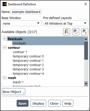
Controls
- Name
is the name for a dashboard definition. You can specify a name or use the default name
dashboard-.id- Base Window
specifies which window will be the background, upon which all other graphics and plot objects are embedded. You can also leave it set to none, allowing you to arrange the child windows without any overlap.
- Pre-defined Layouts
controls how the embedded windows are arranged when they are displayed first displayed. You can manually move and resize the windows once they are displayed.
- Available Objects
lists the available graphics and plot objects that can be included in the dashboard.
- New Object
drop-down list allowing you to create additional graphics objects that can be included in the dashboard.
saves the dashboard to the case file.
saves the dashboard and displays it in the graphics window.
The Deactivate Cell Zones dialog box allows you to deactivate a single cell zone or multiple zones. See Deactivating Zones for details.
![]() Domain → Zones
→ Deactivate...
Domain → Zones
→ Deactivate...
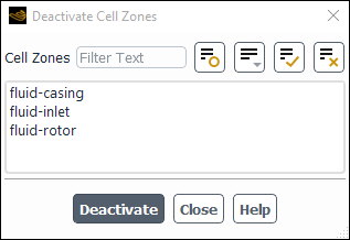
Controls
- Cell Zones
contains a list of cell zones from which you can select the zone to be deactivated.
- Deactivate
deactivates the selected cell zones.
The Define Control Points dialog box allows you to create, modify, and delete control points for the mesh morpher/optimizer when the unstructured control point distribution is selected. See Using the Mesh Morpher/Optimizer for details about using this dialog box.
The Define Control Points dialog box is opened from the Mesh Morpher/Optimizer Dialog Box.
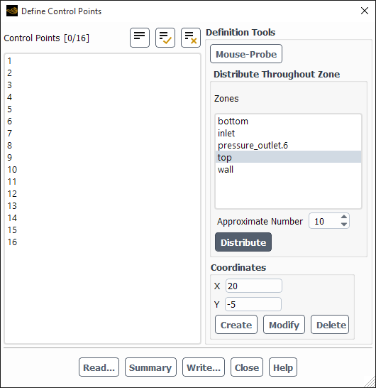
Controls
- Control Points
lists the control points you have created and allows you to modify and delete them.
- Definition Tools
provides tools for defining the control points.
- Mouse-Probe
allows you to create control points by probing (using the right mouse button, by default) in the graphics window.
- Distribute Throughout Zone
allows you to quickly create a number of control points and distribute them on mesh nodes throughout a specific boundary zone.
- Zones
allows you to select the boundary zone throughout which you want to distribute control points.
- Approximate Number
allows you to specify the approximate number of control points you want to distribute throughout a zone. Note that due to the method by which the control points are distributed, the actual number may exceed the value you enter.
- Distribute
creates a number of control points on mesh nodes throughout the specified zone (within the bounding box) with a distribution that is based on the distribution of the cell faces in that zone.
- Coordinates
allows you to view and modify the coordinates of control points, as well as to create new control points and to delete existing control points.
- X, Y, Z
displays the coordinates of the selected Control Point, and allows you to define new ones and edit existing ones.
- Create
creates a new control point at the currently displayed X, Y, and Z coordinates.
- Modify
revises the X, Y, and Z coordinates of the selected Control Point.
- Delete
deletes the selected Control Point.
The Delete Cell Zones dialog box allows you to delete a single cell zone or multiple zones. See Deleting Zones for details.
![]() Domain → Zones
→ Delete...
Domain → Zones
→ Delete...
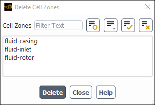
Controls
- Cell Zones
contains a list of cell zones from which you can select the zone to be deleted.
- Delete
deletes the selected cell zones.
The Display Options - Adaption dialog box allows you to customize how the cells marked for adaption are displayed.
This dialog box is accessed by clicking in the Manual Mesh Adaption Dialog Box or Automatic Mesh Adaption Dialog Box.
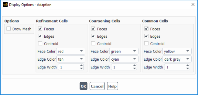
Controls
- Options
contains check boxes that controls the drawing of the mesh.
- Draw Mesh
toggles the ability to draw the mesh with the adaption display. This command opens the Mesh Display Dialog Box, which allows you to select the desired surface or zone meshes to be displayed with the markings.
- Refinement Cells
contains options related to the display of cells marked for refinement.
- Faces
controls whether cell faces are displayed on the cells marked for refinement.
- Edges
controls whether cell edges are displayed on the cells marked for refinement.
- Centroid
controls whether the cell centroid is displayed on the cells marked for refinement.
- Face Color
controls the color of the cell faces on the cells marked for refinement.
- Edge Color
controls the color of the cell edges on the cells marked for refinement.
- Edge Width
controls the thickness of the cell edges on the cells marked for refinement.
- Coarsening Cells
contains options related to the display of cells marked for coarsening.
- Faces
controls whether cell faces are displayed on the cells marked for coarsening.
- Edges
controls whether cell edges are displayed on the cells marked for coarsening.
- Centroid
controls whether the cell centroid is displayed on the cells marked for coarsening.
- Face Color
controls the color of the cell faces on the cells marked for coarsening.
- Edge Color
controls the color of the cell edges on the cells marked for coarsening.
- Edge Width
controls the thickness of the cell edges on the cells marked for coarsening.
- Common Cells
contains options related to the display of cells marked for both refinement and coarsening.
- Faces
controls whether cell faces are displayed on the cells marked for both refinement and coarsening.
- Edges
controls whether cell edges are displayed on the cells marked for both refinement and coarsening.
- Centroid
controls whether the cell centroid is displayed on the cells marked for both refinement and coarsening.
- Face Color
controls the color of the cell faces on the cells marked for both refinement and coarsening.
- Edge Color
controls the color of the cell edges on the cells marked for both refinement and coarsening.
- Edge Width
controls the thickness of the cell edges on the cells marked for both refinement and coarsening.
This dialog box is accessed by clicking in the View ribbon tab.
![]() View → Display
→ Display States...
View → Display
→ Display States...
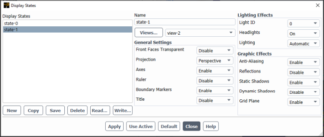
Controls
- Display States
single selection listing of all defined display states.
create a new display state with the same settings as the active graphics window (or the last active user window if the current active window is displaying a 2D plot).
create a new display state the copies the properties of the selected display state.
save the properties of the selected display state.
delete the selected state.
read in display states from a file.
write display states to a file.
- Name
name of the selected display state.
- Views...
opens the Views Dialog Box.
- Views Drop-down List
list of views that can be associated with this display state.
- General Settings
lists general graphics window settings.
- Front Faces Transparency
controls whether the front faces are transparent.
- Projection
specifies whether the display is in a perspective or orthographic view.
- Axes
controls whether or not the axes triad is displayed.
- Ruler
controls whether or not the ruler is displayed.
- Boundary Markers
controls whether or not boundary markers are displayed. Note that boundary markers are only displayed on mesh, not other graphics objects like contours or vectors.
- Title
controls whether or not the titles bar is displayed.
- Edge Color
controls the color of the cell edges on the cells marked for refinement.
- Lighting Effects
lists lighting settings.
- Light ID
controls which light ID is saved. If more than one light ID is active when you click Use Active from a graphics object dialog box, this option is set to Don't Save.
- Headlights
controls whether the headlight is on or off.
- Lighting
specifies the lighting method that is used for the display.
- Graphic Effects
lists the graphics effects.
- Anti-Aliasing
controls whether or not lines and text are smooth.
- Reflections
controls whether or not a reflection of the model is shown (with the axis of reflection being controlled in Preferences).
- Static Shadows
controls whether or not static shadows are displayed.
- Dynamic Shadows
controls whether or not dynamic shadows are displayed. These shadows move as you rotate your model and are computationally expensive to render.
- Grid Plane
controls whether or not the grid plane is shown (with the axis for the grid being controlled in Preferences).
save the settings of the selected display state and apply these settings to the active graphics window display.
update the currently-selected display state to inherit the display state settings of the active graphics window. This button is not available if the active graphics window is displaying a 2D plot.
resets the selected display state to match the default settings.
Table 52.1: Default Display State Settings
Setting State View isometric Front Faces Transparent Disable Projection Perspective Axes Enable Ruler Disable Boundary Markers Enable Title Disable Light ID 0 Headlights On Lighting Automatic Anti-Aliasing Enable Reflections Enable Static Shadows Enable Dynamic Shadows Disable Grid Plane Enable Note: The default graphics effects settings are dependent on the available graphics driver. If no modern graphics driver is available, graphics effects will be disabled.
![]() Solution → Reports
→ Definitions → New
→ DPM Report
Solution → Reports
→ Definitions → New
→ DPM Report
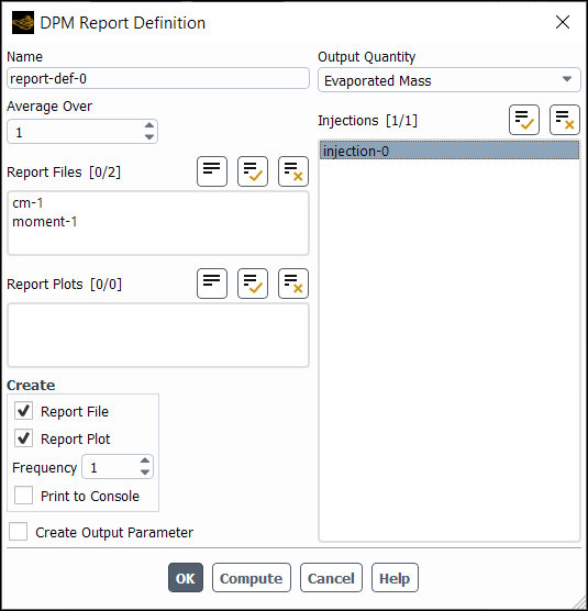
Controls
- Name
specifies the name of the report definition.
- Average Over
(optional) To have Fluent calculate a running average for the DPM Report Definition you can enter a positive integer greater than 1 (the default) for Average Over.
Specifying a number greater than 1 means that Fluent will print, plot, and write the running average value of the selected variable instead of the current value of the same variable.
The value reported is averaged over the last
 iterations/time steps, where
  is your specified Average Over value. When
the iteration/time step number is lower than
is your specified Average Over value. When
the iteration/time step number is lower than  , Fluent calculates the average of the available variable
values.
, Fluent calculates the average of the available variable
values.
- Retain Instantaneous Values
appears when Average Over is set to a value greater than
1. If enabled when you are creating a new report definition, it ensures that all instantaneous values are saved in the new report file that is being created for this report definition. It also results in the Plot Instantaneous Values option being enabled in the newly created report plot.- Report Files
lists all of the report files where you can write the report definition data.
- Report Plots
lists all of the report plots where you can plot the report definition data (assuming this report has the same units as the other report definitions included in the selected report plot).
- Create
options you can choose when creating your report.
- Report File
creates a new report file that includes this report definition.
- Report Plot
creates a new report plot that includes this report definition.
- Frequency
specifies how frequently the report definition is written, plotted, or printed to the console.
- Print to Console
prints the value of the report definition to the console.
- Create Output Parameter
creates an output parameter for this report definition with the name
<report definition name>-op.- Output Quantity
quantities that can be applied to the output parameter.
- Injected Mass
(unsteady particle tracking only) reports the total DPM mass injected into the domain.
- Mass in Domain
(unsteady particle tracking only) reports the total DPM mass present in the domain.
- Mass in Fluid
(unsteady particle tracking only) reports all DPM mass currently residing as free-stream particles in the domain. This option is available only with the wall-film DPM boundary condition.
- Mass in Film
(unsteady particle tracking only) reports all DPM mass currently residing in Lagrangian wall-film. This option is available only with the wall-film DPM boundary condition.
- Escaped Mass
reports the DPM mass that has left the domain through a certain boundary or boundaries.
- Evaporated Mass
reports the total evaporated DPM mass for the selected injection(s). The quantity accounts for fully evaporated particles as well as all mass that has evaporated from any other particles. For unsteady tracking, this includes particles that are still present in the domain.
- Penetration Length
(unsteady particle tracking only) reports the total penetration length in meters.
- Injections
lists the injections that you can select for discrete phase reporting. For the Escaped Mass output quantity, this item is available only if you have enabled the
report/dpm-zone-summaries-per-injectiontext command. Note that for unsteady particle tracking, if you want to report the mass of escaped particles per injection, this text command must be enabled before any particles are injected into the domain.- Boundaries
contains a selectable list of valid boundary zones for escaped mass reporting.
- Show Mass Flow/Change Rate
(unsteady particle tracking only) if enabled, specifies that the mass flow rate will be reported (default). Otherwise the total mass will be reported. This item is not available for the Penetration Length report.
- Particles Mass Fraction
the mass fraction expected between the injection nozzle and the penetration length. This item is available only for the Penetration Length reports.
- User-Specified Origin and Direction
once enabled, it allows you to specify the Origin and Direction of the selected injection(s). This item is available only for the Penetration Length reports.
- OK
creates the report definition.
- Compute
computes the value of the report definition and prints to the console.
![]() Solution → Reports
→ Definitions → New
→ Flux Report → DPM Mass Source | DPM
Enthalpy Source | DPM Sensible Enthapy Source
Solution → Reports
→ Definitions → New
→ Flux Report → DPM Mass Source | DPM
Enthalpy Source | DPM Sensible Enthapy Source
Controls
- Name
specifies the name of the report definition.
- Function
functions available for the source report definition.
- DPM Mass Source
reports the mass contributions from the particle injections.
- DPM Enthalpy Source
reports the heat contributions from the particle injections.
- DPM Sensible Enthalpy Source
reports the sensible heat contributions from the particle injections.
- Average Over
(optional) To have Fluent calculate a running average for the DPM Source Report Definition you can enter a positive integer greater than 1 (the default) for Average Over.
Specifying a number greater than 1 means that Fluent will print, plot, and write the running average value of the selected variable instead of the current value of the same variable.
The value reported is averaged over the last
iterations/time steps, where is your specified Average Over value. When
the iteration/time step number is lower than , Fluent calculates the average of the available variable
values.
- Retain Instantaneous Values
appears when Average Over is set to a value greater than
1. If enabled when you are creating a new report definition, it ensures that all instantaneous values are saved in the new report file that is being created for this report definition. It also results in the Plot Instantaneous Values option being enabled in the newly created report plot.- Report Files
lists all of the report files where you can write the report definition data.
- Report Plots
lists all of the report plots where you can plot the report definition data (assuming this report has the same units as the other report definitions included in the selected report plot).
- Create Output Parameter
creates an output parameter for this report definition with the name
<report definition name>-op.- Create
options you can choose while generating a report.
- Report File
creates a new report file that includes this report definition.
- Report Plot
creates a new report plot that includes this report definition.
- Frequency
specifies how frequently the report definition is written, plotted, or printed to the console.
- Print to Console
prints the value of the report definition to the console.
- Compute
computes the value of the report definition and prints to the console.
- OK
creates the report definition.
![]() Solution → Reports
→ Definitions → New
→ Force Report → Drag...
Solution → Reports
→ Definitions → New
→ Force Report → Drag...
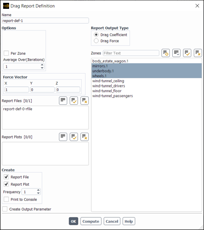
Controls
- Name
specifies the name of the report definition.
- Options
options you can choose for the drag report.
- Per Zone
specifies whether or not the drag for multiple walls zones should be monitored on each wall zone separately. When this option is turned off (the default), Fluent computes and monitors the total drag for all of the selected walls zones combined together.
- Average Over (Time-Steps), Average Over (Iterations)
(optional) To have Fluent calculate a running average for the Drag Report Definition you can enter a positive integer greater than 1 (the default) for Average Over.
Specifying a number greater than 1 means that Fluent will print, plot, and write the running average value of the selected variable instead of the current value of the same variable.
The value reported is averaged over the last
iterations/time steps, where is your specified Average Over value.
When the iteration/time step number is lower than , Fluent calculates the average of the available variable
values.
- Retain Instantaneous Values
appears when Average Over is set to a value greater than
1. If enabled when you are creating a new report definition, it ensures that all instantaneous values are saved in the new report file that is being created for this report definition. It also results in the Plot Instantaneous Values option being enabled in the newly created report plot.- Force Vector
contains the components of the force vector.
- X,Y,Z
are the components of the force vector along which the forces will be computed.
- Report Files
lists all of the report files where you can write the report definition data.
- Report Plots
lists all of the report plots where you can plot the report definition data (assuming this report has the same units as the other report definitions included in the selected report plot).
- Create
options you can choose while generating a report.
- Report File
creates a new report file that includes this report definition.
- Report Plot
creates a new report plot that includes this report definition.
- Frequency
specifies how frequently the report definition is written, plotted, or printed to the console.
- Print to Console
prints the value of the report definition to the console.
- Create Output Parameter
creates an output parameter for this report definition with the name
<report definition name>-op.- Report Output Type
options you can choose relevant to report output.
- Drag Coefficient
specifies the report definition as a unitless quantity.
- Drag Force
specifies that the report definition has units of force.
- Zones
lists the zones you can select for drag coefficient or drag force computation.
- OK
creates the report definition.
- Compute
computes the value of the report definition at the selected zone(s) and prints to the console.
The DTRM Graphics dialog box allows you to display rays and clusters used by the DTRM. See Displaying Rays and Clusters for the DTRM for details.
![]() Results → Model Specific
→ DTRM Graphics...
Results → Model Specific
→ DTRM Graphics...
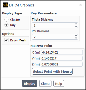
Controls
- Display Type
contains options for the different items you can display.
- Cluster
specifies the display of clusters.
- Ray
specifies the display of rays.
- Options
contains check buttons that control display options.
- Draw Mesh
toggles between displaying and not displaying the mesh. The Mesh Display Dialog Box is opened when Draw Mesh is selected.
- Cluster Type
specifies whether Surface clusters or Volume clusters are to be displayed. This section of the dialog box appears when Cluster is selected as the Display Type.
- Cluster Selection
contains options for cluster displays. This section of the dialog box appears when Cluster is selected as the Display Type.
- Display All Clusters
enables the display of all surface or volume clusters in the domain.
- Ray Parameters
contains controls for displaying rays. This section of the dialog box appears when Ray is selected as the Display Type.
- Theta Divisions, Phi Divisions
control the number of rays being traced. (See Controlling the Rays.)
- Nearest Point
specifies a point (X,Y,Z) near the cluster to be displayed (or the cluster from which the rays should start).
The Nearest Point controls are not available when Display All Clusters is selected under Cluster Selection.
- Select Point With Mouse
is an alternative method for specifying the Nearest Point using your mouse, by clicking the button.
- Display
displays the specified cluster(s) or rays.
The DTRM Rays dialog box allows you to define the rays used by the discrete transfer radiation model (DTRM). It opens automatically when you click after selecting the Discrete Transfer model in the Radiation Model Dialog Box. See Setting Up the DTRM for details about the items below.
![]() Physics → Model Specific
→ DTRM Rays...
Physics → Model Specific
→ DTRM Rays...
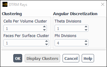
Controls
- Clustering
contains parameters for the clusters (see Clustering in the Theory Guide).
- Cells Per Volume Cluster, Faces Per Surface Cluster
control the number of radiating surfaces and absorbing cells. (See the explanation in Controlling the Clusters.)
- Angular Discretization
contains parameters for the ray traces (see Ray Tracing in the Theory Guide).
- Theta Divisions, Phi Divisions
control the number of rays being traced. (Guidelines are provided in Controlling the Rays.)
- Display Clusters
generates a graphical display of the clusters in the domain. (This item is available only after you have created or read a ray file.)
The Edit Gap Region dialog box allows you to edit an existing gap region as part of a gap model simulation. It is opened by making a selection from the Gap Regions list in the Gap Model Dialog Box and clicking . See also Controlling Flow in Narrow Gaps for Valves and Pumps.
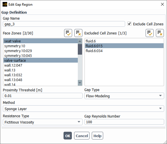
Controls
- Gap Definition
contains input controls for editing an existing gap region.
- Gap Name
specifies the name of the gap region. It cannot consist solely of numbers.
- Face Zones
allows you to select the two or more face zones that constitute the gap region.
- Proximity Threshold
defines the maximum distance between the face zones when flow blockage / deceleration occurs in the gap.
- Gap Type
defines the type of the gap region. A Flow-Blocking type completely blocks the flow in the gap region, as a numerical zero-mass-flux boundary condition is applied at the boundary faces of the marked region so that the marked cells no longer participate in the solution. A Flow-Modeling type decelerates the flow in the cells of the marked region by manipulating the viscosity or source terms.
- Method
defines the method used to scale the viscosity or to define source terms in the gap region. The Sponge Layer method specifies that the viscosity inside the gap regions is scaled based on the specified Gap Reynolds Number. The User-Defined Source method specifies the use of a compiled user-defined function (UDF) to define the source terms for the momentum and energy equations in the gap region. This drop-down list is only available when Flow-Modeling is selected for the Gap Type.
- Resistance Type
specifies how the viscosity is scaled in the gap region. The Fictitious Viscosity approach scales the laminar viscosity inside the gap region during discretization of the viscous forces for the momentum equation; thus, its impact is explicitly seen in the velocity and pressure computation, and it has an implicit effect on the other solution fields through the changes in the velocity and pressure field. The Real Viscosity approach changes the actual laminar viscosity inside the gap region based on your specified Gap Reynolds Number; therefore, the effect of modeling will be seen not only in flow equation but also in other equations. This drop-down list is only available when Flow-Modeling is selected for the Gap Type and Sponge Layer is selected for the Method.
- Gap Reynolds Number
defines the intended Reynolds number in the gap region, and thus determines the level of sealing. A lower Gap Reynolds Number results in better sealing. It can be estimated according to Equation 6–4. This drop-down list is only available when Flow-Modeling is selected for the Gap Type and Sponge Layer is selected for the Method.
- Gap Source Terms
selects a compiled user-defined function (UDF) that specifies the source terms for the momentum and energy equations in the gap region using the
DEFINE_GAP_MODEL_SOURCEmacro. This drop-down list is only available when Flow-Modeling is selected for the Gap Type and User-Defined Source is selected for the Method.- Exclude Cell Zones
enables the ability to specify that cells in particular cell zones are not marked for flow blockage / deceleration as part of the gap region, in order to have greater control over the shape of the gap region.
- Excluded Cell Zones
selects the cell zones in which cells are not marked for flow blockage / deceleration as part of the gap region.
The Edit Mesh Interfaces dialog box allows you to edit existing many-to-many mesh interfaces. It is opened by making a selection from the Mesh Interfaces list in the Mesh Interfaces Dialog Box and clicking . See also Using a Non-Conformal Mesh in Ansys Fluent.
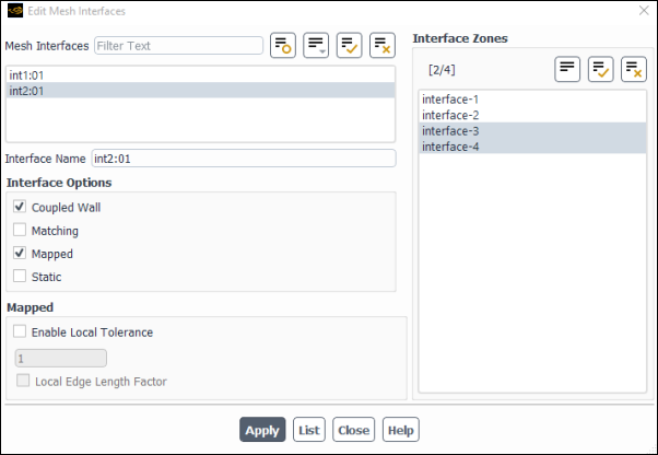
Controls
- Mesh Interfaces
allows you to select the mesh interfaces you would like to edit. Note that you can click the
 button to group the interfaces in the list by their currently
enabled interface option(s), which allows you to select / deselect all those of a
particular type by simply clicking the top-level branch.
button to group the interfaces in the list by their currently
enabled interface option(s), which allows you to select / deselect all those of a
particular type by simply clicking the top-level branch. - Interface Name
edits the name of the mesh interface. This is only available when a single interface is selected.
- Interface Options
contains options related to the interface type. These options can be applied when a single or multiple interfaces are selected.
- Periodic Boundary Condition
allows you to create a non-conformal periodic boundary condition interface.
- Periodic Repeats
should be enabled when each of the two cell zones has a single pair of conformal or non-conformal periodics adjacent to the interface. This option is typically used in conjunction with the sliding mesh model, when simulating the interface between a rotor and stator; it allows Ansys Fluent to treat the interface between the sliding and non-sliding zones as periodic where the two zones do not overlap. For details, see The Periodic Repeats Option.
- Coupled Wall
allows you to specify that the interface acts as a thermally coupled wall.
- Matching
is relevant if only interface internal zones should be created (that is, interior or wall / shadow pairs), since the interface zones on both sides are aligned. With the Matching option, even interface zones that are not perfectly aligned are treated as if they are; however, if the discrepancy between the interface zones on both sides exceeds default thresholds, then warning messages will be displayed. Note that the Matching option is compatible with the Periodic Boundary Condition, Coupled Wall, and Static options. For more information about the recommended uses of this option, see Matching Option.
- Mapped
enables an alternative approach for modeling coupled walls between zones. This approach is more robust than the standard non-conformal interface formulations when the interface zones penetrate each other or have gaps between them. It requires that at least one side of the interface consists of only solid zones.
Note: The Mapped option is not compatible with shell conduction.
- Static
reduces the memory usage and processing time (for interface creation and solution), especially when there are many zones on both sides of the interface. This option will only produce correct results if the interface zones do not move or deform relative to each other at the interface, and it is not compatible with the Periodic Boundary Condition, Periodic Repeats, or Mapped options.
- Periodic Boundary Conditions
- Type
allows you to select a periodicity that is either Translational or Rotational.
- Offset
is the offset coordinates or angle, depending on whether Translational or Rotational periodicity is selected. Note that when Auto Compute Offset is enabled, the Offset fields are not editable.
- Auto Compute Offset
will result in Ansys Fluent finding the offset. If this option is disabled, then you will have to provide the offset coordinates or angle in the required fields, depending on whether Translational or Rotational periodicity is selected.
- Mapped
- Enable Local Tolerance
(when enabled) allows you to overwrite any value specified in the Tolerance group box in the Mapped Interface Options Dialog Box, and is applied to the selected interface only.
- Local Edge Length Factor
(when enabled) allows you to specify the multiplier that Fluent uses with the smallest edge length of the interface zones to calculate the tolerance for mapping. Disabling Local Edge Length Factor allows you to specify an absolute value for the tolerance.
- Interface Zones
highlights the list of interface zones that make up the selected mesh interface and allows you to edit the list (provided that the zones you select are unassigned and located appropriately). This functionality is only available when a single interface is selected.
prints information in the console about the first mesh interface you selected. When you click this button, Ansys Fluent will list the interface boundaries and (if you have initialized the solution) all new zones that were created (that is, wall and interior zones).
saves the revised settings for the selected mesh interfaces.
![]() Solution → Reports
→ File...
Solution → Reports
→ File...
Select a report file in the Report File Definition dialog box and click to open the Edit Report File dialog box.
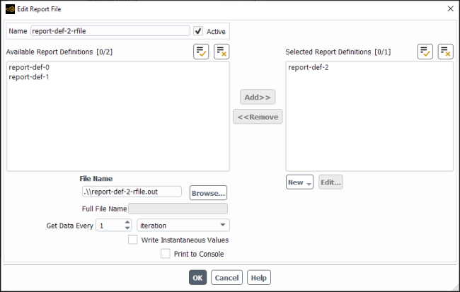
Controls
- Name
editable field displaying the name of the report file.
- Active
check box (enabled by default) that determines if the file is written during the solution calculation.
- Available Report Definitions
lists all of the existing report definitions not currently part of this report file.
- Add>>
moves the selected report definition(s) to the Selected Report Definitions list.
- <<Remove
moves the selected report definition(s) to the Available Report Definitions list.
- File Name
allows you to specify the name used when the file is saved.
- Browse...
opens the Select File dialog box, allowing you to specify the location where the report file will be saved.
- Full File Name
displays the name and location of the report file once it has been saved. You can use the keyboard arrow keys to scroll within this field (<, >).
- Get Data Every
indicates the frequency that the report definition data is written to the file. The default value of 1 allows you to write to the file at every iteration or time-step. If you select flow-time, then you must specify the frequency for writing the file in units of time. Time-step and flow-time are only a valid choices when you are calculating unsteady flow.
- Print to Console
indicates whether or not the contents of the report file are printed to the console at the frequency specified in the Get Data Every field.
- Selected Report Definitions
lists all of the existing report definitions currently included in this report file.
- New
drop-down list allowing you to create new report definitions (surface, volume, force, flux, mesh, aeromechanics, dpm, expression, and user-defined).
- Edit...
allows you to modify the highlighted report definition in the Selected Report Definition list.
![]() Solution → Reports
→ Plot...
Solution → Reports
→ Plot...
Select a report plot in the Report Plot Definition dialog box and click to open the Edit Report Plot dialog box.
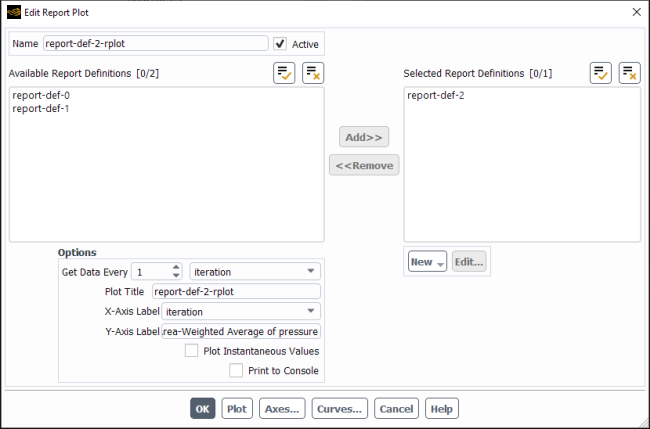
Controls
- Name
editable field displaying the name of the report plot.
- Active
check box (enabled by default) that determines if the plot is plotted during the solution calculation.
- Available Report Definitions
lists all of the existing report definitions not currently part of this report plot.
- Add>>
moves the selected report definition(s) to the Selected Report Definitions list.
- <<Remove
moves the selected report definition(s) to the Available Report Definitions list.
- Options
- Get Data Every
indicates the frequency that the report definition data is plotted. The default value of 1 allows you to write to the file at every iteration or time-step. If you select flow-time, then you must specify the frequency for plotting the data in units of time. Time-step and flow-time are only a valid choices when you are calculating unsteady flow.
- Plot Title
provide a title for the plot.
- X-Axis Label
choose whether the X-axis is flow-time or time-step.
- Y-Axis Label
enter a label for the Y-axis.
- Print to Console
indicates whether or not the contents of the report plot are printed to the console at the frequency specified in the Get Data Every field.
- Selected Report Definitions
lists all of the existing report definitions currently included in this report plot.
- New
drop-down list allowing you to create new report definitions (surface, volume, force, flux, mesh, aeromechanics, dpm, expression, and user-defined).
- Edit...
allows you to modify the highlighted report definition in the Selected Report Definition list.
- Curves...
opens the Curves Dialog Box.
- Axes...
opens the Axes Dialog Box.
The Execute on Demand dialog box allows you to run a specified user-defined function immediately. See the separate Fluent Customization Manual for details.
![]() User Defined → User Defined
→ Execute on Demand...
User Defined → User Defined
→ Execute on Demand...
Controls
- Execute on Demand
selects the user-defined function to be run.
- Execute
runs the selected function.
![]() Setup → Named
Expressions
Setup → Named
Expressions![]() New...
New...
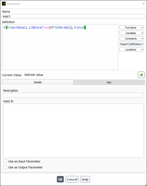
Controls
- Name
an editable field allowing you to name the expression. The Name field is not editable when the expression is in use.
- Definition
displays the formula of the expression as you create it.
- Current Value
Displays the current value of the expression.
-
Refresh Current Value

Evaluates the expression and updates the Current Value field.
- Details
This tab contains the optional description of the expression, as well as where the expression is used, and the options to set the expression as an input or output parameter.
- Description
(Optional) allows you to provide more of a description of this expression beyond the name.
- Used In
lists the locations where the expression is used.
- Use as Input Parameter
allows you to define the expression as an input parameter.
- Use as Output Parameter
allows you to define the expression as an output parameter.
- Plot
This tab allows you to plot your expression to visualize and confirm its behavior.
- Primary Independent Variable
allows you to select which variable is the independent variable.
- Count
allows you to specify the number of plot points.
- Min
sets the minimum value for the independent variable.
- Max
sets the maximum value for the independent variable.
- Secondary Independent Variable
allows you to select the secondary independent variable.
- Curves
allows you to specify the number of lines or curves to include in the plot.
- Min
sets the minimum value for the secondary independent variable.
- Max
sets the maximum value for the secondary independent variable.
- Copy to Clipboard
copies the current plot onto your clipboard.
- Reset Zoom
resets to the default zoom. You can click and drag in the plot to change the zoom level.
Drop-downs
The items in these drop-downs may be used in creating named expressions.
- Functions
lists the available functions (conditional, mathematical, and so on) that are available for constructing your expression.
- Variables
lists all of the supported variables.
- Cell Registers
lists the defined cell registers.
- Constants
lists the available pre-defined constants.
- Expressions
lists the defined expressions.
- Report Definitions
lists the defined report definitions.
- Locations
lists the available locations that you can include in your expression volume definition.
For additional information on expressions, refer to Fluent Expressions Language.
The Expression Editor dialog box is used for setting expressions
for fields, such as velocity, material density, and so on. It is opened by selecting
Expression in the drop-down list for that field, and clicking the ![]() button that appears. Refer to Directly Applied Expressions for additional information.
button that appears. Refer to Directly Applied Expressions for additional information.
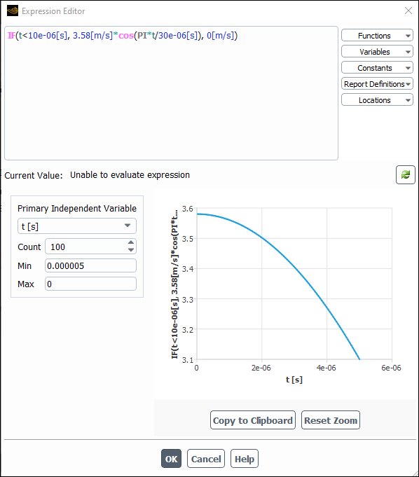
Controls
- Current Value
Displays the current value of the expression.
-
Refresh Current Value
Evaluates the expression and updates the Current Value field.
- Primary Independent Variable
allows you to select which variable is the independent variable.
- Count
allows you to specify the number of plot points.
- Min
sets the minimum value for the independent variable.
- Max
sets the maximum value for the independent variable.
- Secondary Independent Variable
allows you to select the secondary independent variable.
- Curves
allows you to specify the number of lines or curves to include in the plot.
- Min
sets the minimum value for the secondary independent variable.
- Max
sets the maximum value for the secondary independent variable.
- Copy to Clipboard
copies the current plot onto your clipboard.
- Reset Zoom
resets to the default zoom. You can click and drag in the plot to change the zoom level.
Drop-downs
The items in these drop-downs may be used in creating named expressions.
- Functions
lists the available functions (conditional, mathematical, and so on) that are available for constructing your expression.
- Variables
lists all of the supported variables.
- Cell Registers
lists the defined cell registers.
- Constants
lists the available pre-defined constants.
- Expressions
lists the defined expressions.
- Report Definitions
lists the defined report definitions.
- Locations
lists the available locations that you can include in your expression volume definition.
For additional information on expressions, refer to Fluent Expressions Language.
![]() Setup → Named
Expressions
Setup → Named
Expressions![]() Manage...
Manage...
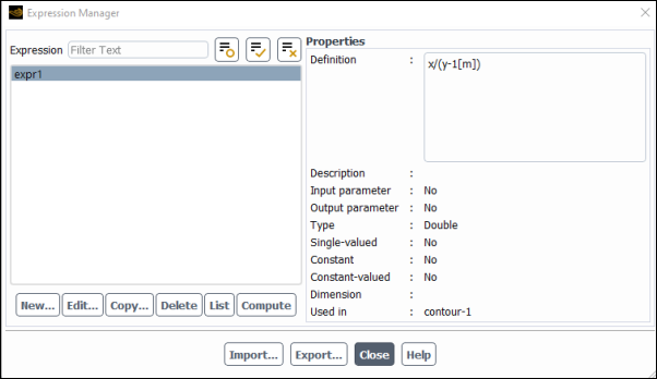
Controls
- Expression
Lists the defined named expressions.
- Properties
Lists the properties of the selected expression in the Expression list. This list is blank when no expressions are selected or when more than one expression is selected.
- New...
Opens the Expression Dialog Box, allowing you to create a new named expression.
- Edit...
(Only available when a single expression is selected) Opens the Expression Dialog Box, allowing you to edit the selected expression.
- Copy...
(Only available when a single expression is selected) Opens the Expression Dialog Box with the same definition as the selected expression. The Name field is automatically appended with a digit, but you may modify the name, if desired.
- Delete
Deletes the selected expression(s). Note that some expressions cannot be deleted if they are included in the definitions of other expressions or if they are in use elsewhere in Fluent.
- List
Prints the definition and description of all named expressions to the console.
- Compute
Computes the value of the selected expression(s) and prints the value(s) to the console.
- Import...
Opens the Select File dialog box so that you can read-in one or more expressions from a file.
- Export...
Opens the Select File dialog box so that you can export the selected expression(s) to a file.
For additional information on expressions, refer to Expression Manager.
![]() Solution → Reports
→ Definitions → New
→ Expression...
Solution → Reports
→ Definitions → New
→ Expression...
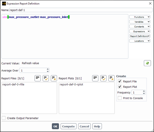
Controls
- Name
an editable field allowing you to name the expression. The Name field is not editable when the expression is in use.
- Definition
displays the formula of the expression as you create it.
- Current Value
Displays the current value of the expression.
-
Refresh Current Value
Evaluates the expression and updates the Current Value field.
- Average Over
(optional) To have Fluent calculate a running average for the Expression Report Definition you can enter a positive integer greater than 1 (the default) for Average Over.
Specifying a number greater than 1 means that Fluent will print, plot, and write the running average value of the selected variable instead of the current value of the same variable.
The value reported is averaged over the last
iterations/time steps, where is your specified Average Over value. When
the iteration/time step number is lower than , Fluent calculates the average of the available variable
values.
- Retain Instantaneous Values
appears when Average Over is set to a value greater than
1. If enabled when you are creating a new report definition, it ensures that all instantaneous values are saved in the new report file that is being created for this report definition. It also results in the Plot Instantaneous Values option being enabled in the newly created report plot.- Report Files
lists all of the report files where you can write the report definition data.
- Report Plots
lists all of the report plots where you can plot the report definition data (assuming this report has the same units as the other report definitions included in the selected report plot).
- Create
- Report File
creates a new report file that includes this report definition.
- Report Plot
creates a new report plot that includes this report definition.
- Frequency
specifies how frequently the report definition is written, plotted, or printed to the console.
- Print to Console
prints the value of the report definition to the console.
- Create Output Parameter
creates an output parameter for this report definition with the name
<report definition name>-op.- Compute
prints the value of the expression report definition to the Console.
Drop-downs
The items in these drop-downs may be used in creating expression report definitions.
- Functions
lists the available functions (conditional, mathematical, and so on) that are available for constructing your expression.
- Variables
lists all of the supported variables.
- Cell Registers
lists the defined cell registers.
- Constants
lists the available pre-defined constants.
- Expressions
lists the defined expressions.
- Report Definitions
lists the defined report definitions.
- Locations
lists the available locations that you can include in your expression report definition.
For additional information on expression report definitions, refer to Expression Report Definition.
![]() Results → Surface
→ Create → Expression
Volume...
Results → Surface
→ Create → Expression
Volume...
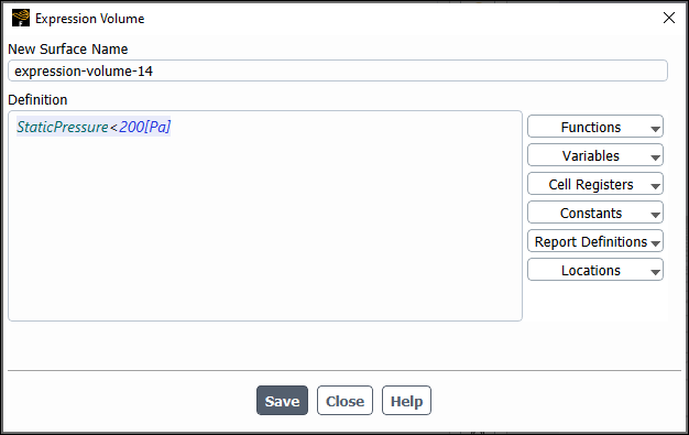
Controls
- Name
an editable field allowing you to name the expression volume.
- Definition
displays the formula of the expression volume as you create it.
- Create
creates the expression volume.
- Save
saves the changes you made to an existing expression volume.
Drop-downs
The items in these drop-downs may be used in creating expression report definitions.
- Functions
lists the available functions (conditional, mathematical, and so on) that are available for constructing your expression.
- Variables
lists all of the supported variables.
- Cell Registers
lists the defined cell registers.
- Constants
lists the available pre-defined constants.
- Expressions
lists the defined expressions.
- Report Definitions
lists the defined report definitions.
- Locations
lists the available locations that you can include in your expression volume definition.
For additional information on expression report definitions, refer to Expression Report Definition.
The Face Count Report Definition dialog box allows you to create a report definition for the reporting of a face count (that is, the number of faces within one or more boundary zones), as described in Mesh Report Definitions.
![]() Solution → Reports
→ Definitions → New
→ Mesh Report → Face Count...
Solution → Reports
→ Definitions → New
→ Mesh Report → Face Count...
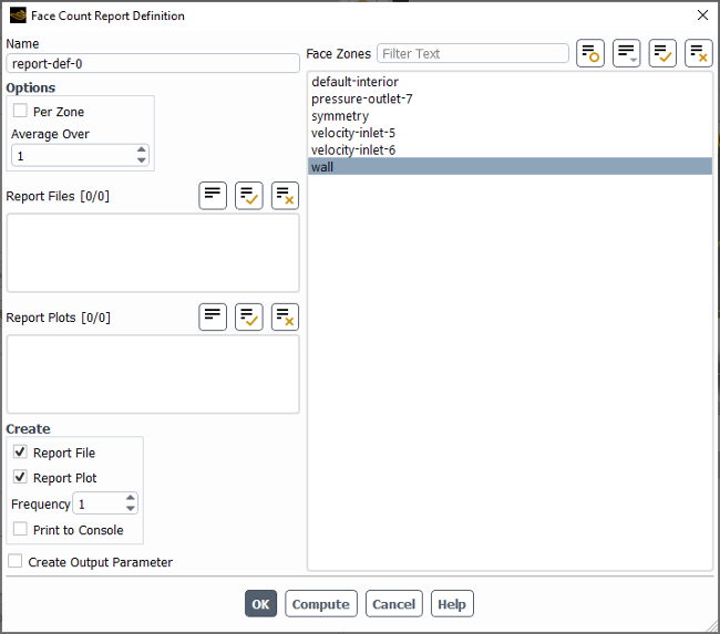
Controls
- Name
specifies the name of the report definition.
- Options
- Per Surface
enables the reporting of the face count individually for each of the selected zones (rather than reporting the sum from all of the selected zones).
- Average Over
specifies the number of iterations / time steps over which the face count is averaged when written, plotted, and/or printed. The default value of
1means that no averaging is performed (that is, only the current face count is reported), and higher values yields a running average. When the iteration / time step number is lower than the specified value, Fluent calculates the average of the available face count values.- Retain Instantaneous Values
enables the retention of instantaneous values in any report file definition or report plot definition that is associated with this report definition. This option is only available if Average Over is set to a value greater than
1.
- Report Files
allows you to select existing report file definitions to which you want to write face count data from this report definition.
- Report Plots
allows you to select existing report plot definitions to which you want to include face count data from this report definition. Note that the units used in these report plots may not be suitable for the face count data.
- Create
- Report File
creates a new report file definition for the data from this report definition.
- Report Plot
creates a new report plot definition for the data from this report definition.
- Frequency
specifies how frequently the report definition is written, plotted, and/or printed to the console.
- Print to Console
enables the printing of the face count data from this report definition to the console during the calculation.
- Create Output Parameter
creates an output parameter for this report definition with the name <report_definition_name>
-op.- Face Zones
allows you to select the face zones for which you want to report the number of faces.
- OK
creates / saves the report definition.
- Compute
computes the face count within the selected zone(s) and prints to the console.
The Field Function Definitions dialog box allows you to check, rename, save, load, and delete custom field functions that you defined in the Custom Field Function Calculator Dialog Box. See Manipulating, Saving, and Loading Custom Field Functions for details about the items below.
The Field Function Definitions dialog box is opened from the Custom Field Function Calculator Dialog Box.
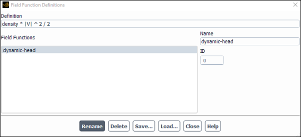
Controls
- Definition
displays the function selected in the Field Functions list. This display is for informational purposes only; you cannot edit it.
- Field Functions
contains a selectable list of custom field functions. When you select a function, its definition will appear in the Definition box and its name will appear in the Name text entry box.
- Name
displays the name of the currently selected field function. You can enter a new name in this box if you want to rename the function.
- ID
reports the ID number of the selected function. The field function at the top of the list has an ID of 0, the second function has an ID of 1, and so on.
- Rename
changes the name of the selected function to the name specified in the Name text entry box.
- Delete
deletes the selected field function.
- Save...
opens The Select File Dialog Box, where you can specify a file in which to save all of the functions in the Field Functions list.
- Load...
opens the Select File dialog box, where you can specify a file from which to read custom field functions (that is, a file that you saved using the button above).
![]() Solution → Reports
→ Definitions → New
→ Flux Report
Solution → Reports
→ Definitions → New
→ Flux Report
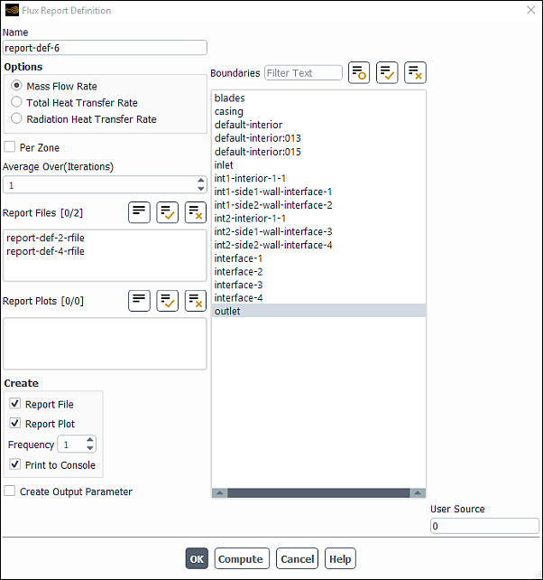
Controls
- Name
specifies the name of the report definition.
- Options
- Mass Flow Rate
specifies that the mass flow rate is computed for the selected boundary zones.
- Total Heat Transfer Rate
specifies that the total heat transfer rate is computed for the selected boundary zones.
- Total Sensible Heat Transfer Rate
specifies that the total sensible heat transfer rate is computed for the selected boundary zones. It reports the total energy flux as defined in Equation 5–5 in the Theory Guide.
- Radiation Heat Transfer Rate
specifies that the radiation heat transfer rate is computed for the selected boundary zones.
- Pressure Work Rate
specifies that the pressure work rate is computed for the selected boundary zones. This rate is the energy transfer due to pressure when a fluid zone undergoes normal zone motion relative to an adjacent solid zone (for further details, see Equation 25–1 in the Theory Guide). This pressure work is on the fluid side only, not on the solid side. This option is only available when the energy equation is enabled, the absolute velocity formulation is selected, and the Frame Motion and/or Mesh Motion option is enabled in the Fluid dialog box.
- Viscous Work Rate
specifies that the viscous work rate is computed for the selected boundary zones, which is the integral of the product of viscous stress with velocity over the external boundary of the domain with the boundary normal directed inside (for further details, see Equation 25–2 in the Theory Guide). Note that after reading case and data files into Ansys Fluent, the viscous work rate is zero. You need to run at least one iteration or time step to obtain the viscous work rate value. This item is available only when the energy equation is enabled and the pressure-based solver is selected.
- Film Mass Flow Rate
(available only when the Eulerian wall film model is enabled) specifies that the mass flow rate is computed for the selected boundary zone(s).
- Film Heat Transfer Rate
(available only when the Eulerian wall film model is enabled) specifies that the film heat transfer rate is computed for the selected boundary zone(s).
- Phase
contains a list of all of the phases in the problem that you have defined. This is available when the VOF, mixture, or Eulerian multiphase model is enabled.
- Per Zone
specifies whether or not the chosen field variable is calculated from all of the selected boundary zones combined (default) or individually on each of the selected boundary zones.
- Average Over (Time-Steps), Average Over (Iterations)
(optional) To have Fluent calculate a running average for the Flux Report Definition you can enter a positive integer greater than 1 (the default) for Average Over.
Specifying a number greater than 1 means that Fluent will print, plot, and write the running average value of the selected variable instead of the current value of the same variable.
The value reported is averaged over the last
iterations/time steps, where is your specified Average Over value. When
the iteration/time step number is lower than , Fluent calculates the average of the available variable
values.
- Retain Instantaneous Values
appears when Average Over is set to a value greater than
1. If enabled when you are creating a new report definition, it ensures that all instantaneous values are saved in the new report file that is being created for this report definition. It also results in the Plot Instantaneous Values option being enabled in the newly created report plot.- Report Files
lists all of the report files where you can write the report definition data.
- Report Plots
lists all of the report plots where you can plot the report definition data (assuming this report has the same units as the other report definitions included in the selected report plot).
- Create
- Report File
creates a new report file that includes this report definition.
- Report Plot
creates a new report plot that includes this report definition.
- Frequency
specifies how frequently the report definition is written, plotted, or printed to the console.
- Print to Console
prints the value of the report definition to the console.
- Create Output Parameter
creates an output parameter for this report definition with the name
<report definition name>-op.- Report Type
selects the integration method used on the selected cell zones. The available report types are the same as those in the Volume Integrals Dialog Box. See Volume Integration for details.
- Boundaries
contains a selectable list of valid boundary zones for flux reporting.
- OK
creates the report definition.
- Compute
computes the value of the report definition at the selected zone(s) and prints to the console.
![]() Solution → Reports
→ Definitions → New
→ Force Report → Force...
Solution → Reports
→ Definitions → New
→ Force Report → Force...
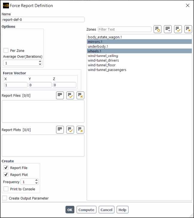
Controls
- Name
specifies the name of the report definition.
- Options
- Per Zone
specifies whether or not the force for multiple walls zones should be monitored on each wall zone separately. When this option is turned off (the default), Fluent computes and monitors the total force for all of the selected walls zones combined together.
- Average Over (Time-Steps), Average Over (Iterations)
(optional) To have Fluent calculate a running average for the Force Report Definition you can enter a positive integer greater than 1 (the default) for Average Over.
Specifying a number greater than 1 means that Fluent will print, plot, and write the running average value of the selected variable instead of the current value of the same variable.
The value reported is averaged over the last
iterations/time steps, where is your specified Average Over value.
When the iteration/time step number is lower than , Fluent calculates the average of the available variable
values.
- Retain Instantaneous Values
appears when Average Over is set to a value greater than
1. If enabled when you are creating a new report definition, it ensures that all instantaneous values are saved in the new report file that is being created for this report definition. It also results in the Plot Instantaneous Values option being enabled in the newly created report plot.
- Force Vector
contains the components of the force vector.
- X,Y,Z
are the components of the force vector along which the forces will be computed.
- Report Files
lists all of the report files where you can write the report definition data.
- Report Plots
lists all of the report plots where you can plot the report definition data (assuming this report has the same units as the other report definitions included in the selected report plot).
- Create
- Report File
creates a new report file that includes this report definition.
- Report Plot
creates a new report plot that includes this report definition.
- Frequency
specifies how frequently the report definition is written, plotted, or printed to the console.
- Print to Console
prints the value of the report definition to the console.
- Create Output Parameter
creates an output parameter for this report definition with the name
<report definition name>-op.- Zones
lists the zones you can select for force computation.
- OK
creates the report definition.
- Compute
computes the value of the report definition at the selected zone(s) and prints to the console.
The Fuse Face Zones dialog box allows you to fuse boundaries (that is, remove duplicate nodes and faces and delete artificial internal boundaries) created by assembling multiple mesh regions. (See Reading Multiple Mesh/Case/Data Files for details on importing such meshes.) See Fusing Face Zones for information about using this dialog box.
![]() Domain
→ Zones → Combine... → Fuse...
Domain
→ Zones → Combine... → Fuse...
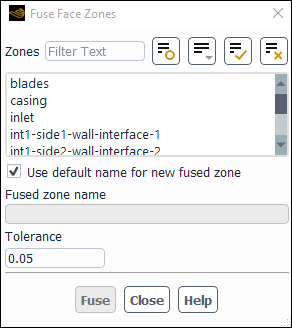
Controls
- Zones
contains a list of face zones from which you can select the boundaries to be fused.
- Use default name for new fused zone
specifies whether to use an automatically generated default name for the fused zone.
- Fused zone name
specifies the desired name for the fused zone if Use default name for new fused zone is disabled.
- Tolerance
is a fraction of the minimum edge length of the face, used to determine whether or not nodes are coincident. If all of the appropriate faces do not get fused using the default Tolerance, you should increase it and attempt to fuse the zones again. The Tolerance should not exceed 0.5, or you may fuse the wrong nodes.
- Fuse
fuses the selected zones. It is enabled only when you have selected a minimum of two zones.
The Gap Model dialog box allows you to create gap regions for use with dynamic meshes (see Using Dynamic Meshes), overset meshes (see Overset Meshes), and/or sliding meshes (see Using Sliding Meshes) to simulate flow through narrow gaps that open or close over time (such as in a valve or rotary pump). For information about using this dialog box, see Controlling Flow in Narrow Gaps for Valves and Pumps.
![]() Domain → Mesh
Models → Gap Model...
Domain → Mesh
Models → Gap Model...
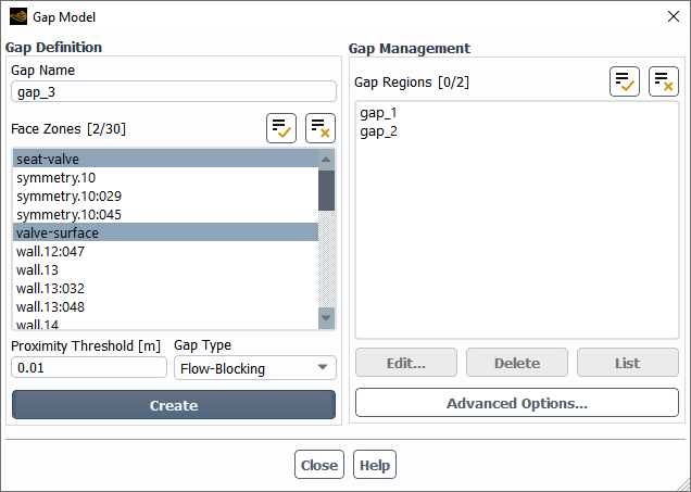
Controls
- Gap Definition
allows you to create one or more gap regions. A gap region is made up of two or more face zones, so that when one moves within a specified proximity threshold distance of another, the fluid cells within the threshold of the zones are marked, and then the flow in the cells is blocked or decelerated.
- Gap Name
specifies the name of the gap region created by the button. It cannot consist solely of numbers.
- Face Zones
allows you to select the two or more face zones that make up the gap region created by the button.
- Proximity Threshold
defines the maximum distance between the face zones when flow blockage / deceleration occurs in the gap region created by the button.
- Gap Type
defines the type of the gap region. A Flow-Blocking type completely blocks the flow in the gap region, as a numerical zero-mass-flux boundary condition is applied at the boundary faces of the marked region so that the marked cells no longer participate in the solution. A Flow-Modeling type decelerates the flow in the cells of the marked region by manipulating the viscosity or source terms.
- Gap Reynolds Number
defines the intended Reynolds number in the gap region, and thus determines the level of sealing. A lower Gap Reynolds Number results in better sealing. It can be estimated according to Equation 6–4. This drop-down list is only available when Flow-Modeling is selected for the Gap Type.
creates a gap region.
- Gap Management
allows you to manage existing gap regions and set advanced controls for the simulation.
- Gap Regions
allows you to select gap regions that you want to manage using the other buttons in the group box.
opens the Edit Gap Region Dialog Box, which you can use to edit or complete the definition of a single selected gap region.
deletes the selected gap regions.
prints information in the console about the selected gap regions.
opens the Advanced Options Dialog Box, where you can define additional options (such as the level of solution stabilization for the simulation).
The General Adaption Controls dialog box allows you to specify the general settings that Fluent uses when adapting the mesh. See Refining and Coarsening for details.
![]() Domain → Adapt
→ Controls...
Domain → Adapt
→ Controls...
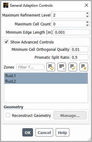
Controls
- Maximum Refinement Level
controls the number of levels of refinement used to split cells during the adaption. A value of zero places no limits on the number of levels.
- Maximum Cell Count
sets an approximate limit to the total cell count of the mesh. Fluent uses this value to determine when to stop marking cells for refinement. A value of zero places no limits on the number of cells. This field is only available with the PUMA adaption method.
- Minimum Edge Length
sets an approximate limit to the edge length for cells that are considered for refinement. Even if a cell is marked for refinement, it will not be refined if (for 3D) its volume is less than the cube of this field or (for 2D) its area is less than the square of this field. The default value of zero places no limits on the size of cells that are refined.
- Show Advanced Controls
reveals additional advanced options for adaption.
- Additional Refinement Layers
allows you to specify additional cell layers for refining the mesh. This field is only available for transient simulations.
- Prismatic Split Ratio
sets the split ratio for the cells as part of the Prismatic Adaption option in the Manual Mesh Adaption Dialog Box or Automatic Mesh Adaption Dialog Box.
- Minimum Cell Orthogonal Quality
specifies the minimum orthogonal quality that you would like Fluent to attempt to maintain in the cells that result from adaption. Note that this value is not guaranteed to be maintained, as to do so would negatively affect the solution speed. The worse quality cells will have an orthogonal quality closer to 0 and better quality cells will have an orthogonal quality closer to 1. This field is not available for 2D cases or if the hanging node adaption method is selected.
- Zones
contains a list of cell zones from which you can select the zones in which to perform adaption (or marking). By default, all cell zones are selected.
- Geometry
contains controls for geometry-based adaption when using the PUMA adaption method.
- Reconstruct Geometry
enables geometry-based adaption, using the definitions created through the Manage Geometry-Based Adaption Dialog Box to produce refined wall zones that better conform to specified auxiliary geometry definitions.
- Manage...
opens the Manage Geometry-Based Adaption Dialog Box, which you can use to specify which wall zones conform to which auxiliary geometry definitions.
For more details, see ICM Method Post-processing.
![]() Solution → Reports
→ Definitions → New
→ Aeromechanics Report
→ Generalized/Modal Force...
Solution → Reports
→ Definitions → New
→ Aeromechanics Report
→ Generalized/Modal Force...
Controls
- Name
specifies the name of the report definition.
- Options
contains options for your aerodamping report definition.
- Per Zone
If you are modeling multiple (main) blades, enables the force value to be calculated for each dynamic mesh zone (which encompasses one main blade and possibly accompanying splitter blades).
- Report Files
lists all of the report files where you can write the report definition data.
- Report Plots
lists all of the report plots where you can plot the report definition data (assuming this report has the same units as the other report definitions included in the selected report plot).
- Create
- Report File
creates a new report file that includes this report definition.
- Report Plot
creates a new report plot that includes this report definition.
- Frequency
specifies how frequently the report definition is written, plotted, or printed to the console.
- Print to Console
prints the value of the report definition to the console.
- Force Component Type
specifies the output Real or Imaginary force on the blade.
- Wall Zones
contains a selectable list of valid walls zones for force report.
- OK
creates the report definition.
- Compute
computes the value of the report definition at the selected zone(s) and prints to the console.
The Geometry Based Adaption Controls dialog box allows you to set projections. See Performing Geometry-Based Adaption with the Hanging Node Method for details about the items below.
The Geometry Based Adaption Controls dialog box is opened from the Geometry Based Adaption Dialog Box.
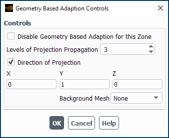
Controls
- Controls
contains parameters to define geometry based adaption.
- Disable Geometry Based Adaption for this Zone
disables the geometry reconstruction for selected zones in the domain.
- Levels of Projection Propagation
is the number of layers of the nodes you want to project.
- Direction of Projection
allows you to specify the direction in which you want to project the nodes.
- Background Mesh
allows you to load the surface mesh as a background mesh for adaption.
The Geometry Based Adaption dialog box allows you
to reconstruct the geometry while performing boundary adaption. See Geometry-Based Adaption with the Hanging Node Method for details. It is only available for 2D cases
or when the hanging node adaption method is selected (through the
mesh/adapt/set/method text command).
![]() Domain → Adapt →
More → Geometry...
Domain → Adapt →
More → Geometry...
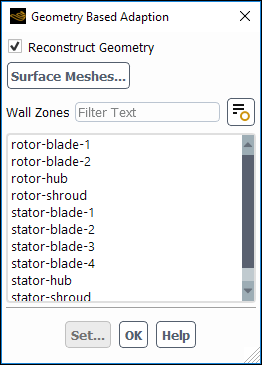
Controls
- Reconstruct Geometry
enables geometry based adaption parameters.
- Surface Meshes...
opens the Surface Meshes Dialog Box.
- Wall Zones
allows you to select the wall zones you want to adapt.
- Set...
opens the Geometry Based Adaption Controls Dialog Box.
The Import Particle Data dialog box allows you to import particle history data for display purposes in transient cases. See Importing Particle Data for details.
![]() Results → Model Specific
→ Discrete Phase → Import Particle
Data...
Results → Model Specific
→ Discrete Phase → Import Particle
Data...
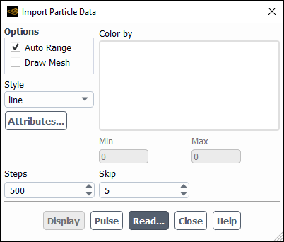
Controls
- Options
contains the check buttons that set various import particle data options.
- Auto Range
toggles between automatic and manual setting of the particle data range.
- Draw Mesh
toggles between displaying and not displaying the mesh. The Mesh Display Dialog Box is opened when Draw Mesh is selected.
- Style
allows you to select pathline style.
- Attributes...
opens the Path Style Attributes Dialog Box. This allows you to modify the line width, cylinder radius or marker size.
- Color by
contains a list from which you can select the scalar field to be used to color the particle data.
- Min,Max
allows you to set the range when Auto Range is disabled.
- Steps
sets the maximum number of steps a particle can advance.
- Skip
allows you to “thin out” the pathlines.
displays pathlines.
animates the particle positions. The Pulse button will become the Stop ! button during the animation, and you must click Stop ! to stop the pulsing.
opens a file selection dialog box where you can enter a file name and a directory for the imported data.
The Imprint Surface dialog box allows you to define a surface on top of an existing cell zone for postprocessing purposes. See Imprint Surfaces for details about the following items.
![]() Domain → Surface
→ Create → Imprint...
Domain → Surface
→ Create → Imprint...
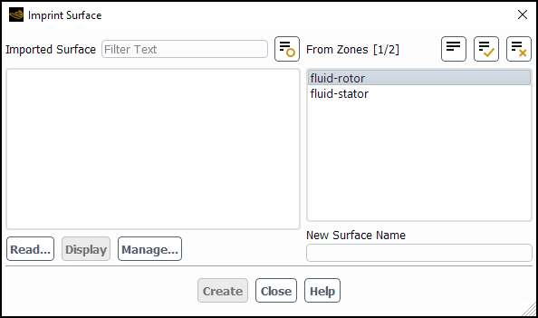
Controls
- Imported Surface
lists the surfaces that you have imported.
- Read...
opens The Select File Dialog Box, so that you can select surface files for import.
- Display
allows you to display the selected surfaces.
opens the Surfaces Dialog Box, where you can rename and delete surfaces and determine their sizes.
- New Surface Name
designates the name of the new surface. The default name format is
<original-name>(imprint)-<id>.- From Zones
allows you to select the zones where you want to import/imprint the surface mesh.
Note: If no zone is selected, then the entire domain is considered.
- Create
creates the new surface, imprinted with the mesh of the selected cell zone.
The Improve Mesh dialog box controls the quality-based smoothing of the numerical mesh. See Improving the Mesh by Smoothing and Swapping for details about the items below.
![]() Domain → Mesh
→ Improve...
Domain → Mesh
→ Improve...
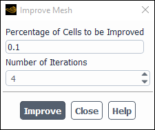
Controls
- Percentage of Cells to be Improved
sets the percentage of the total cells on which improvements are attempted. Note that the cells selected for improvement are in the areas of the mesh that exhibit the lowest orthogonal quality.
- Number of Iterations
defines the number of successive smoothing sweeps performed on the mesh.
- Improve
initiates the desired number of smoothing iterations.
The Injections dialog box allows you to create, delete, and list discrete phase injections, and access the Set Injection Properties Dialog Box and the Set Multiple Injection Properties Dialog Box, in which you can set the properties for the injections. See Creating and Modifying Injections for details.
![]() Physics → Model Specific
→ Discrete Phase
→ Injections...
Physics → Model Specific
→ Discrete Phase
→ Injections...
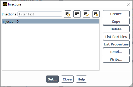
Controls
- Injections
contains a list from which you can select one or more injections in order to set, copy, or modify properties, or delete or list injections.
- Create
creates a new injection and opens the Set Injection Properties Dialog Box, in which you can set its properties.
- Copy
creates a new injection with the same properties as the selected injection and opens the Set Injection Properties Dialog Box where the new injection’s properties can be modified.
- Delete
deletes the injection(s) selected in the Injections list.
lists the initial conditions for the particle streams in the injection(s) selected in the Injections list.
lists the properties of the injection(s) selected in the Injections list.
- Read...
opens The Select File Dialog Box where you will select the injection file to read in.
- Write...
allows you to select the injection from the list and write it to a file.
- Set...
opens the Set Injection Properties Dialog Box for the injection selected in the Injections list or the Set Multiple Injection Properties Dialog Box if more than one injection is selected in the Injections list.
The Input Summary dialog box allows you to report the current settings for physical models, boundary conditions, material properties, and solution parameters. See Generating a Summary Report for details about the items below.
![]() Solution → Run Calculation
→ Input Summary...
Solution → Run Calculation
→ Input Summary...
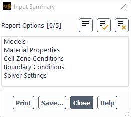
Controls
- Report Options
contains a selectable list of the information that is available for the report.
prints the selected information to the console.
opens The Select File Dialog Box, in which you can specify the filename under which to save the output of the summary report.
The Interface Creation Options dialog box allows you to define
settings that you want applied to the many-to-many mesh interfaces that are created through
the automatic method (for additional information, see Using a Non-Conformal Mesh in Ansys Fluent). It is opened by clicking the
button in the Boundary Zones group
box of the Mesh Interfaces Dialog Box. Note that this button is
only available if you have disabled the default one-to-one interface creation method by
using the define/mesh-interfaces/one-to-one-pairing? text
command.
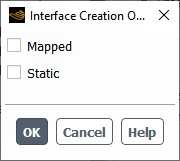
Controls
- Mapped
specifies that the mapped option is applied to all of the resulting interfaces for which at least one side of the interface consists of only solid zones. Note that the mapped option will be applied regardless of the mesh quality, and the tolerance used for mapping will be that specified in the Mapped Interface Options Dialog Box.
- Static
reduces the memory usage and processing time for interface creation (as well as for solution), especially when you are creating interfaces using many unassigned interface zones. This option will only produce correct results if the interface zones do not move or deform relative to each other at the interfaces.
The Interpreted UDFs dialog box allows you to compile user-defined functions. See the separate Fluent Customization Manual for details.
![]() User Defined → User Defined
→ Functions → Interpreted...
User Defined → User Defined
→ Functions → Interpreted...
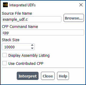
Controls
- Source File Name
sets the name of your user-defined function.
- CPP Command Name
sets the name of your C preprocessor.
- Stack Size
sets the size of the stack. Keep the default Stack Size setting of 10000, unless the number of local variables in your function will cause the stack to overflow. In this case, set the Stack Size to a number that is greater than the number of local variables used.
- Display Assembly Listing
indicates whether or not to display a listing of assembly language code in your console window as the function compiles.
- Use Contributed CPP
specifies the use of the C preprocessor that Ansys Fluent has supplied, instead of your own.
- Interpret
interprets the specified function.
The Iso-Clip dialog box allows you to interactively clip surfaces. The clipped surface consists of those points on the selected surface where the scalar field values are within the specified range. See Clipping Surfaces for details about the items below.
Controls
- Clip to Values of
contains a list from which you can select the scalar field to be used for clipping.
- Phase
allows you to select the phase when one of the multiphase models is selected in the Multiphase Model Dialog Box.
- Min, Max
set the minimum and maximum values in the clipping range. There are two ways you can set the Min and Max:
You can set a value interactively by moving the indicator in the dial above the Min or Max field with the left mouse button. This will also create a temporary surface in the graphics window. Using the dial allows you to preview the clipped surfaces before defining them. Note: Even though the clipped surface is displayed, it is only a temporary surface. To clip the surface, use the Clip button after deciding on the minimum and maximum values.
You can type in values in the Min and Max fields directly.
- Clip Surface
contains a list of surfaces from which you can select the surface to be clipped. You must select a surface to make the Clip button available.
- New Surface Name
designates the name of the surface to be created. The default is the concatenation of the surface type and an integer which is the new surface ID.
- Clip
creates the clipped surface. (The original surface will remain unchanged.)
- Compute
computes the minimum and maximum values of the scalar field across the domain, and displays them in the Min and Max boxes.
The Iso-Surface dialog box allows you to interactively create iso-surfaces. These surfaces can be iso-valued sections of an existing surface or of the entire domain. For more effective use of the slider bar, press the Compute button before using it. See Iso-surfaces for details about the items below.
Controls
- New Surface Name
designates the name of the surface to be created. The default is the concatenation of the scalar field name and an integer which is the new surface ID.
- Surface of Constant
contains a list from which you can select the scalar field which will be used for isosurfacing.
- Min
displays the minimum field value, which is computed when you click Compute.
- Max
displays the maximum field value, which is computed when you click Compute.
- Compute
computes the minimum and maximum of the scalar field across the domain and displays them in the Min and Max boxes.
- Iso-Values
sets user-specified isovalues. There are two ways you can set the Iso-Values:
You can set an isovalue interactively by moving the slider with the left mouse button. This will also create a temporary isosurface in the graphics window. Using the slider allows you to preview the isosurfaces before defining them. Note: Even though the isosurface is displayed, it is only a temporary surface. To create an isosurface, use the Create button after deciding on a particular isovalue.
You can type in isovalues in the Iso-Values field directly, separating multiple values by white space. Multiple isovalues will be contained in a single isosurface; that is, you cannot select subsurfaces within the resulting isosurface.
- From Surface
contains a list of existing surfaces from which you can select the surface to be used for isosurfacing. If you do not select a surface from the list, the isosurfacing will be performed on the entire domain.
- From Zones
contains a list of cell zones from which you can select the zone for creating an isosurface.
- Surfaces
lists the number of surfaces that will be created at once.
- Spacing
specifies the distance between surfaces.
- Create
creates the surface(s).
![]() Solution → Reports
→ Definitions → New
→ Force Report → Lift...
Solution → Reports
→ Definitions → New
→ Force Report → Lift...
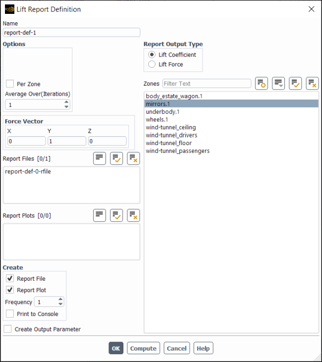
Controls
- Name
specifies the name of the report definition.
- Options
- Per Zone
specifies whether or not the lift for multiple walls zones should be monitored on each wall zone separately. When this option is turned off (the default), Fluent computes and monitors the total lift for all of the selected walls zones combined together.
- Average Over (Time-Steps), Average Over (Iterations)
(optional) To have Fluent calculate a running average for the Lift Report Definition you can enter a positive integer greater than 1 (the default) for Average Over.
Specifying a number greater than 1 means that Fluent will print, plot, and write the running average value of the selected variable instead of the current value of the same variable.
The value reported is averaged over the last
iterations/time steps, where is your specified Average Over value.
When the iteration/time step number is lower than , Fluent calculates the average of the available variable
values.
- Retain Instantaneous Values
appears when Average Over is set to a value greater than
1. If enabled when you are creating a new report definition, it ensures that all instantaneous values are saved in the new report file that is being created for this report definition. It also results in the Plot Instantaneous Values option being enabled in the newly created report plot.
- Force Vector
contains the components of the force vector.
- X,Y,Z
are the components of the force vector along which the forces will be computed.
- Report Files
lists all of the report files where you can write the report definition data.
- Report Plots
lists all of the report plots where you can plot the report definition data (assuming this report has the same units as the other report definitions included in the selected report plot).
- Create
- Report File
creates a new report file that includes this report definition.
- Report Plot
creates a new report plot that includes this report definition.
- Frequency
specifies how frequently the report definition is written, plotted, or printed to the console.
- Print to Console
prints the value of the report definition to the console.
- Create Output Parameter
creates an output parameter for this report definition with the name
<report definition name>-op.- Report Output Type
- Lift Coefficient
specifies the report definition as a unitless quantity.
- Lift Force
specifies that the report definition has units of force.
- Zones
lists the zones you can select for lift coefficient or drag lift computation.
- OK
creates the report definition.
- Compute
computes the value of the report definition at the selected zone(s) and prints to the console.
![]() Results → Graphics
→ LICs → New...
Results → Graphics
→ LICs → New...
The Line Integral Convolution dialog box allows you to create a line integral convolutions (LIC) plot. Refer to Displaying Line Integral Convolutions (LICs) for additional information.
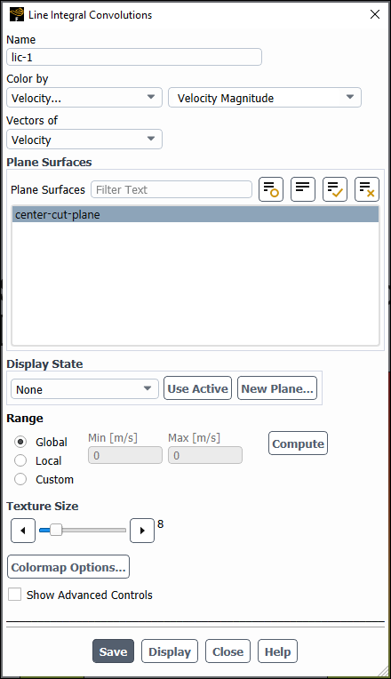
Controls
- Name
designates the name of the LICs plot.
- Color by
drop-down lists for the category and field variable used to color the plot.
- Vectors of
drop-down list specifying whether the vectors represent velocity or relative velocity.
- Phase
(Multiphase only) specifies the phase that the colors apply to.
- Vectors of
contains a list from which you can select the vector field to be plotted.
- Phase
(Multiphase only) specifies the phase for the velocity or relative velocity vectors.
- Plane Surfaces
list of planar surfaces available for displaying the LICs plot.
- Display State
specifies the display state that is associated with this graphics object.
- drop-down list of display states
selectable list of all the existing display states associated with this case.
creates a display state that matches the settings of the active graphics window and assigns it to this graphics object (this association is only saved after you click ).
- New Plane...
opens the Plane Surface Dialog Box in the Fluent User's Guide.
- Range
specifies how the range is computed.
- Global
indicates that the range is computed based on the entire domain.
- Local
indicates that the range is computed based on the selected surface(s).
- Custom
allows you to manually specify the Min and Max fields.
computes the minimum and maximum values of the field variable coloring the LICs. If Global is selected, the range is computed based on the entire domain, if Local is selected, the range is computed based on the selected surface(s).
- Texture Size
controls the size (in 100's of pixels) of the texture image used in the convolution.
- Colormap Options...
opens the Colormap Dialog Box in the Fluent User's Guide, allowing you to customize the colormap for this graphics object.
- Show Advanced Options
exposes additional advanced controls.
- Intensity Factor
scales the intensity levels of the convolution results up or down. You can use this to control the brightness or contrast of the resulting image.
- Image Filter
applies an image filter to the convolutions.
None—no filter applied.
Mild Sharpen—provides a mild increase in the focus or contrast of the texture image.
Strong Sharpen—provides a stronger increase in the focus or contrast of the texture image.
Mild Emboss—creates shadowing and highlights to give edges a raised effect on features in the image.
Strong Emboss—a stronger version of the Mild Emboss option. This will also result in the loss of color in areas with little definition before the filter was applied.
- Normalize
normalizes the vector field magnitude during the integration. The effectiveness of the convolution can be very sensitive to the vector field magnitude, so normalization is typically done to maintain a clear definition of the flow field and in particular, the location of singularities.
saves the settings of the plot as they currently appear in the dialog box.
displays a plot with the settings shown in the dialog box. Note that this button does not save the settings, so if you modify settings and display the updated plot, you must click to preserve these settings before closing the dialog box.
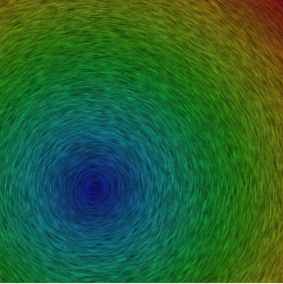
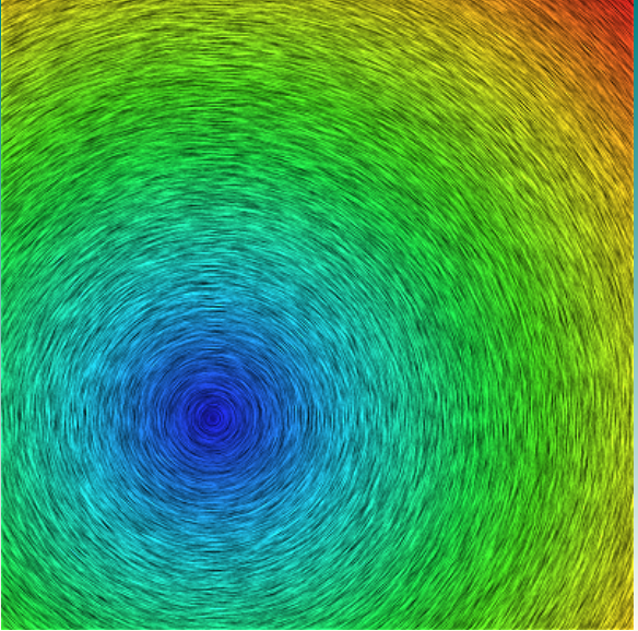

The Line/Rake Surface dialog box allows you to interactively create line and rake surfaces. A rake is a linear, uniform distribution of points between two endpoints. See Line and Rake Surfaces for details about the items below.
Controls
- Options
contains options related to the line tool. See Using the Line Tool for details about using this feature.
- Line Tool
enables the line tool.
- Reset
resets the line tool to its default position.
- Type
selects line or rake as the surface to be created.
- Number of Points
defines the number of points in the rake surface (inactive for line surfaces).
- End Points
designates the coordinates of the first point (x0, y0, z0) and the last point (x1, y1, z1).
- Select Points with Mouse
allows you to select endpoints with the mouse. You can select endpoints by clicking on locations in the active window with the mouse-probe button. (See Controlling the Mouse Button Functions for information about setting mouse button functions.)
- New Surface Name
designates the name of the new surface. The default is the concatenation of the surface type and an integer which is the new surface ID.
- Create
creates the surface.
The Manual Mesh Adaption dialog box allows you to manually adapt your mesh. See Refining and Coarsening for details.
![]() Domain → Adapt →
Manual...
Domain → Adapt →
Manual...
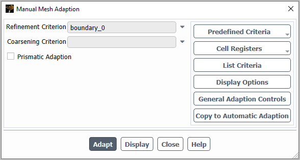
Controls
- Refinement Criterion
specifies the cell register or expression that Fluent will use during the calculation to determine which cells to refine.
- Coarsening Criterion
specifies the cell register or expression that Fluent will use during the calculation to determine which cells to coarsen.
- Prismatic Adaption
specifies that prismatic cells are adapted anisotropically. This option is only available with the PUMA adaption method.
allows you to select from a list of commonly used criteria for adapting the mesh (for a description of the list, see Predefined Criteria for Adaption); if one is selected, Fluent will automatically generate the necessary cell registers and/or expressions for refinement and coarsening, and define the settings in the Manual Mesh Adaption dialog box and General Adaption Controls Dialog Box accordingly. Depending on your selection, you may be prompted to complete the setup by defining fields in the Adaption Criteria Settings Dialog Box.
allows you to create new cell registers and manage existing ones, which may then be selected from the Refinement Criterion and/or Coarsening Criterion drop-down lists.
prints to the console the number of cells marked for refinement, the number of cells marked for coarsening, and the number marked for both operations.
opens the Display Options - Adaption Dialog Box.
opens the General Adaption Controls Dialog Box, where you can specify the general settings that Fluent uses when adapting the mesh.
copies the settings to the Automatic Mesh Adaption Dialog Box, where you can create adaption criteria which can be applied during the solution.
performs adaption based on the settings in this dialog box.
The Manage Adaption Criteria dialog box allows you to manage criteria for automatic mesh adaption. See Refining and Coarsening for details.
![]() Domain → Adapt
→ Manage...
Domain → Adapt
→ Manage...
Controls
- Adaption Criteria
lists the defined criteria for automatic adaption during a calculation.
- Properties
displays information about the criterion selected in the Adaption Criteria list.
- New...
opens the Automatic Mesh Adaption Dialog Box, where you can create new automatic adaption criteria.
- Edit...
opens the Automatic Mesh Adaption Dialog Box, where you can edit the criterion selected in the Adaption Criteria list.
- Deactivate
deactivates the criterion selected in the Adaption Criteria list, so that it is not applied during the calculation.
- Activate
activates the criterion selected in the Adaption Criteria list, so that it is applied during the calculation.
- Delete
deletes the criterion selected in the Adaption Criteria list.
The Manage Geometry-Based Adaption dialog box allows you to manage definitions for geometry-based adaption with the PUMA adaption method. It is opened by clicking the button under the Show Advanced Controls option in the General Adaption Controls Dialog Box. See Refining and Coarsening for details.
Controls
- Wall Zone
allows you to select the wall zone to which you want geometry-based adaption applied.
- Auxiliary Geometry Definition
allows you to select the auxiliary geometry definition to which you want the selected Wall Zone to conform. For details on creating auxiliary geometry definitions, see Managing Auxiliary Geometry Definitions.
- Geometry-Based Adaption Zones
lists the pairings of wall zones and auxiliary geometry definitions that you have created through the button. You can make a single selection from this list and click the button if you want delete the pairing.
creates a pairing (listed under Geometry-Based Adaption Zones) of the selected Wall Zone and Auxiliary Geometry Definition.
allows you to revise which Auxiliary Geometry Definition is paired with a given Wall Zone.
deletes the selected pairing under Geometry-Based Adaption Zones.
deletes all of the pairings under Geometry-Based Adaption Zones.
The Manage Sponge Layers dialog box allows you to define sponge layers at boundary zones (so that the density is blended from the value calculated by the solver to user-specified far-field values), in order to eliminate non-physical pressure wave reflections from boundary zones in transient simulations of compressible flows with the pressure-based solver. For further details, see Sponge Layers.
Controls
- Sponge Layers
lists the existing sponge layer definitions.
- Properties
lists the properties of the selected sponge layer in the Sponge Layers list. This list is blank when a sponge layer is not selected.
- New...
opens the Sponge Layer Dialog Box, allowing you to create a new sponge layer definition, which by default is active.
- Edit...
opens the Sponge Layer Dialog Box, allowing you to edit the definition selected in the Sponge Layers list.
- Activate
activates the selection in the Sponge Layers list, so that it is used when the calculation is run.
- Deactivate
deactivates the selection in the Sponge Layers list, so that it is not used when the calculation is run.
- Delete
deletes the definition that is selected in the Sponge Layers list.
The Mapped Interface Options dialog box allows you to update which mesh interfaces use the mapped option and the related settings (see The Mapped Option for additional information). It is opened by selecting a many-to-many mesh interface and clicking the button in the Mesh Interfaces group box of the Mesh Interfaces Dialog Box.
Controls
- Mapped Interface
contains options related to mapped interface specification.
- Auto (Tolerance-Based)
specifies that all mesh interfaces that have interface zones that penetrate each other are automatically defined as Mapped interfaces (provided that at least one side of each interface consists only of solid zones).
- Tolerance
- Local Edge Length Factor
(when enabled) allows you to specify the multiplier that Fluent uses with the smallest edge length of the interface zones to calculate the tolerance for mapping. Disabling Local Edge Length Factor allows you to specify an absolute value for the tolerance. Note that this does not overwrite any locally specified tolerance in the Edit Mesh Interfaces dialog box.
- Solution Controls
- Mapping Frequency
specifies how often calculation values are interpolated across mapped interfaces.
- Under-Relaxation Factor
allows you to reduce the rate of change per iteration of physical quantities across mapped interfaces to aid with convergence. For additional information on setting under-relaxation factors, see Setting Under-Relaxation Factors.
- Update
applies the selection(s) made in the Mapped Interface Options dialog box. This button is grayed out until you make enable / disable the Auto (Tolerance-Based) option; it also returns to being grayed out once it is clicked.
Note: Enabling the Auto (Tolerance-Based) option and clicking applies these selections globally for all relevant interfaces. Once you click you can return to the Mesh Interfaces dialog box to modify local settings for individual interfaces.
The Material Editor dialog box allows you create new materials for realistic rendering. Refer to Creating Custom Realistic Materials for additional information on using the Material Editor dialog box.
![]() View → Graphics
→ Material Editor...
View → Graphics
→ Material Editor...
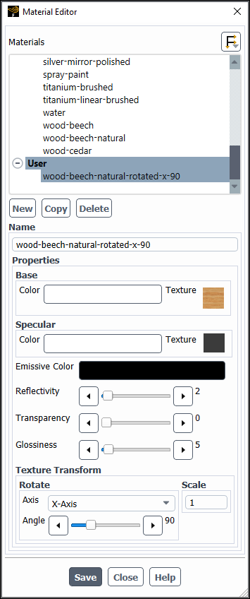
Controls
- Materials
lists the available realistic materials.
creates a new material with default properties.
creates a new material with the properties of the selected Material.
removes the material from the Materials list and from any mesh objects referencing that material. You can only delete user-defined materials; the default materials cannot be deleted.
- Properties
lists the editable properties that define the material's appearance.
- Base Color
specifies the bulk color of the material. Texture is a non-editable field that indicates the base texture associated with the material, if there is one. You can hover over the texture image to see an enlarged picture of the texture.
- Specular Color
specifies the highlight color seen due to lighting effects. Texture is a non-editable field that indicates the specular texture associated with the material, if there is one. You can hover over the texture image to see an enlarged picture of the texture.
- Emissive Color
specifies the color emitted from the material.
- Reflectivity
specifies how reflective the material appears.
- Transparency
specifies how transparent the material appears.
- Glossiness
specifies how glossy the material appears.
- Texture Transform
provides options for modifying the appearance of the material texture.
- Rotate
controls the orientation of the texture.
- Axis
specifies the axis the texture will be rotated about.
- Angle
controls the angle (in degrees) that the texture is rotated about the selected axis.
- Scale
controls the scaling of the texture. A larger value increases the texture scaling, similarly to zooming in on the texture. Valid inputs are in the range 0.0004 to 4.
saves the current settings of any custom material.
The Measure dialog box allows you measure objects displayed in the graphics window. You can measure the distance between 2 points or the angle formed by 3 points. See Merging Zones for details.
![]() View → Graphics
→ Measure...
View → Graphics
→ Measure...
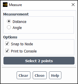
Controls
- Measurement
lists the two types of measurements that you can make:
indicates that you will be measuring the distance between two points in the graphics window when you click . You can use the left-mouse-button (LMB) or right-mouse-button (RMB) to select the points.
indicates that you will be measuring the angle between three points in the graphics window when you click . You can use the left-mouse-button (LMB) or right-mouse-button (RMB) to select the points.
- Options
contains controls for whether the points clicked in the interface automatically snap to the node, and whether the measurement details are printed to the console.
- Snap to Node
indicates that measurement clicks in the graphics window are snapped to the nearest node, when enabled. When disabled, the measurements are taken at the location where the mouse is clicked.
- Print to Console
indicates that the measurement details are printed to the console, when enabled.
- |
activates the measurement tool so that you can select the points for measuring distance () or angle ().
The Merge Zones dialog box allows you to merge multiple zones of the same type into a single zone. See Merging Zones for details.
![]() Domain → Zones
→ Combine → Merge...
Domain → Zones
→ Combine → Merge...
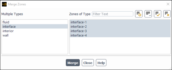
Controls
- Multiple Types
contains a selectable list of the zone types for which you can merge multiple zones. You select a type and the corresponding zones of that type will be displayed in the Zones of Type list.
- Zones of Type
contains a list from which you can select two or more zones to be merged into a single zone. The zones are of the type selected in the Multiple Types list.
- Merge
merges the selected zones into a single zone. If your case file has dynamic zones or mesh interfaces, the Warning Dialog Box will open and require your input prior to the merge.
The Mesh Interfaces dialog box allows you to automatically or manually create mesh interfaces for use with sliding meshes (see Using Sliding Meshes) or multiple reference frames (see Mesh Setup for a Multiple Moving Reference Frame), or for meshes with non-conformal boundaries (see Non-Conformal Meshes). For information about using this dialog box, see Using a Non-Conformal Mesh in Ansys Fluent.
![]() Domain → Interfaces → Mesh...
Domain → Interfaces → Mesh...
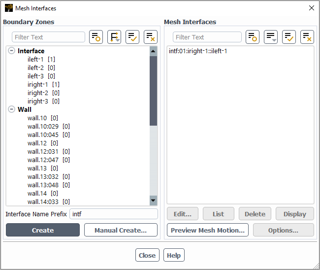
Controls
- Boundary Zones
allows you to create new mesh interfaces using the automatic or manual method. Note that the selection list at the top of the group box (which lists the boundary zones available for selection, along with a number that indicates the number of mesh interfaces that zone is a part of) is only used as part of the automatic method; when a selection is made, the Mesh Interfaces of which it is a part are also highlighted.
- Interface Name Prefix
specifies the prefix used in the names of all the mesh interfaces created automatically through the button.
opens the Interface Creation Options Dialog Box, so you can define settings that you want applied to the mesh interfaces that are created automatically through the button. This button is only available if you have disabled the default one-to-one interface creation method by using the
define/mesh-interfaces/one-to-one-pairing?text command.creates mesh interfaces using the automatic method, so that Fluent is responsible for determining which of the selected Boundary Zones can be grouped together to form the two sides of one or more mesh interfaces. Note that mesh interfaces that use the periodic or periodic repeats option cannot be created using this button, but must instead be created by disabling the one-to-one interface creation method and using the button.
opens additional dialog boxes that allow you to manually create mesh interfaces with methods or options that are not available in the Mesh Interfaces dialog box. When the default one-to-one interface creation method is enabled, this button opens the Create Mesh Interfaces, so that you can easily create many mesh interfaces between boundary zones that do not currently overlap (for example, for a sliding mesh simulation). When the one-to-one interface creation method is disabled (through the
define/mesh-interfaces/one-to-one-pairing?text command), this button opens the Create/Edit Mesh Interfaces Dialog Box, so you can create mesh interfaces that use the periodic or periodic repeats option.opens the Create/Edit Turbo Interfaces Dialog Box, so you can create turbo interfaces. This button is only available if you have disabled the default one-to-one interface creation method by using the
define/mesh-interfaces/one-to-one-pairing?text command or, before creating any one-to-one mesh interfaces, by enabling the Enable option in the Turbo Model group of the Domain ribbon tab.
- Mesh Interfaces
allows you to manage existing mesh interfaces. Note that many of the buttons in this group box are not accessible unless you make a selection from the list at the top. This list enumerates the mesh interfaces that have been created; when a selection is made, the Boundary Zones that comprise it are also highlighted.
opens the Edit Mesh Interface dialog box or (for a many-to-many mesh interface) the Edit Mesh Interfaces Dialog Box, so you can edit the name or (for a many-to-many mesh interface) the name, list of interface zones assigned to the interface, and/or interface options.
prints information about the selected mesh interface(s) in the console.
deletes the selected mesh interfaces.
allows you to display the selected mesh interface in the graphics window. Note that after you have selected a mesh interface, you can modify what zones are displayed by selecting / deselecting zones in the Boundary Zones list.
opens the Mesh Motion Dialog Box.
opens the Mapped Interface Options Dialog Box, where you can update which mesh interfaces use the mapped option and set global parameters for the mapped mesh interfaces. This button is only available if you selected a many-to-many mesh interface from the selection list in the Mesh Interfaces group box.
The Mesh Morpher/Optimizer dialog box allows you to use the mesh morpher/optimizer to deform the mesh in order to solve shape optimization problems. You can deform the mesh manually, allow a built-in optimizer to define the deformation in order to minimize an objective function, or use Design Exploration in Ansys Workbench to easily explore a variety of deformation scenarios. See Using the Mesh Morpher/Optimizer for further details.
![]() Design → Parameter-Based → Optimizer...
Design → Parameter-Based → Optimizer...
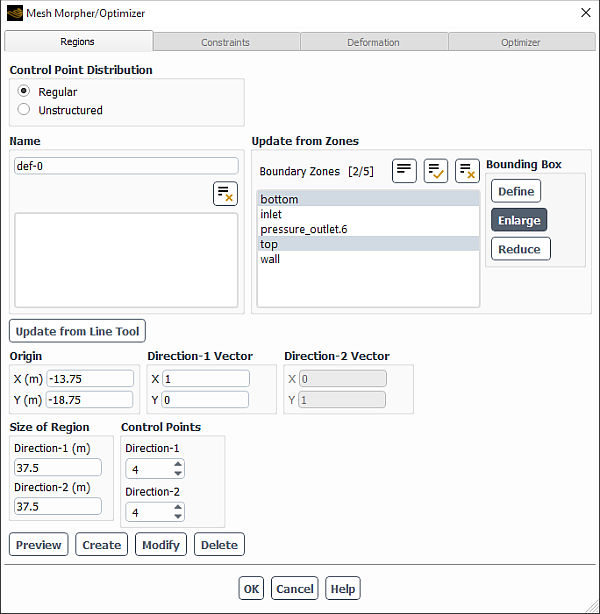
Controls
- Regions
tab allows you to define the regions of the domain where the mesh will be deformed in order to optimize the shape.
- Control Point Distribution
allows you to select the way in which you will define the locations of the control points, as well as the kinds of motions you can apply.
- Regular
specifies that the control points will be spread in a regular distribution throughout the entire deformation region. The number of control points along each of the defining direction vectors will be specified in the Control Points group box. The motion of the control points will be limited to translations, as the ability to define rotational or radial motions will not be available.
- Unstructured
specifies that control point locations will be specified by right-clicking with the mouse on boundary zones, distributing an approximate number throughout a zone, or by entering coordinates, using the Define Control Points Dialog Box. The motion of the control points will be able to be defined as translations, as rotations about a point / axis, or radially about a point / axis.
- Name
provides controls for the deformation regions you are defining. The upper text-entry box defines the name of the region that is created when you click the button. The lower selection list allows you to select a region that has already been created, in order to display it in the graphics window, modify the settings via the button, or delete the region via the button.
- Update from Zones
allows you to create a bounding box that defines the deformation region.
- Boundary Zones
specifies the boundary zones that will be used to generate a bounding box for the deformation region when you click the button.
- Define
updates the values in the Origin, Direction-1 Vector, Direction-2 Vector, and Size of Region group boxes based on a bounding box that encompasses the selections in the Boundary Zones list, and previews the bounding box in green in the graphics window.
- Enlarge
increases the size of the bounding box created by the button, and previews the revised bounding box in green in the graphics window.
- Reduce
decreases the size of the bounding box created by the button, and previews the revised bounding box in green in the graphics window.
updates the values in the Direction-1 Vector and Direction-2 Vector group boxes based on the settings in the plane tool. See Using the Plane Tool for information about the plane tool. This button is only available for 3D cases.
Open the Plane Surface Dialog Box to make the plane tool appear.
updates the values in the Direction-1 Vector and Direction-2 Vector group boxes based on the settings in the line tool. See Using the Line Tool for information about the line tool. This button is only available for 2D cases.
Open the Line/Rake Surface Dialog Box to make the line tool appear.
- Origin
allows you to define the Cartesian coordinates of the origin of the deformation region.
- X
defines the x coordinate of the origin of the deformation region.
- Y
defines the y coordinate of the origin of the deformation region.
- Z
defines the z coordinate of the origin of the deformation region. This number-entry box is only available for 3D cases.
- Direction-1 Vector
allows you to define a vector that acts as the first direction of the deformation region relative to the Origin.
- X
defines the x component of the first direction vector of the deformation region.
- Y
defines the y component of the first direction vector of the deformation region.
- Z
defines the z component of the first direction vector of the deformation region. This number-entry box is only available for 3D cases.
- Direction-2 Vector
defines a vector that is used to calculate the second direction of the deformation region relative to the Origin. For 2D cases, the values in the Direction-2 Vector group box are automatically defined by Ansys Fluent to be perpendicular to the Direction-1 Vector. For 3D cases, the vector defined by the Direction-2 Vector group box is projected onto a plane that intersects the Origin and is perpendicular to the vector defined in the Direction-1 Vector group box, in order to calculate the second direction.
- X
defines the x component of the vector used to calculate the second direction of the deformation region. This number-entry box is only editable for 3D cases.
- Y
defines the y component of the vector used to calculate the second direction of the deformation region. This number-entry box is only editable for 3D cases.
- Z
defines the z component of the vector used to calculate the second direction of the deformation region. This number-entry box is only available for 3D cases.
- Size of Region
allows you to define the overall dimensions of the deformation region.
- Direction-1
defines the length of the deformation region along the direction specified by the Direction-1 Vector group box.
- Direction-2
defines the length of the deformation region along the direction specified by the Direction-2 Vector group box.
- Direction-3
defines the length of the deformation region along the third axis (that is, the cross product of the vectors defined by the Direction-1 Vector and Direction-2 Vector group boxes). This number-entry box is only available for 3D cases.
- Boundary Continuity
allows you to specify whether the mesh transitions are smooth or abrupt wherever the mesh intersects with the limits of the deformation region. This group box is only available when Unstructured is selected from the Control Point Distribution list.
- Smooth Transitions
enables smooth mesh transitions wherever the mesh intersects with the limits of the deformation region, based on the creation of stationary control points at those intersections.
- Display Control Points
displays the stationary control points created when the Smooth Transitions option is enabled.
- Control Points
allows you to define the control points for the deformation regions.
- Direction-1
defines the number of control points for the deformation region selected in the Name group box along the direction specified by the Direction-1 Vector group box. This number-entry box is only available when Regular is selected from the Control Point Distribution list.
- Direction-2
defines the number of control points for the deformation region selected in the Name group box along the direction specified by the Direction-2 Vector group box. This number-entry box is only available when Regular is selected from the Control Point Distribution list.
- Direction-3
defines the number of control points for the deformation region selected in the Name group box along the third axis (that is, the cross product of the vectors defined by the Direction-1 Vector and Direction-2 Vector group boxes). This number-entry box is only available for 3D cases when Regular is selected from the Control Point Distribution list.
- Define...
opens the Define Control Points Dialog Box, which you can use to define the control points. This button is only available when Unstructured is selected from the Control Point Distribution list.
- Preview
displays (in green) the bounding box that results from the current settings in the Origin, Direction-1 Vector, Direction-2 Vector, and Size of Region group boxes.
- Create
creates a new deformation region with the name specified in the upper text-entry box of the Name group box and with the settings defined using the Origin, Direction-1 Vector, Direction-2 Vector, Size of Region, and (for regular control point distributions) Control Points group boxes. The newly created deformation region will be added to and selected in the lower Name selection list, and will be displayed (in blue) in the graphics window.
- Modify
modifies the saved settings for the deformation region selected in the lower Name selection list and displays the modified region in the graphics window.
- Delete
deletes the deformation region selected in the lower Name selection list.
- Constraints
tab allows you to define the constraints on the boundary zones, in order to limit the freedom of particular zones that fall within the deformation region(s) during the morphing of the mesh.
- Zones
allows you to select the boundary zones for which you are defining a constraint.
- Option
specifies the constraint on the boundary zones selected from the Zones list.
- Unconstrained
specifies that the boundary zones are completely free to be deformed according to the assigned parameters.
- Passive
specifies that the nodes of the boundary zones are partially constrained to varying degrees, based on their proximity to adjacent boundary zones that are fixed. The nodes in a passive boundary zone behave in a similar manner to the interior mesh nodes, in order to ensure that there is a smooth transition between fixed and unconstrained boundary zones.
- Fixed
specifies that the boundary zones are fixed and will not be deformed.
- Display
displays the selected Zones in the graphics window.
- Summary
prints a list in the console that summarizes the constraint definitions for all of the boundary zones.
- Deformation
tab allows you to define the deformation.
- Number of Parameters
defines the number of parameters available to define the motion of the control points.
- Parameter Values
allows you to define either the magnitude of deformation associated with each parameter (when you are manually specifying the deformation or using Design Exploration in Ansys Workbench to explore multiple deformation scenarios) or the bounds for each parameter (when you are using a built-in optimizer).
- par1, par2...
specify the magnitude of deformation associated with each parameter. You can enter a numeric value in the field or use the
 icon to create or assign an input parameter (see Select Input Parameter Dialog Box for details). These fields
and icons are only available when none or workbench is selected from the Optimizer drop-down list in the Optimizer tab. Note that
the value entered here will specify a length in meters for translations
and radial motions, and will specify an angle in degrees for rotations;
these units will be used regardless of what units you are using in
the case.
icon to create or assign an input parameter (see Select Input Parameter Dialog Box for details). These fields
and icons are only available when none or workbench is selected from the Optimizer drop-down list in the Optimizer tab. Note that
the value entered here will specify a length in meters for translations
and radial motions, and will specify an angle in degrees for rotations;
these units will be used regardless of what units you are using in
the case. - Apply
saves definitions for the parameter fields in the Parameter Values group box. This button is only available when none or workbench is selected from the Optimizer drop-down list in the Optimizer tab.
- Set Bounds...
opens the Parameter Bounds Dialog Box, where you can define strict minimum and maximum values for the parameters. Note that this button is not available when workbench is selected from the Optimizer drop-down list in the Optimizer tab.
opens the Motion Settings Dialog Box, where you can define the motion of the control points.
applies the current settings in the Parameter Values group box, modifies the mesh, and updates the mesh display in the graphics window. This button is only available when none is selected from the Optimizer drop-down list in the Optimizer tab.
displays a mesh check report in the console for the mesh displayed in the graphics window. This button is only available when none is selected from the Optimizer drop-down list in the Optimizer tab. The mesh check report provides volume statistics, mesh topology and periodic boundary information, verification of simplex counters, and verification of node position with reference to the
 axis for axisymmetric cases, in the same manner
as the button in the General task page (see Checking the Mesh for details).
axis for axisymmetric cases, in the same manner
as the button in the General task page (see Checking the Mesh for details).- Reset
undoes any modifications made to the mesh as a result of the button and updates the mesh display in the graphics window.
- Optimizer
tab allows you to define the settings for the optimizer.
- Optimizer
specifies which optimizer is used. The choices include none (for manual deformation); compass, newuoa, powell, rosenbrock, simplex, and torczon (for optimization in Ansys Fluent); and workbench (for optimizing using Design Exploration in Ansys Workbench). Note that workbench is only available if you have launched your Ansys Fluent session from Ansys Workbench. For information about how the built-in optimizers function or how to use Design Exploration, see Design Analysis and Optimization in the User's Guide or Working With Input and Output Parameters in Workbench in the Ansys Fluent in Workbench User's Guide, respectively.
opens the Objective Function Definition Dialog Box, where you can specify the format of the objective function that will be minimized during the optimization process. This button is not available if none or workbench is selected from the Optimizer drop-down list.
- Optimizer Settings
allows you to specify the optimizer settings. This group box is not available if none or workbench is selected from the Optimizer drop-down list.
- Maximum Number of Designs
defines the maximum number of design stages the optimizer will undergo to reach the specified objective function.
- Maximum Iterations per Design
defines the maximum number of iterations Ansys Fluent will perform for each design change.
- Optimizer Convergence Criteria
defines the convergence criteria for the optimizer.
- Initial Parameter Variation
defines how much the parameters will be allowed to vary during the initial calculations when newuoa is selected from the Optimizer drop-down list.
- Mesh Quality
allows you to enable and define a mesh quality check: if the orthogonal quality (as defined in Mesh Quality) for any cell of a mesh is less than a specified value, no solution is calculated for the mesh and Fluent proceeds to the next design stage. This group box is not available if none is selected from the Optimizer drop-down list.
- Reject Poor Quality Meshes
enables the consideration of orthogonal quality when determining whether a solution should be calculated for a mesh.
- Minimum Orthogonal Quality
defines the minimum orthogonal quality value every cell must have in order for a solution to be calculated for a mesh. Values may range from
0–1(where0represents the worst quality).
- Case and Data File Sets
allows you to enable the automatic saving of intermediate case and data files at specified intervals during the optimization run, so that you can restart an interrupted solution in the same or a different Fluent session without increasing the overall number of design iterations needed to reach convergence. This group box is not available if none or workbench is selected from the Optimizer drop-down list.
- Save Every
specifies the frequency (in number of design iterations) that you want intermediate case and data file sets saved. Note that the default value is 0, which specifies that no intermediate files will be saved.
- Maximum Number Retained
specifies the maximum number of intermediate case and data files sets you want to retain. After the maximum limit of file sets has been saved, Ansys Fluent begins overwriting the earliest existing intermediate file set.
- File Name
specifies a root name for the intermediate case and data file sets, which will be appended with a number that represents the design iteration during which it was saved. Note that you can include a folder path in the file name if you want the files saved outside of the working folder.
- Initialization
provides settings that determine how the solution variables are treated after the mesh is deformed during the optimization process. This group box is not available if none or workbench is selected from the Optimizer drop-down list.
- Method
allows you to select one of the following:
- Initialize Data After Morphing
specifies that the solution variables should be initialized to the values defined in the Solution Initialization task page after deformation.
- Continue with Current Data
specifies that the solution variables should remain the values obtained in the previous design iteration.
- Read Data File After Morphing
specifies that the solution variables are set to the values obtained from the data file specified in the Data File Name text-entry box after deformation. This selection is not available when newuoa is selected from the Optimizer drop-down list.
- Data File Name
specifies the data file from which the solution variables are obtained when Read Data File After Morphing is selected.
- Execute Commands
allows you to specify commands (text commands or command macros) that will be run during the optimization runs of the mesh morpher/optimizer. This group box is not available if none, newuoa, or workbench is selected from the Optimizer drop-down list.
- Initial Commands
specifies the commands that will be run after the design has been modified, but before Ansys Fluent has started to run the calculation for that design stage.
- End Commands
specifies the commands that will be run after the solution has run and converged for a design stage.
opens the Optimization History Monitor Dialog Box, which allows you to plot and/or record how the value of the objective function varies with each design stage. This button is not available if none, newuoa, or workbench is selected from the Optimizer drop-down list.
- Apply
saves the settings in the Optimizer tab.
- Summary
displays a summary of the mesh morpher/optimizer settings in the console.
initiates the optimization process using the settings saved in all of the tabs of the Mesh Morpher/Optimizer dialog box. This button is not available if none or workbench is selected from the Optimizer drop-down list.
The Mixing Planes dialog box allows you to define the mixing planes for a mixing plane model. See Setting Up the Legacy Mixing Plane Model for details about using the items below.
![]() Domain → Mesh Models
→ Mixing Planes...
Domain → Mesh Models
→ Mixing Planes...
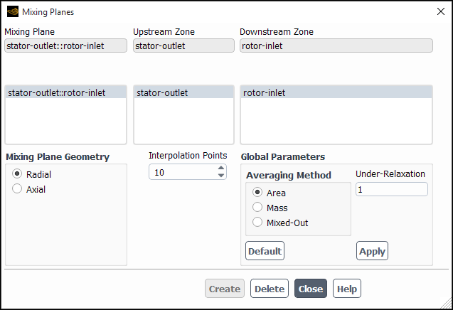
Controls
- Mixing Plane
contains a list from which you can select an existing mixing plane, and an informational field in which Ansys Fluent displays the name of the currently selected (or most recently created) mixing plane.
- Upstream Zone, Downstream Zone
contain lists from which you can select the boundaries on the upstream and downstream sides of the mixing plane, and informational fields that show the names of the zone you selected in each list. (You cannot edit these fields; the name in each field will be the name of the zone you selected in the list below it.)
- Interpolation Points
specifies the number of radial or axial locations used in constructing the boundary profiles for circumferential averaging. This item appears only in 3D.
- Mixing Plane Geometry
defines the geometry of the mixing plane interface. This item appears only in 3D.
- Radial
specifies that information at the mixing plane interface is to be circumferentially averaged into profiles that vary in the radial direction, for example,
 ,
,  .
.- Axial
specifies that circumferentially averaged profiles are to be constructed that vary in the axial direction, for example,
 ,
,  .
.
- Global Parameters
contains parameters related to the mixing plane calculation.
- Averaging Method
consists of three profile averaging methods.
- Area
is the default method and is expressed using Equation 2–17 in the Theory Guide.
- Mass
provides better representation of the total quantities than the area averaging method. It is defined by Equation 2–18 of the Theory Guide.
- Mixed-Out
is most representative of non-uniform flow profiles and is expressed using Equation 2–20 in the Theory Guide.
- Under-Relaxation
specifies the under-relaxation factor for updating the boundary values at mixing planes.
sets the specified Under-Relaxation.
sets the Under-Relaxation to its default value, as assigned by Ansys Fluent. After execution, the button becomes the Reset button.
resets the Under-Relaxation to its most recently saved value (that is, the value before was selected). After execution, the button becomes the button.
- Create
creates the specified mixing plane (and assigns it a name in the Mixing Plane field).
- Delete
deletes the mixing plane selected under Mixing Plane.
![]() Solution → Reports
→ Definitions → New
→ Force Report → Moment...
Solution → Reports
→ Definitions → New
→ Force Report → Moment...
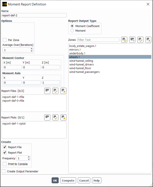
Controls
- Name
specifies the name of the report definition.
- Options
- Per Zone
specifies whether or not moments for multiple walls should be monitored on each wall separately. When this option is turned off (the default), Fluent computes and monitors the total force for all of the selected walls combined together.
- Average Over (Time-Steps), Average Over (Iterations)
(optional) To have Fluent calculate a running average for the Moment Report Definition you can enter a positive integer greater than 1 (the default) for Average Over.
Specifying a number greater than 1 means that Fluent will print, plot, and write the running average value of the selected variable instead of the current value of the same variable.
The value reported is averaged over the last
iterations/time steps, where is your specified Average Over value.
When the iteration/time step number is lower than , Fluent calculates the average of the available variable
values.
- Retain Instantaneous Values
appears when Average Over is set to a value greater than
1. If enabled when you are creating a new report definition, it ensures that all instantaneous values are saved in the new report file that is being created for this report definition. It also results in the Plot Instantaneous Values option being enabled in the newly created report plot.
- Moment Center
contains the Cartesian coordinates of the moment center.
- Moment Axis
contains the Cartesian coordinates of the moment vector to be monitored.
- Report Files
lists all of the report files where you can write the report definition data.
- Report Plots
lists all of the report plots where you can plot the report definition data (assuming this report has the same units as the other report definitions included in the selected report plot).
- Create
- Report File
creates a new report file that includes this report definition.
- Report Plot
creates a new report plot that includes this report definition.
- Frequency
specifies how frequently the report definition is written, plotted, or printed to the console.
- Print to Console
prints the value of the report definition to the console.
- Create Output Parameter
creates an output parameter for this report definition with the name
<report definition name>-op.- Report Output Type
- Moment Coefficient
specifies the report definition as a unitless quantity.
- Moment
specifies that the report definition has units of force.
- Zones
lists the zones you can select for moment computation.
- OK
creates the report definition.
- Compute
computes the value of the report definition at the selected zone(s) and prints to the console.
The Motion Settings dialog box allows you to define the motion of the control points, as part of the definition of the deformation produced by the mesh morpher/optimizer. Note that the controls and workflow of this dialog box are very much dependent on the selection in the Control Point Distribution list in the Regions tab of the Mesh Morpher/Optimizer dialog box. See Using the Mesh Morpher/Optimizer for details about using this dialog box.
The Motion Settings dialog box is opened from the Mesh Morpher/Optimizer Dialog Box.
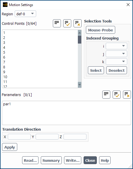
Controls (when Regular is selected from the Control Point Distribution list in the Regions tab of the Mesh Morpher/Optimizer dialog box)
- Region
selects the deformation region for which you are assigning parameters and translation directions to control points.
- Control Points
defines the control points to which you are assigning parameters and translation directions.
- Selection Tools
provides tools for selecting the control points to which you are assigning parameters and translation directions.
- Mouse-Probe
allows you to specify the Control Points by clicking in the graphics window with the mouse-probe button (which is the right mouse button, by default).
- Indexed Grouping
allows you to select the control points based on their assigned indices.
- i
allows you to select from a list of control point index numbers, which identify the location in a sequence (starting at the origin of the region) of control points along the direction-1 vector (as defined in the Regions tab of the Mesh Morpher/Optimizer dialog box).
- j
allows you to select from a list of control point index numbers, which identify the location in a sequence (starting at the origin of the region) of control points along the direction-2 vector (as defined in the Regions tab of the Mesh Morpher/Optimizer dialog box).
- k
allows you to select from a list of control point index numbers, which identify the location in a sequence (starting at the origin of the region) of control points along the direction-3 vector (as defined—though not displayed—in the Regions tab of the Mesh Morpher/Optimizer dialog box).
adds the control points that satisfy the selected index criteria (that is, the selections from the i, j, and k drop-down lists) to the list of selected Control Points.
removes the control points that satisfy the selected index criteria (that is, the selections from the i, j, and k drop-down lists) from the list of selected Control Points.
- Parameters
specifies the names of the parameters (whose values are displayed in the Parameter Values group box in the Deformation tab of the Mesh Morpher/Optimizer dialog box) that you are assigning to the Control Points. The products of the values associated with these parameters and the settings specified in the Translation Direction group box define the displacement of the control points during manual deformation.
- Translation Direction
allows you to define coefficients in the x, y, and (for 3D cases) z directions to scale the magnitude of deformation for the selected parameters. If you use a built-in optimizer, these coefficients provide the direction of the displacement of the control points and the optimizer determines the overall magnitude of displacement. Alternatively, if you manually specify the deformation or use Design Exploration in Ansys Workbench to explore multiple deformation scenarios, the values you enter in the Translation Direction group box are multiplied with the values of the Parameters (as displayed in the Parameter Values group box in the Deformation tab of the Mesh Morpher/Optimizer dialog box) to define the displacement of the control points.
- X
defines the scaling coefficient applied to the deformation parameter in the x direction.
- Y
defines the scaling coefficient applied to the deformation parameter in the y direction.
- Z
defines the scaling coefficient applied to the deformation parameter in the z direction. This number-entry box is only available for 3D cases.
saves the selections made in the Parameters selection list and the values entered in the Translation Direction group box, and assigns these parameter settings to the control points selected in the Control Points selection list.
allows you to define your motion settings by reading an ASCII text file. See Mesh Morpher/Optimizer File Formats for further details about the text file format.
- Summary
displays a summary of the saved motion settings in the console.
allows you to write your saved motion settings to an ASCII text file. See Mesh Morpher/Optimizer File Formats for further details about the text file format.
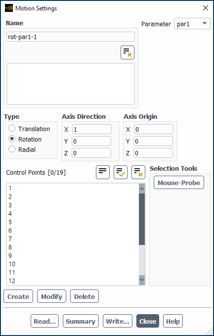
Controls (denoted by * - when Unstructured is selected from the Control Point Distribution list in the Regions tab of the Mesh Morpher/Optimizer dialog box)
- Name
provides controls for the motions you are defining. The upper text-entry box defines the name of the motion that is created when you click the button (which by default is based on the type of motion and the related parameter). The lower selection list allows you to select a motion that has already been created, in order to display the selections associated with it, or to modify or delete the motion using the or buttons, respectively.
- Parameter
allows you to select the parameter (whose value is displayed in the Parameter Values group box in the Deformation tab of the Mesh Morpher/Optimizer dialog box) for the motion.
- Type
allows you to specify the type of motion you want to define.
- Translation
specifies that the motion is a translation, based on the settings in the Direction group box.
- Rotation
specifies that the motion is a rotation about a point (for 2D) or an axis (for 3D), based on the settings in the Axis Origin group box and (for 3D cases) Axis Direction group box.
- Radial
specifies that the motion is defined radially about a point (for 2D) or an axis (for 3D), based on the settings in the Axis Origin group box and (for 3D cases) Axis Direction group box.
- Direction
allows you to define coefficients in the X, Y, and (for 3D cases) Z directions to scale the magnitude of deformation for the selected parameter. If you use a built-in optimizer, these coefficients provide the direction of the displacement of the control points and the optimizer determines the overall magnitude of displacement. Alternatively, if you manually specify the deformation or use Design Exploration in Ansys Workbench to explore multiple deformation scenarios, the values you enter in the Direction group box are multiplied with the values of the Parameter (as displayed in the Parameter Values group box in the Deformation tab of the Mesh Morpher/Optimizer dialog box) to define the displacement of the control points.
This group box is only available when Translation is selected from the Type list.
- Axis Direction
allows you to define the X, Y, and Z components of the vector about which the control points will rotate or move radially, when the selection in the Type list is Rotation or Radial, respectively. This group box is only available for 3D cases.
- Axis Origin
allows you to define the X, Y, and (for 3D cases) Z coordinates of the origin about which the control points will rotate or move radially, when the selection in the Type list is Rotation or Radial, respectively.
- Control Points*
allows you to select the control points that will undergo the motion.
- Selection Tools*
provides tools for selecting the control points that will undergo the motion.
- Mouse-Probe*
allows you to specify the Control Points by clicking in the graphics window with the mouse-probe button (which is the right mouse button, by default).
- Create
creates a new motion based on the currently displayed settings.
- Modify
modifies the saved settings for the motion selected in the lower Name selection list.
- Delete
deletes the motion selected in the lower Name selection list.
allows you to define your motion definitions by reading an ASCII text file. See Mesh Morpher/Optimizer File Formats for further details about the text file format.
- Summary*
displays a summary of the saved motion definitions in the console.
allows you to write your saved motion definitions to an ASCII text file. See Mesh Morpher/Optimizer File Formats for further details about the text file format.
![]() Setup → Boundary Conditions
→ <selected boundaries>
Setup → Boundary Conditions
→ <selected boundaries>
![]() Multi-Edit...
Multi-Edit...
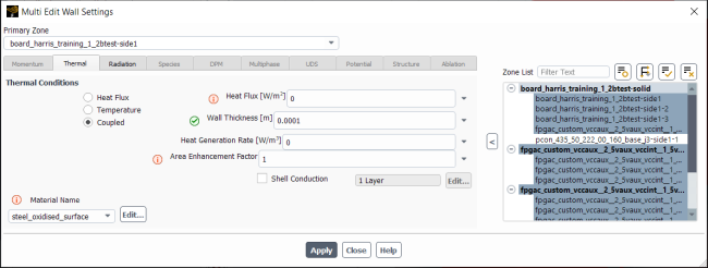
Controls
- Primary Zone
drop-down list displaying the name of the selected "primary" boundary. When the dialog box is first opened, the values of the primary zone are shown in all fields.
- Zone List
lists all of the zones that are compatible for multi-editing with the primary zone. The selected zones are the ones that will be modified on .
applies the settings marked with the
 icon to the selected boundaries in the Zone
List.
icon to the selected boundaries in the Zone
List.
 indicates that the value of this setting varies between the
selected boundaries in the Zone List.
indicates that the value of this setting varies between the
selected boundaries in the Zone List.- indicates that the displayed value will be applied to the selected
boundaries in the Zone List when you click
.
Refer to Editing Multiple Boundary Conditions at Once for additional information about this functionality. Note that while this image shows the Multi Edit Velocity Wall Settings dialog box, the functionality that is specific to multi-editing is consistent across the different multi-edit dialog boxes. For information on specific settings of boundary conditions, refer to Boundary Conditions Task Page (which contains descriptions of each boundary's dialog box), and Boundary Conditions.
![]() Solution → Reports
→ File...
Solution → Reports
→ File...
Click in the Report File Definitions dialog box to open the New Report File dialog box.
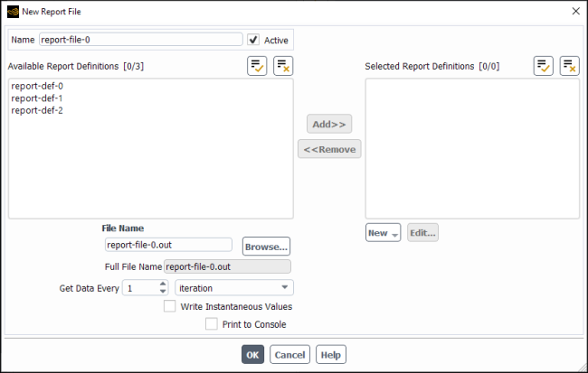
Controls
- Name
editable field displaying the name of the report file.
- Active
check box (enabled by default) that determines if the file is written during the solution calculation.
- Available Report Definitions
lists all of the existing report definitions not currently part of this report file.
- Add>>
moves the selected report definition(s) to the Selected Report Definitions list.
- <<Remove
moves the selected report definition(s) to the Available Report Definitions list.
- File Name
allows you to specify the name used when the file is saved.
- Browse...
opens the Select File dialog box, allowing you to specify the location where the report file will be saved.
- Full File Name
displays the name and location of the report file once it has been saved.
- Get Data Every
indicates the frequency that the report definition data is written to the file. The default value of 1 allows you to write to the file at every iteration or time-step. If you select flow-time, then you must specify the frequency for writing the file in units of time. Time-step and flow-time are only a valid choices when you are calculating unsteady flow.
- Print to Console
indicates whether or not the contents of the report file are printed to the console at the frequency specified in the Get Data Every field.
- Selected Report Definitions
lists all of the existing report definitions currently included in this report file.
- New
drop-down list allowing you to create new report definitions (surface, volume, force, flux, mesh, aeromechanics, dpm, expression, and user-defined).
- Edit...
allows you to modify the highlighted report definition in the Selected Report Definition list.
![]() Solution → Reports
→ Plot...
Solution → Reports
→ Plot...
Click in the Report Plot Definitions dialog box to open the New Report Plot dialog box.
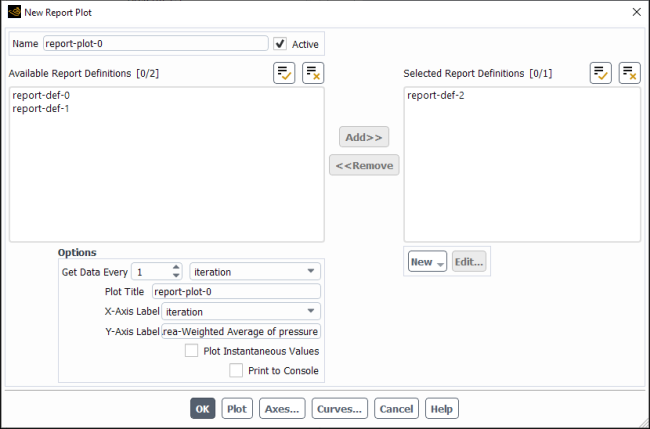
Controls
- Name
editable field displaying the name of the report plot.
- Active
check box (enabled by default) that determines if the plot is plotted during the solution calculation.
- Available Report Definitions
lists all of the existing report definitions not currently part of this report plot.
- Add>>
moves the selected report definition(s) to the Selected Report Definitions list.
- <<Remove
moves the selected report definition(s) to the Available Report Definitions list.
- Options
- Get Data Every
indicates the frequency that the report definition data is plotted. The default value of 1 allows you to write to the file at every iteration or time-step. If you select flow-time, then you must specify the frequency for plotting the data in units of time. Time-step and flow-time are only a valid choices when you are calculating unsteady flow.
- Plot Title
provide a title for the plot.
- X-Axis Label
choose whether the X-axis is flow-time or time-step.
- Y-Axis Label
enter a label for the Y-axis.
- Print to Console
indicates whether or not the contents of the report plot are printed to the console at the frequency specified in the Get Data Every field.
- Selected Report Definitions
lists all of the existing report definitions currently included in this report plot.
- New
drop-down list allowing you to create new report definitions (surface, volume, force, flux, mesh, aeromechanics, dpm, expression, and user-defined).
- Edit...
allows you to modify the highlighted report definition in the Selected Report Definition list.
- Curves...
opens the Curves Dialog Box.
- Axes...
opens the Axes Dialog Box.
The Objective Function Definition dialog box allows you to specify the format of the objective function that will be minimized by the mesh morpher/optimizer and (when it is a customized function of output parameters) to define the objective function. See Using the Mesh Morpher/Optimizer for details about using this dialog box.
The Objective Function Definition dialog box is opened from the Mesh Morpher/Optimizer Dialog Box.
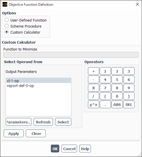
Controls
- Options
contains options for the format of the objective function.
- User-Defined Function
specifies that the objective function is provided via a user-defined function.
- Scheme Procedure
specifies that the objective function is provided via a Scheme source file. This option is not available if newuoa is selected from the Optimizer drop-down list in the Optimizer tab of the Mesh Morpher/Optimizer dialog box.
- Custom Calculator
specifies that the objective function is based on output parameters, and is defined by the controls in the Custom Calculator group box. This option is not available if newuoa is selected from the Optimizer drop-down list in the Optimizer tab of the Mesh Morpher/Optimizer dialog box.
- Custom Calculator
allows you to define the objective function. This group box is only available when Custom Calculator is selected from the Options list.
- Function to Minimize
displays the objective function defined by the controls in the Custom Calculator group box.
- Select Operand from
allows you to include output parameters in the definition of the objective function.
- Output Parameters
provides a list of available output parameters, which can be included in the definition of the objective function.
- Parameters...
opens the Parameters Dialog Box, which you can use to create additional output parameters.
- Refresh
updates the Output Parameters list, so that all available output parameters are displayed.
- Select
enters the output parameter that is currently selected in the Output Parameters list in the Function to Minimize field.
- Operators
allows you to include calculator operators in the definition of the objective function. Clicking a button in this group box causes the appropriate symbol to appear in the Function to Minimize field.
- Apply
saves the custom objective function (displayed in the Function to Minimize field) as part of the case file.
- Clear
deletes all of the text in the Function to Minimize field.
The Optimization History Monitor dialog box allows you to plot and/or record optimization history data, that is, how the value of the objective function (defined using the Mesh Morpher/Optimizer Dialog Box) varies with each design stage produced by the mesh morpher/optimizer. See Using the Mesh Morpher/Optimizer for details about using this dialog box.
The Optimization History Monitor dialog box is opened from the Mesh Morpher/Optimizer Dialog Box.
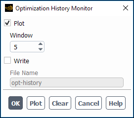
Controls
- Plot
enables the plotting of the optimization history data in the graphics window.
- Window
optimization history data are automatically displayed in the appropriate window, so changing the number in the Window field will not modify the display location.
- Write
enables the saving of the optimization history data to a file (with the name specified in File Name).
- File Name
specifies the name of the file to which the optimization history data is written. This text-entry box is only available when the Write option is enabled.
- Plot (button)
displays an XY plot of the optimization history data generated during the last calculation. Note that no plot will be displayed if the data was discarded using the button.
- Clear
discards the optimization history data, including the associated files. Each of these actions must be confirmed in a Question Dialog Box.
The Parallel Connectivity dialog box prints the connectivity of the selected compute node. See Checking Network Connectivity for details.
![]() Parallel → Network → Connectivity...
Parallel → Network → Connectivity...
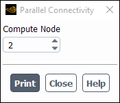
Controls
- Compute Node
indicates the compute node ID for which connectivity information is desired.
prints information (in the console window) about the network connectivity for the selected compute node.
The Parameter Bounds dialog box allows you to limit how much each parameter is allowed to deform when using the mesh morpher/optimizer. See Using the Mesh Morpher/Optimizer for details about using this dialog box.
The Parameter Bounds dialog box is opened from the Mesh Morpher/Optimizer Dialog Box.
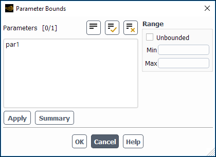
Controls
- Parameters
selects the parameters (created using the Deformation tab of the Mesh Morpher/Optimizer Dialog Box) for which you are defining bounds.
- Range
allows you to specify the bounds.
- Unbounded
allows you to specify whether the selected Parameters are unbounded.
- Min, Max
allows you to set the minimum and maximum values allowed for the selected Parameters when the Unbounded option is disabled.
- Apply
saves the bounds for the currently selected Parameters.
- Summary
displays a summary of all of the saved parameter bounds in the console.
The Particle Tracks dialog box controls the generation and display of discrete phase particles. See Displaying of Trajectories for details about the items below.
![]() Results → Graphics
→ Particle Tracks → New...
Results → Graphics
→ Particle Tracks → New...
Note:
The "global"/non-persistent form of graphics objects is hidden by default. If this interrupts your workflow, you can make them available by enabling the Expose legacy non-persistent graphics option in the Graphics branch of Preferences (accessed via File>Preferences...).
(When you click Edit... instead of New..., it opens the "global"/non-persistent version of the Particle Tracks dialog box. This version of the dialog box does not have a Name field and it is not saved with the case file.
You are encouraged to use the persistent version that is accessed by clicking New....
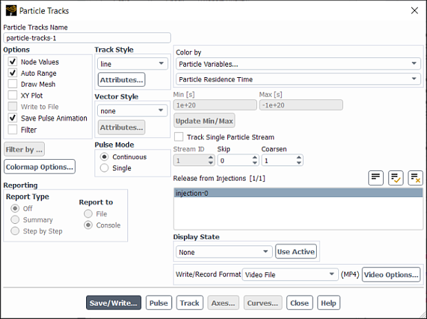
Controls
- Particle Tracks Name
is the name for a particle tracks definition. You can specify a name or use the default name
particle-tracks-. This control appears only for particle tracks definitions.id- Options
contains the options described below:
- Node Values
specifies that node values should be interpolated to compute the scalar field at a particle location. This option is turned on by default. See Choosing Node or Cell Values for details.
- Auto Range
specifies that the minimum and maximum values of the scalar field will be the limits of that field. If this option is not selected, you can enter Min and Max values manually. These values determine the range of the color scale.
- Draw Mesh
toggles between displaying and not displaying the mesh. The Mesh Display Dialog Box is opened when Draw Mesh is selected.
- XY Plot
enables the display of an XY plot along the particle trajectories for steady particle tracking and at the current particle locations for unsteady tracking. When this option is selected, the Display push button will change to Plot.
- Write to File
(available only when XY Plot is on) activates the file-writing option. When this option is selected, the Plot push button will change to Write.... Clicking on the Write... button will open The Select File Dialog Box, in which you can specify a name and save a file containing the XY plot data. The format of this file is described in XY Plot File Format.
- Save Pulse Animation
allows you to save a video or picture files of the pulse animation. When this option is enabled, an additional field for Write/Record Format appears, allowing you to specify how the pulse animation will be saved. Clicking opens The Select File Dialog Box where you can specify a name and save the video or picture files.
A Continuous pulse video file will be 5 seconds long, while a Single pulse video will be one full cycle.
- Filter
when selected, the Filter by... button becomes available.
- Filter by...
opens the Particle Filter Attributes Dialog Box where you can specify how you would like to filter the particles being displayed. This button is available when Filter is selected in the Options group box.
- Colormap Options...
opens the Colormap Dialog Box, allowing you to customize the colormap for this graphics object.
- Reporting
allows you to specify how you would like to report particle tracks.
- Report Type
controls the type of trajectory-fate reports to be displayed.
- Off
disables reporting of trajectory fates.
- Summary
enables summary reports of trajectory fates. See Particle Tracking Statistics for details.
- Step by Step
enables the step-by-step reporting of trajectories. This item will not appear if you have requested unsteady tracking in the Discrete Phase Model Dialog Box. See Step-by-Step Reporting of Trajectories for details.
- Current Positions
enables the reporting of the positions and velocities of all particles that are in the domain at the current time. This item appears only when unsteady tracking has been requested in the Discrete Phase Model Dialog Box. See Reporting of Current Positions for Unsteady Tracking for details.
- Report to
indicates the destination of the trajectory report.
- File
enables the writing of the trajectory report to a file. When this option is enabled, the Track button will become the Write... button.
- Console
enables the display of the trajectory report information in the console window.
- Significant Figures
controls the number of significant figures used when a Step by Step or Current Positions report is selected.
- Sample File Format
allows you to generate a file containing particle current positions in the same file format that is used for particle sampling. This item is available only for unsteady particle tracking when Current Positions and File are selected in the Reporting group box. See Reporting of Current Positions for Unsteady Tracking for details.
- Reporting Variables...
opens the Reporting Variables Dialog Box that contains a list from which you can select the scalar field to be used to color the particle tracks.
- Track Style
sets the trajectory style. Trajectories can be displayed as lines, ribbons, spheres, cylinders, or a set of points. Pulsing can be done only on point or line styles.
- Attributes...
opens the Track Style Attributes Dialog Box, Particle Sphere Style Attributes Dialog Box, or the Ribbon Attributes Dialog Box, depending on the selected Track Style. These dialog boxes allow you to set the attributes for the chosen trajectory style.
- Vector Style
sets the trajectory vector style. You can display the trajectories vectors in three different ways: vector, centered-vector, and centered-cylinder. All three styles are demonstrated in Controlling the Vector Style of Particle Tracks.
- Attributes...
opens the Particle Vector Style Attributes Dialog Box.
- Pulse Mode
specifies either a single or continuous release of particles that follow the trajectories, starting at the release surface, when you use the Pulse button to animate the trajectories.
- Continuous
sets the pulse mode to continuously release particles from the initial positions.
- Single
sets the pulse mode to release a single wave of particles.
The Pulse Mode is used only when particles are being Pulsed.
- Y Axis Function
contains a list of solution variables that can be used for the
 axis of the plot.
This item appears when the XY Plot option is turned on.
- X Axis Function
contains a list of functions for the X-axis of the plot. You can plot the quantity selected in the Y Axis Function drop-down list as a function of the Time elapsed along the trajectory, or the Path Length along the trajectory.
This item appears when the XY Plot option is turned on.
- Phase
(Multiphase only) specifies the phase where the postprocessing operations are being applied.
- Min/Max
display the values to which the lower and upper ends of the color scale map. If you are using the Auto Range option, these values will be automatically computed when you click Compute. If you are not using Auto Range, you can enter values manually.
- Update Min/Max
computes the Min and Max for the field chosen in Color by.
- Track PDF Transport Particles
enables the tracking of PDF transport particles. This item is available only when the composition PDF transport model is enabled.
- Free Stream Particles
enables the tracking of free stream particles. Note that this option is available only when the Lagrangian wallfilm model is enabled in the wall boundary conditions dialog box, under the DPM tab.
- Wall Film Particles
enables the tracking of wall film particles. Note that this option is available only when the Lagrangian wallfilm model is enabled in the wall boundary conditions dialog box, under the DPM tab.
- Track Single Particle Stream
enables the tracking of a single particle stream in the selected injection, instead of all the streams in that injection. See Displaying of Trajectories for details.
- Stream ID
specifies the particle stream to be tracked when the Track Single Particle Stream option is enabled.
- Skip
allows you to "thin" or "sample" the particles that are displayed.
- Coarsen
reduces the plotting time by reducing the number of points that are plotted for a given trajectory in any cell. This is valid only for steady-state cases.
- Release from Injections
selects the injections from which to release particles. You must select at least one injection before any particles can be released.
- Display State
specifies the display state that is associated with this graphics object.
- drop-down list of display states
selectable list of all the existing display states associated with this case.
creates a display state that matches the settings of the active graphics window and assigns it to this graphics object (this association is only saved after you click ).
- Write/Record Format
(only present when Save Pulse Animation is enabled) drop-down list specifying whether you are saving the pulse animation as a video file or as picture files. The default formats are shown in parenthesis next to the field.
(only present when Save Pulse Animation is enabled and Video File is selected for Write/Record Format) opens the Video Options Dialog Box.
(only present when Save Pulse Animation is enabled and Picture Files is selected for Write/Record Format) opens the Save Picture Dialog Box.
- Display
displays the particle trajectories and generates a trajectory report in the console window (if requested) for steady particle tracking. For unsteady particle tracking, only the current particle locations will be shown.
- Save/Display
displays the particle tracks (steady tracking) or the current particle locations (unsteady tracking) in the active graphics window and saves the particle track definition. This button appears only for particle track definitions and replaces the Display button.
- Plot
displays an XY plot along the particle trajectories. This button replaces the Display button when the XY Plot option is turned on.
- Write...
opens The Select File Dialog Box, in which you can save the XY plot data or trajectory report to a file. This button replaces the Plot button when the Write to File option is turned on, or the Track button when the File option is selected under Report to.
- Pulse
animates the position of particles. If Pulse Mode is set to Continuous, particles are reintroduced at the seed positions repeatedly. If the mode is Single, a single wave of particles moves through the domain. Pulse is not available for unsteady tracking.
The label of this button changes to Stop ! when the animation is in progress. Click Stop ! to stop pulsing (and the label goes back to Pulse).
- Track
computes the particle trajectories and generates any reports without displaying the trajectories in the graphics window.
- Axes...
opens the Axes Dialog Box, which allows you to customize the XY plot axes. This item appears when the XY Plot option is turned on.
- Curves...
opens the Curves Dialog Box, which allows you to customize the curves used in the XY plot. This item appears when the XY Plot option is turned on.
The Partition Surface dialog box allows you to create a surface defined by the boundary of two adjacent mesh partitions. See Partition Surfaces for details about the items below.
![]() Domain → Surface
→ Create → Partition...
Domain → Surface
→ Create → Partition...
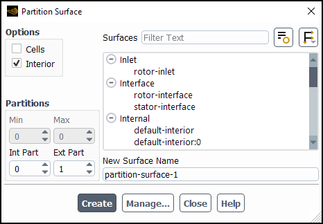
Controls
- Options
contains check buttons that allow you to choose interior or exterior faces or cells to be contained in the partition surface.
- Cells
specifies, when enabled, that the partition surface will consist of cells (either interior or exterior, depending on the status of the Interior check button) that lie on the partition boundary. When this option is disabled, the faces on the boundary between partitions will make up the partition surface. Depending on the status of the Interior check button, the faces will reflect data values for the interior or exterior cells.
- Interior
toggles between interior and exterior cells. If the partition surface consists of faces instead of cells, Interior specifies for which cells data will be displayed on the faces. When this option is enabled, interior cells (cells that are on the Int Part side of the partition boundary) will make up the partition surface. When it is disabled, the partition surface will consist of exterior cells (cells that are on the Ext Part side of the partition boundary).
- Partitions
contains information about which partitions are under consideration. The boundary that defines the partition surface is the boundary between the Int Part and the Ext Part. If there are more than two mesh partitions, each interior partition will share boundaries with several exterior partitions. By setting the appropriate values for Int Part and Ext Part, you can create surfaces for any of these boundaries.
- Min/Max
indicates the minimum and maximum ID numbers of the mesh partitions. The minimum is always zero, and the maximum is one less than the number of processors.
- Int Part
indicates the ID number of the interior partition (that is, the partition under consideration).
- Ext Part
indicates the ID number of the bordering partition.
- Surfaces
displays an informational list of existing surfaces.
- New Surface Name
designates the name of the new surface. The default is the concatenation of the surface type and an integer which is the new surface ID.
creates the surface.
opens the Surfaces Dialog Box in which you can rename and delete surfaces and determine their sizes.
The Partitioning and Load Balancing dialog box allows you to partition the mesh into separate clusters of cells for separate processors on a parallel computer. See Partitioning the Mesh Manually and Balancing the Load for details.
The Partitioning and Load Balancing dialog box also allows you to enable and control Ansys Fluent’s load balancing feature. Load balancing will automatically detect and analyze parallel performance, and redistribute cells between the existing compute nodes to optimize it. See Load Balancing for more information about load balancing.
![]() Parallel → General → Partitioning/Load Balancing...
Parallel → General → Partitioning/Load Balancing...
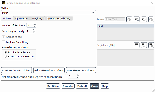
Controls
- Method
contains a drop-down list of the recursive partition methods that can be used to create the mesh partitions. The choices include the Cartesian Axes, Cartesian Strip, Cartesian X-Coordinate, Cartesian Y-Coordinate, Cartesian Z-Coordinate, Cartesian R Axes, Cartesian RX-Coordinate, Cartesian RY-Coordinate, Cartesian RZ-Coordinate, Cylindrical Axes, Cylindrical R-Coordinate, Cylindrical Theta-Coordinate, Cylindrical Z-Coordinate, Metis, Polar Axes, Polar R-Coordinate, Polar Theta-Coordinate, Principal Axes, Principal Strip, Principal X-Coordinate, Principal Y-Coordinate, Principal Z-Coordinate, Spherical Axes, Spherical Rho-Coordinate, Spherical Theta-Coordinate, and Spherical Phi-Coordinate techniques, which are described in Mesh Partitioning Methods.
- Options
tab
- Number of Partitions
defines the desired number of mesh partitions. This usually matches the number of processors available for parallel computing.
- Reporting Verbosity
specifies the amount of information to be reported in the text (console) window during the partitioning. With the default value of 1, Fluent will print the number of partitions created, the number of bisections performed, the time required for the partitioning, and the minimum and maximum cell, face, interface, and face-ratio variations. (See Interpreting Partition Statistics for details.) If you increase the Reporting Verbosity to 2, the partition method used, the partition ID, number of cells, faces, and interfaces, and the ratio of interfaces to faces for each partition will also be printed in the console window. If you decrease the Reporting Verbosity to 0, only the number of partitions created and the time required for the partitioning will be reported.
- Across Zones
allows partitions to cross zone boundaries (the default). If turned off, it will restrict partitioning to within each cell zone. This is recommended only when cells in different zones require significantly different amounts of computation during the solution phase, for example if the domain contains both solid and fluid zones.
- Laplace Smoothing
enables the Laplace smoothing method, which can be used to prevent partition boundaries from passing through regions of high aspect ratio cells. This can improve the convergence and scalability of the flow and conjugate heat transfer computations for cases with regions of highly stretched cells.
- Cutoff Aspect Ratio
controls the threshold for the Laplace smoothing method.
- Reordering Method
is used to optimize parallel performance
- Architecture Aware
is the default option and it accounts for the system architecture and network topology in remapping the partitions to the processors.
- Reverse Cuthill-McKee
minimizes the bandwidth of the compute-node connectivity matrix (the maximum distance between two connected processes) without incorporating the system architecture.
- Optimization
tab contains options for enabling schemes to optimize the partitions created by the selected partition method. In addition, the optimization scheme will be applied until appropriate criteria are met, or the maximum number of iterations have been run. If the Iterations counter is set to 0, the optimization scheme will be applied until completion, without limit on the maximum number of iterations.
- Merge
attempts to decrease the number of interfaces by eliminating orphan cell clusters (an orphan cluster is a group of connected cells whose members each have at least one face coincident with an interface boundary).
- Smooth
attempts to minimize the number of interfaces by sacrificing cells on the partition boundary to the neighboring partition to reduce the partition boundary surface area.
- Pre-Test
instructs Fluent to test all coordinate directions and choose the one which yields the fewest partition interfaces for the final bisection. Note that this option is available only when you choose Principal Axes or Cartesian Axes as the partitioning method.
- Weighting
tab allows you to set the appropriate weights, prior to partitioning the mesh.
- Weight Types
allows you to turn on/off a specific weight. Weight types include: Faces per Cell (enabled by default, with additional weighting of 2), Solid Zones (available and enabled by default only if solid cell zones are defined); VOF (available only if the volume of fluid multiphase model is turned on); DPM (available only for discrete phase simulations with injections defined), where you can specify Hybrid Optimization; and ISAT.
- User Specified
allows you to specify that Ansys Fluent timers set the weight scaling (by not enabling the check box), or to modify the value yourself (by enabling the check box and entering a numerical value in the Value field.)
- Value
allows you to enter a user-specified numerical value to modify the weighting set by the Ansys Fluent timers. Note that for VOF, DPM, and ISAT, this value is not relevant when using model-weighted partitioning.
- Dynamic Load Balancing
tab allows you to set load balancing thresholds and intervals.
- Physical Models
allows you to set thresholds and intervals for the simulation’s physical models.
- Threshold
is a percentage and depending on the value, load balancing will occur if the load imbalance is greater than the value entered.
- Interval
allows you to specify the desired interval for load balancing cycles, in terms of number of iterations. When a value of 0 is specified, Ansys Fluent will internally determine the best value to use, initially using an interval of 25 iterations. You can override this behavior by specifying a nonzero value. Ansys Fluent will then attempt to perform load balancing after every N iterations, where N is the specified Balance Interval.
- Dynamic Mesh
allows you to set load balancing threshold and interval values for your dynamic mesh. This option is only available when the dynamic mesh model is enabled.
- Auto
allows a percentage of interface faces and loads to be automatically traced.
- Threshold
is a percentage and depending on the value, load balancing will occur if the load imbalance is greater than the value entered.
- Interval
allows you to specify the desired interval for load balancing cycles, in terms of number of iterations. When a value of 0 is specified, Ansys Fluent will internally determine the best value to use, initially using an interval of 25 iterations. You can override this behavior by specifying a nonzero value. Ansys Fluent will then attempt to perform load balancing after every N iterations, where N is the specified Balance Interval.
- Mesh Adaption
allows you to set threshold values for mesh adaption.
- Threshold
is a percentage and depending on the value, load balancing will occur if the load imbalance is greater than the value entered.
- Zones
contains a list of cell zones. Partitioning will be applied to cells in zones selected from this list.
- Registers
contains a list of cell registers that have been created using the adaption tools. You can restrict partitioning to a group of cells by selecting a register containing the cells. See Partitioning Within Zones or Registers for details.
prints the partition ID, number of cells, faces, and interfaces, and the ratio of interfaces to faces for each active partition (see Checking the Partitions for information about active partitions) in the console. In addition, it prints the minimum and maximum cell, face, interface, and face-ratio variations.
prints the partition ID, number of cells, faces, and interfaces, and the ratio of interfaces to faces for each stored partition (see Checking the Partitions for information about stored partitions) in the console. In addition, it prints the minimum and maximum cell, face, interface, and face-ratio variations.
allows you to set a value that assigns selected Zones and/or Registers to a specific partition ID. A region or zone is marked before setting the marked cells to one of the partition IDs.
allows you to make the stored cell partitions the active cell partitions in a parallel session. The active cell partition is used for the current calculation, while the stored cell partition (the last partition performed) is used when you save a case file.
subdivides the mesh into the selected number of partitions using the prescribed method and optimization(s).
sets all controls to their default values, as assigned by Ansys Fluent. After execution, the Default button becomes the Reset button.
resets the fields to their most recently saved values (that is, the values before Default was selected). After execution, the button becomes the button.
The Pathlines dialog box controls the generation and display of pathlines. See Displaying Pathlines for details about the items below.
![]() Results → Graphics
→ Pathlines → New...
Results → Graphics
→ Pathlines → New...
Note:
The "global"/non-persistent form of graphics objects is hidden by default. If this interrupts your workflow, you can make them available by enabling the Expose legacy non-persistent graphics option in the Graphics branch of Preferences (accessed via File>Preferences...).
(When you click Edit... instead of New..., it opens the "global"/non-persistent version of the Pathlines dialog box. This version of the dialog box does not have a Name field and it is not saved with the case file.
You are encouraged to use the persistent version that is accessed by clicking New....
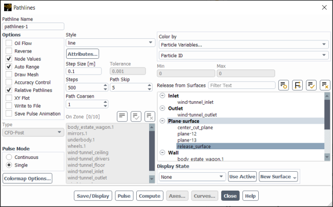
Controls
- Pathline Name
is the name for a pathline definition. You can specify a name or use the default name
pathline-. This control appears only for pathline definitions.id- Options
contains the options described below:
- Oil Flow
toggles between regular pathlines and oil-flow pathlines. When this option is selected, pathlines are constrained to lie on the zone(s) selected in the On Zone list.
- Reverse
specifies that each particle’s path is traced back in time. This option is turned off by default.
- Node Values
specifies that node values should be interpolated to compute the scalar field at a particle location. This option is turned on by default. See Choosing Node or Cell Values for details.
- Auto Range
specifies that the minimum and maximum values of the scalar field will be the limits of that field. If this option is not selected, you can enter Min and Max values manually. These values determine the range of the color scale.
- Draw Mesh
when enabled opens the Mesh Display Dialog Box where you can specify how to display your mesh.
- Accuracy Control
allows you to specify tolerance to control the pathlines accuracy.
- Relative Pathlines
allows you to display the pathlines relative to the rotating reference frame.
- XY Plot
enables the display of an XY plot along the pathline trajectories. When this option is selected, the Display push button will change to Plot.
- Write to File
activates the file-writing option. When this option is enabled, the Type option becomes active and the Save/Plot button changes to Save/Write.... Clicking Save/Write... opens The Select File Dialog Box where you can specify a name and save a file containing the XY plot data. The format of this file is described in XY Plot File Format.
- Save Pulse Animation
allows you to save a video or picture files of the pulse animation. When this option is enabled, an additional field for Write/Record Format appears, allowing you to specify how the pulse animation will be saved. Clicking opens The Select File Dialog Box where you can specify a name and save the video or picture files.
A Continuous pulse video file will be 5 seconds long, while a Single pulse video will be one full cycle.
- Type
specifies the type of the file you want to write.
- CFD-Post
allows you to write the file in CFD-Post compatible format, which can be read in CFD-Post.
- Fieldview
allows you to write the file in FIELDVIEW format, which can be read in FIELDVIEW.
- Geometry
allows you to write the file in
.iblformat, which can be read in GAMBIT.- EnSight
allows you to write the file in
.encasformat, which can be read in EnSight.
- Pulse Mode
specifies either a single or continuous release of particles that follow the pathlines, starting at the release surface, when you use the Pulse button to animate the pathlines.
- Continuous
sets the pulse mode to continuously release particles from the initial positions.
- Single
sets the pulse mode to release a single wave of particles.
The Pulse Mode is used only when particles are being pulsed.
- Colormap Options...
opens the Colormap Dialog Box, allowing you to customize the colormap for this graphics object.
- Style
sets the pathline style. Pathlines can be displayed as lines, ribbons, spheres, cylinders, or a set of points. The ribbon style also uses the Twist By field and the TwistFactor value (specified in the Ribbon Attributes Dialog Box). Pulsing can be done only on point or line styles.
- Attributes...
opens the Path Style Attributes Dialog Box or the Ribbon Attributes Dialog Box, depending on the selected Style. These dialog boxes allow you to set the attributes (ribbon width, marker size, cylinder radius, twist-by field, and so on) for the chosen pathline style.
- Step Size
sets the interval used for computing the next position of a particle. This is in units of length. Particle positions are always computed when they enter/leave a cell. If you specify a very large size, the particle positions at entry/exit of each cell will still be computed (and displayed).
- Tolerance
allows you to control the error when using large time step sizes for the calculation. This is available when Accuracy Control is selected under Options.
- Steps
sets the maximum number of steps a particle can advance. A particle’s path may also end if it leaves the domain.
- Path Skip
allows you to "thin" or "sample" the pathlines that are displayed. See “Thinning” Pathlines for details.
- Path Coarsen
reduces the time and the number of points plotted in a pathline. Coarsening factor of ’n’ will result in plotting of each ’n’th point for a given pathline in each cell.
- On Zone
contains a list from which you can select the zone(s) on which the particles are constrained to lie. This list is activated only when the Oil Flow option is selected.
- Track in Phase
(for the Eulerian Multiphase model only) allows you to select the phase or the mixture of all phases for tracking particle pathlines.
- Color by
contains a list from which you can select the scalar field to be used to color the pathlines. The default is Particle ID, a unique ID for each particle.
- Y Axis Function
contains a list of solution variables that can be used for the
 axis of the plot.
This item appears when the XY Plot option is turned on.
- X Axis Function
contains a list of functions for the
 axis of the plot. You can plot the quantity selected in the
Y Axis Function drop-down list as a function of the
Time elapsed along the trajectory, or the Path
Length along the trajectory.
axis of the plot. You can plot the quantity selected in the
Y Axis Function drop-down list as a function of the
Time elapsed along the trajectory, or the Path
Length along the trajectory.This item appears when the XY Plot option is turned on.
- Phase
(Multiphase only) specifies the phase where the postprocessing operations are being applied.
- Min/Max
display the values to which the lower and upper ends of the color scale map. If you are using the Auto Range option, these values will be automatically computed when you click Compute. If you are not using Auto Range, you can enter values manually.
- Release from Surfaces
selects the surfaces from which to release particles. You must select at least one surface before any particles can be released.
- Display State
specifies the display state that is associated with this graphics object.
- drop-down list of display states
selectable list of all the existing display states associated with this case.
creates a display state that matches the settings of the active graphics window and assigns it to this graphics object (this association is only saved after you click ).
- New Surface
is a drop-down list button that contains a list of surface options:
- Point
opens the Point Surface Dialog Box.
- Line/Rake
opens the Line/Rake Surface Dialog Box.
- Plane
opens the Plane Surface Dialog Box.
- Quadric
opens the Quadric Surface Dialog Box.
- Iso-Surface
opens the Iso-Surface Dialog Box.
- Iso-Clip
opens the Iso-Clip Dialog Box.
- Structural Point
opens the Structural Point Surface Dialog Box.
- Write/Record Format
(only present when Save Pulse Animation is enabled) drop-down list specifying whether you are saving the pulse animation as a video file or as picture files. The default formats are shown in parenthesis next to the field.
(only present when Save Pulse Animation is enabled and Video File is selected for Write/Record Format) opens the Video Options Dialog Box.
(only present when Save Pulse Animation is enabled and Picture Files is selected for Write/Record Format) opens the Save Picture Dialog Box.
- EnSight Encas File Name
allows you to specify a.encas file name if you selected EnSight under Type.
- Browse...
opens The Select File Dialog Box where you can select the
.encasfile.- Time Steps For EnSight Export
allows you to set the number of time levels that are available for animation in EnSight.
- Display
displays the pathlines in the active graphics window.
- Save/Display
plots the pathlines in the active graphics window and saves the pathline definition. This button appears only for pathline definitions and replaces the Display button.
- Plot
displays an XY plot along the pathline trajectories. This button replaces the Display button when the XY Plot option is turned on.
- Write...
opens The Select File Dialog Box, in which you can save the XY plot data to a file. This button replaces the Plot button when the Write to File option is turned on.
- Pulse
animates the position of particles. If Pulse Mode is set to Continuous, particles are reintroduced at the seed positions repeatedly. If the mode is Single, a single wave of particles moves through the domain.
The label of this button changes to Stop ! when the animation is in progress. Click Stop ! to stop pulsing (and the label goes back to Pulse).
- Compute
computes the Min and Max for the field chosen in Color by.
- Axes...
opens the Axes Dialog Box, which allows you to customize the XY plot axes. This item appears when the XY Plot option is turned on.
- Curves...
opens the Curves Dialog Box, which allows you to customize the curves used in the XY plot. This item appears when the XY Plot option is turned on.
The PCB Model dialog box allows you to model printed circuit boards (PCB) that vary considerably due to their layered construction and highly variable metal fraction at any particular location. See Thermal Analysis of Printed Circuit Boards for details about the items below.
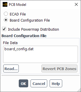
Controls
- Board Configuration File
contains the options for the PCB model described below:
- Read..
reads the board configuration file produced by Ansys Icepak.
- File Data
displays the name of the board configuration file.
- Include Powermap Distribution
select to include powermap distribution as part of the analysis from additional files generated by Ansys Icepak.
The Plane Surface dialog box allows you to interactively create one or more planar surfaces that cut through the domain. See Plane Surfaces for details about the items below.
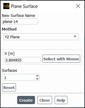
Controls
- New Surface Name
designates the name of the new surface. The default is the concatenation of the surface type and an integer which is the new surface ID.
- Name Format
[Creating multiple YZ, ZX, XY planes only] indicates how Fluent will name the surfaces.
The field will look something like
plane-x={x:+.6f}. This naming format results in plane names that reflect the coordinates of the plane. For example, if you create three YZ planes, with a spacing of 0.05m, starting from X=2.325m, the planes will be namedplane-x=+2.325000,plane-x=+2.375000, andplane-x=+2.425000. You can control how many significant digits are included in the plane name by varying the value represented by6in the example name format. Thefin the example name indicates that the output is a float. Changing thefto aneresults in the coordinate being represented as an exponential.
- Method
displays the selected plane creation method.
- YZ Plane
create a plane surface in the YZ plane.
- ZX Plane
create a plane surface in the ZX plane.
- XY Plane
create a plane surface in the XY plane.
- Point and Normal
create a plane surface based on a point and its normal. Normal can optionally be computed from a surface or the current view.
- Three Points
create a plane surface based on three points.
- Normal
settings related to specifying the normal direction for a Point and Normal plane surface.
- iX, iY, iZ
designates the coordinates of the end point of the normal vector (the start point being 0, 0, 0).
- Compute from Surface
computes values for the Normal based on the surface selected from the drop-down above.
- Compute from View Plane
computes values for the Normal based on the current view orientation in the graphics window.
- Options
contains options for defining the plane surface.
- Bounded
enables the creation of a bounded parallelepiped, 3 of whose 4 corners are the 3 points that define the plane equation (or the 4 corners of the Plane Tool).
- Sample Points
enables the specification of a point density along the 2 directions (of the parallelepiped). This creates a uniformly distributed set of points on the plane. (This item is available only when the Bounded option is enabled.)
- Sample Density
specifies the density of points when the Sample Points option is enabled.
- Edge 1, Edge 2
sets the point density along the two directions of the plane. (Edge 1 extends from point 0 to point 1, and edge 2 extends from point 1 to point 2.)
- Select with Mouse
allows you to select points with the mouse. You can select endpoints by clicking on locations in the active window with the mouse-probe button. (See Controlling the Mouse Button Functions for information about setting mouse button functions.)
- Point 1
designates the coordinates of the first point.
- Point 2
designates the coordinates of the second point.
- Point 3
designates the coordinates of the third point.
- Surfaces
lists the number of surfaces that will be created at once.
- Spacing
specifies the distance between surfaces.
- Reset
resets the plane tool to its default position.
- Create
creates the surface.
The Point Surface dialog box allows you to interactively create point surfaces (surfaces containing a single data point). See Point Surfaces for details about the items below.
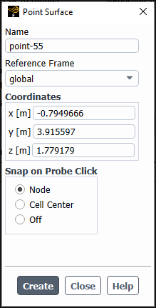
Controls
- Name
designates the name of the new surface. The default is the concatenation of the surface type and an integer which is the new surface ID.
- Reference Frame
allows you to specify a local reference frame (if defined) for the point surface.
- Coordinates
designates the coordinates of the point in the surface (x0, y0, z0).
- Snap on Probe Click
updates the coordinates of the point to the closest Node or Cell Center when you click on the model in the graphics window using the probe tool—that is, either by right-clicking or setting the left-mouse-button to probe (
 ).
).You can disable automatic snapping by selecting Off.
- Create
creates the surface.
The Quadric Surface dialog box allows you to interactively define quadric functions and create surfaces from them. Lines and circles are commonly used types of quadric functions, so additional support is provided for defining them. See Quadric Surfaces for details about using the items below.
Important: Note that your inputs for the quadric function must be in SI units.
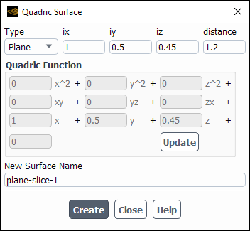
Controls
- Type
selects the type of quadric function. Presently, you may select Line/Plane, Circle/Sphere or a general Quadric. Some of the control buttons take on different meanings for each of the three quadric function types.
- Line/Plane
specifies that the surface will consist of all points on the domain that satisfy the equation
 , where
- ix
is the coefficient of
 in the quadric function.
- iy
is the coefficient of
 in the quadric function.
- iz
is the coefficient of
 in the quadric function.
- distance
is the distance of the line/plane from the origin.
When you click the Update button in Quadric Function, the coefficients in the quadric function will change to reflect your inputs.
- Circle/Sphere
specifies that the surface will consist of all points in the domain that satisfy the equation
 , where
- x0,y0,z0
are the
 coordinates of the center.
- r
is the radius.
When you click the Update button in Quadric Function, the coefficients in the quadric function will change to reflect your inputs.
- Quadric
specifies that the surface will consist of all points in the domain that satisfy the quadric function
 , where
  is the quadric function you define as shown below. You will
enter value to the right of the Type
entry, but the coefficients in the quadric function are entered directly in the
Quadric Function box. Note that in 2D problems the z
entries are ignored.
is the quadric function you define as shown below. You will
enter value to the right of the Type
entry, but the coefficients in the quadric function are entered directly in the
Quadric Function box. Note that in 2D problems the z
entries are ignored.- x^2, y^2, z^2, xy, yz, zx, x, y, z
are the coefficients of the corresponding terms in the quadric function.
- Quadric Function
contains the display of the quadric function and the Update button. If you select Line/Plane or Circle/Sphere as the Type, the coefficients of the quadric function will be updated here when you click the Update button. You will not be able to edit the values in the Quadric Function box directly. If you select Quadric as the Type, you will enter the coefficients directly in this box, and the Update button will be inactive.
- Update
updates the coefficients in Quadric Function to reflect the current input.
- New Surface Name
designates the name of the new surface. The default is the concatenation of the surface type and an integer which is the new surface ID.
- Create
creates the surface.
The Raytracing Display dialog box allows you to create a realistic display that can incorporate lighting effects from an environment or lights defined in the case, and show your model in an environment with a backplate image or color. For information on how to use this dialog box, refer to Realistic Rendering Using Raytracing .
![]() View → Graphics
→ Raytracing Display...
View → Graphics
→ Raytracing Display...
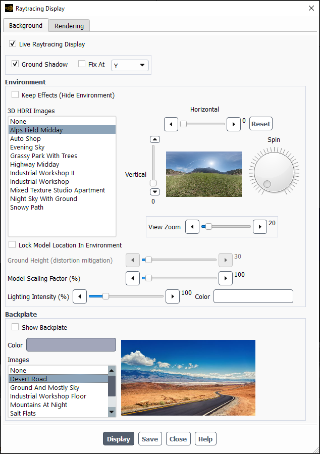
Controls
- Background
tab that contains settings for the environment and backplate, which can be used to provide lighting effects and a background to the displayed model. Changes made to settings on the Background tab while this option is enabled are automatically saved without the need to click .
- Live Raytracing Display
allows for changes made to controls in the Background tab to be immediately reflected in the raytracing window (which is only seen after you click ).
- Ground Shadow
displays shadows below the displayed object based on the lighting defined in the session as well as the lighting in the environment.
- Fix At
locks the plane location below the model so that the shadows are shown appropriately for the orientation of the displayed model. The axis that you specify should be the plane that is opposite to the pull of gravity. For example, if gravity is in the -Z direction, then select Z from the drop-down.
- Environment
group box containing options that control the environment that can be used to affect the appearance of the model.
- Keep Effects (Hide Environment)
this option keeps the effects of the environment on the model without showing the model in the environment. The background will be the same as the standard graphics display, unless you enable the Show Backplate option (in the Backplate group box).
- 3D HDRI Images
lists the available environments that you can use for your raytracing display. The light sources in these environments affect the appearance of the displayed model. A preview of each environment is shown in the image window to the right of the list.
- Vertical
slider that controls the orientation of the environment. Adjusting this slider moves the environment vertically.
- Horizontal
slider that controls the orientation of the environment. Adjusting this slider moves the environment horizontally.
resets the environment orientation.
- Spin
rotation control that controls the orientation of the environment. Adjusting the spin control rotates the environment either clockwise or counterclockwise.
- View Zoom
slider that controls the overall zoom level of the raytracing window (sometimes referred to as "field view"). Zooming in/out with this control changes the zoom level of the entire raytracing display window, including the environment and the model. You can then re-adjust the zoom level of the model by zooming in/out on the model in the original active window containing the interactive model display that is being raytraced.
- Lock Model Location In Environment
converts the environment from "limitless bounds" to "finite bounds", thus making it so that the displayed object always appears in the same location, even when rotated. Note that your raytracing display may require additional adjustment of the Ground Height to compensate for the distortion that can appear on vertical objects in the environment. The distortion comes because 3D HDRI images are spherical.
- Ground Height (distortion mitigation)
(only available when Lock Model Location in Environment is enabled) controls where the ground height appears in within the sphere that is the environment. Adjusting this slider can help address some of the distortion that may appear on vertical objects due to the rounded nature of the spherical environment.
- Model Scaling Factor
controls how large or small the displayed object appears in relationship to the environment.
- Lighting Intensity
slider controlling the intensity of the lighting for the selected environment. Moving the slider to the right increases the intensity of the light and moving it to the left decreases it.
- Color
specifies the color that will be used to color the environment lighting.
- Backplate
group box containing options that control the backplate that can be displayed behind the model.
- Show Backplate
controls whether or not a backplate is displayed behind the model in the raytracing window. When this option is enabled, the Color will be used unless you select an image from the Images list. The backplate will always be displayed "over top" of any selected environment.
- Color
specifies the color that will be displayed as the background behind the model when Show Backplate is enabled and Images is set to None.
- Images
lists the available 2D backplates that you can use for your raytracing display. The selected image will be displayed as the background behind the model when Show Backplate is enabled. A preview of each image is shown in the window to the right of the list.
- Rendering
tab that contains settings controlling how the raytracer functions and how pictures or hardcopies are saved.
- CPU Threads
specifies how many processors are used by the raytracer in rendering the image. If the number of CPU Threads specified is greater than the number of cores on the machine, the raytracer will use the maximum number available.
- Quality
specifies how "good" an image looks when rendered and saved as hardcopy picture. Better quality renderings are more expensive, that is they require more machine resources and take longer to render.
opens the Save Picture dialog box (Save Picture Dialog Box), allowing you to capture a hardcopy of the raytracer rendering.
specifies how long Fluent waits for the raytracer to render the display to the specified Quality before capturing the image.
saves the current settings and displays the raytracer rendering of the active graphics window according to the specified settings.
saves the raytracer settings. This allows you to define a raytracer rendering and save a picture without displaying it in the graphics window first.
The Reduced Order Model dialog box allows you to enable the reduced order model (ROM) and select which variables and zones to include in the ROM—refer to Creating Reduced Order Models (ROMs) additional information. You can also use it to evaluate a produced ROM as discussed in Reduced Order Model (ROM) Evaluation in Fluent.
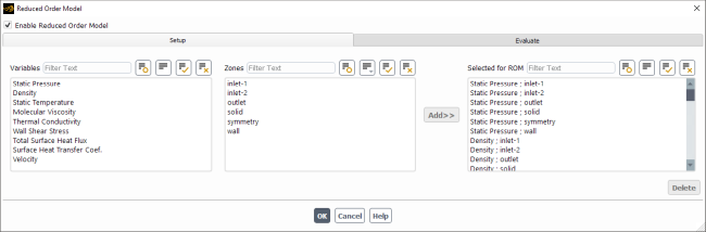
Controls
Setup tab
- Variables
lists the variables that are available for creating the ROM.
lists all of the zones in your case. You can select from this list to tell the ROM where the selected variables in the Variables list will be evaluated.
adds the selected variables and zones to the ROM.
- Selected for ROM
lists all of the selected variables and their associated locations for the ROM.
removes the selected variables and zones from the Selected for ROM list.
Evaluate tab
- Parameters used for ROM creation:
lists all of the variables that were used in creation of the reduced order model (ROM). The Min-Max Range on the right of the fields lists the accepted input ranges for the number entry fields.
- Evaluate
evaluates the case using the values you specify for the listed parameters.
The Reference Frame dialog box allows you to create local reference frames either with the coordinates and orientation that you specify or by tracking a cell zone. Refer to Reference Frames additional information.
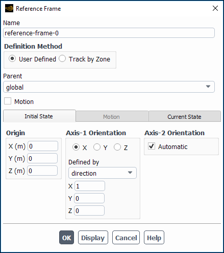
Controls
- Definition Method
specifies how you want to define the reference frame.
specifies the parent reference frame.
specifies which cell zone this reference frame will track.
- Motion (User Defined Only)
allows you to specify a motion for this reference frame (accomplished in the Motion tab.
- Linear Velocity (Motion tab)
is the linear velocity with respect to the parent reference frame orientation.
- Rotational Velocity (Motion tab)
is the rotational velocity with respect to the parent reference frame orientation.
- Rotation Axis
is the axis about which the rotational velocity will be applied.
- Origin
specifies the origin of the reference frame.
specifies the orientation of the selected axis.
- Axis-2 Orientation
specifies the orientation of the second axis. By default Fluent does this automatically, however you can disable Automatic and specify the orientation manually.
- Current State (tab)
shows you the current origin and axes directions of the reference frame with respect to the global reference frame.
The Replace Cell Zone dialog box allows you to replace a single cell zone or multiple zones. See Replacing Zones for details.
![]() Domain → Zones
→ Replace Zone...
Domain → Zones
→ Replace Zone...
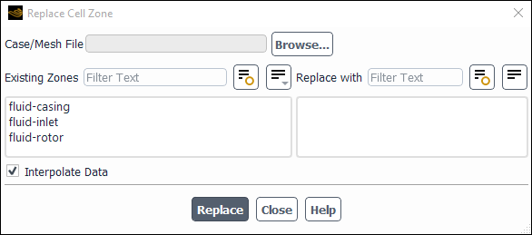
Controls
- Case/Mesh File
allows you to specify a mesh file from which you want to replace the zone.
- Existing Zones
contains a list of cell zones from which you can select the zone to be replaced.
- Replace with
contains a list of cell zones from which you can select the zone to replace the zone selected in Existing Zones list.
- Interpolate Data
allows you to enable/disable data interpolation if data already exists.
- Replace
replaces the selected cell zone.
![]() Solution → Reports
→ Definitions → Edit...
Solution → Reports
→ Definitions → Edit...
For information on creating report definitions, see Monitoring and Reporting Solution Data.
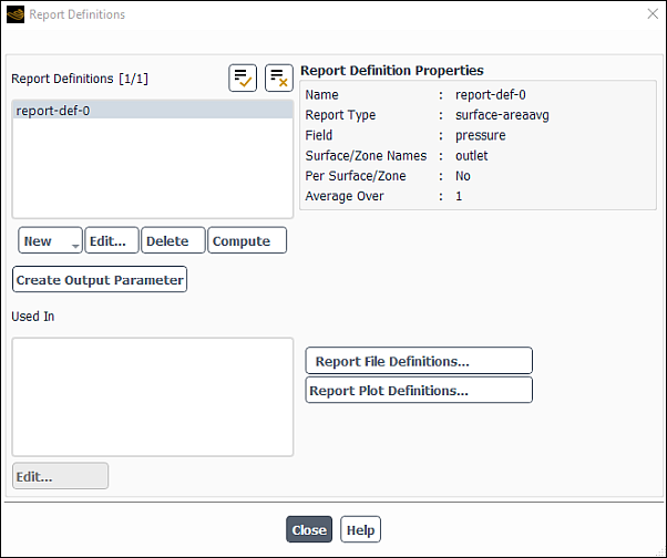
Controls
- Report Definitions
lists all of the existing report definitions.
- New
drop-down list allowing you to create new report definitions (surface, volume, force, flux, mesh, aeromechanics, dpm, expression, and user-defined).
- Edit...
allows you to edit the properties of the selected report definition.
- Delete
deletes the selected report definition.
- Compute
computes the value of the selected report definition and prints to the console.
- Create Output Parameter
creates an output parameter for the selected report definition(s) with the name
<report definition name>-op.- Used In
lists the report files and report plots that contain the selected report definition.
- Edit... (button)
opens the report file/plot dialog box for the report file/plot selected in the Used In list.
- Report Definition Properties
displays the properties of the selected report definition in the Report Definition list.
- Report File Definitions...
opens the Report File Definitions Dialog Box.
- Report Plot Definitions
opens the Report Plot Definitions Dialog Box.
![]() Solution → Reports
→ File...
Solution → Reports
→ File...
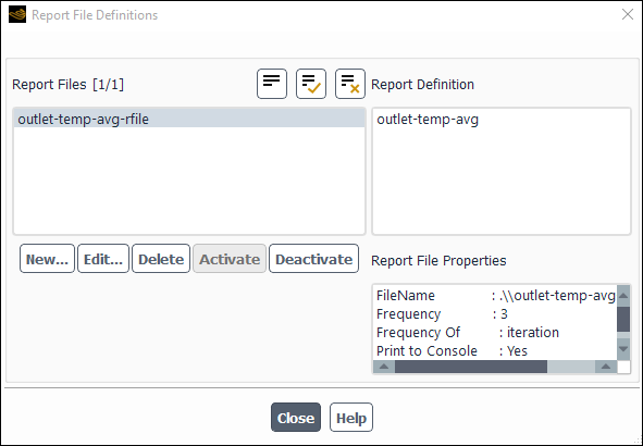
Controls
- Report Files
lists all of the existing report files.
- New...
opens the New Report File Dialog Box.
- Edit...
allows you to edit the properties of the selected report file in the Edit Report File Dialog Box.
- Delete
deletes the selected report file.
- Activate
activates the selected (previously deactivated) report file for writing during the solution calculation.
- Deactivate
deactivates the writing of the selected report file during the solution calculation.
- Report Definition
lists the report definitions included in the selected report file.
- Report File Properties
lists the properties of the selected report file.
![]() Solution → Reports
→ Plot...
Solution → Reports
→ Plot...
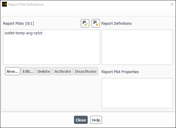
Controls
- Report Plots
lists all of the existing report plots.
- New...
opens the New Report Plot Dialog Box.
- Edit...
allows you to edit the properties of the selected report plot in the Edit Report Plot Dialog Box.
- Delete
deletes the selected report plot.
- Activate
activates the selected (previously deactivated) report plot for plotting during the solution calculation.
- Deactivate
deactivates the plotting of the selected report plot during the solution calculation.
- Report Definition
lists the report definitions included in the selected report plot.
- Report Plot Properties
lists the properties of the selected report plot.
You can use the Residual Monitors dialog box to control the residual information that Fluent reports. See Monitoring Residuals for details about the items below.
![]() Solution → Reports
→ Residuals...
Solution → Reports
→ Residuals...
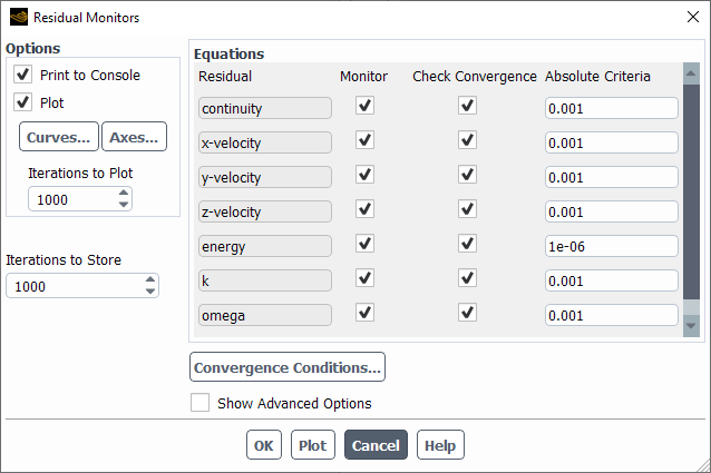
Controls
- Options
selects any combination of the following methods for reporting residuals. See Printing and Plotting Residuals for details.
- Print to Console
specifies whether or not to print residuals in the text window after each iteration.
- Plot
specifies whether or not to plot residuals in the graphics window after each iteration. See Plot Parameters for details.
- Iterations to Plot
is the number of history points to display on the residual plot.
- Axes...
opens the Axes Dialog Box, which allows you to modify the attributes of the axes.
- Curves...
opens the Curves Dialog Box, which allows you to modify the attributes of the residual curves.
- Iteration to Store
sets the number of residual history points to be stored in the data file. Due to the compaction algorithm used, saving 1000 points does not result in just the last 1000 iterations being saved; the history reaches back quite a bit further than that, but does not save a point at every iteration. Further back in the iteration history, the spacing between saved iterations grows larger. See Storing Residual History Points for details.
opens the Convergence Conditions Dialog Box.
- Residual
indicates the name of each variable for which residual information is available.
- Monitor
indicates whether or not the residuals for each variable are to be monitored. You can toggle monitoring on and off for each variable by turning the corresponding check box in the Monitor list on or off.
- Normalization Factor
shows the normalization factor for each variable. The default is the maximum residual value after the first 5 iterations. To set this value manually, enter a new value in the corresponding Normalization Factor field. This list will not appear if the Normalize option is turned off.
- Check Convergence
indicates whether or not the convergence of each variable is to be monitored. If convergence is being monitored, the solution will stop automatically when each variable meets its specified convergence criterion. You can check convergence only for variables for which you are monitoring residuals. You can toggle convergence checking on and off for each variable by turning the corresponding check box in the Check Convergence list on or off.
- Absolute Criteria, Relative Criteria
shows the residual value for which the solution of each variable will be considered to be converged. To set this value manually, enter a new value in the corresponding Absolute Criteria/Relative Criteria field.
- Plot
displays the current residual history plot.
Show Advanced Options
- Residual Values
controls the normalization and scaling of residuals. See Controlling Normalization and Scaling for details.
- Normalize
specifies whether or not to normalize the printed or plotted residual for each variable by the value indicated as the Normalization Factor for that variable. The default Normalization Factor is the maximum residual value after the first 5 iterations.
This option is off by default.
- Iterations
sets the number of iterations for which Ansys Fluent will search for the largest residual to normalize by. (If the Normalize option is turned off, this item will not be editable.)
- Scale
specifies whether or not to print or plot scaled residuals for each variable. This option is on by default.
- Compute Local Scale
computes and stores both the locally and globally scaled residuals from subsequent iterations, for the purpose of reporting. You will select the type of residual scaling form the Reporting Option drop-down list. See Definition of Residuals for the Pressure-Based Solver and Definition of Residuals for the Density-Based Solver for more information.
- Reporting Option
gives you the choice of plotting or printing to the console the global scaling or local scaling of residuals.
- Renormalize
sets the normalization factors to the maximum values in the residual histories. Renormalize should be used to renormalize the residual plot in cases where the maximum residuals occur sometime after the first five iterations.
- Convergence Criterion
consists of four options that are available for checking an equation for convergence.
- absolute
is the default and is available for steady-state cases. The residual (scaled and/or normalized) of an equation at an iteration is compared with a user-specified value. If the residual is less than the user-specified value, that equation is deemed to have converged for a time step.
- relative
is where the residual of an equation at an iteration of a time step is compared with the residual at the start of the time step. If the ratio of the two residuals is less than a user-specified value, that equation is deemed to have converged for a time step.
- relative or absolute
is where either the absolute convergence criterion or the relative convergence criterion is met. At that point, the equation is considered converged.
- none
is used to disable convergence checking.
The Rotate Mesh dialog box allows you to rotate the mesh about the required axis and rotation origin by specifying the angle of rotation. See Rotating the Mesh for details.
![]() Domain → Mesh
→ Transform → Rotate...
Domain → Mesh
→ Transform → Rotate...
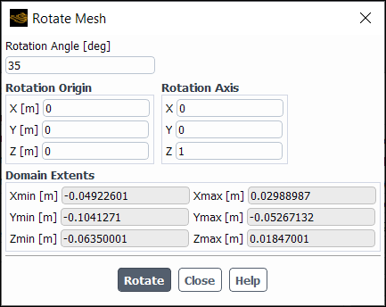
Controls
- Rotation Angle
is the angle with which you want to rotate the mesh. You can enter a positive or negative real number.
- Rotation Origin
defines the new origin for the mesh rotation.
- Rotation Axis
defines the axis about which you want to rotate the mesh.
- Domain Extents
displays the Cartesian coordinate extremes of the nodes in the mesh. (These values are not editable; they are purely informational.)
- Rotate
adds the specified rotation parameters to the appropriate Cartesian coordinate of every node in the mesh.
The S2S Information dialog box allows you to report values of the view factor and radiation emitted from one zone to any other zone. See Reporting Radiation in the S2S Model for details about the items below.
![]() Results → Model Specific
→ S2S Information...
Results → Model Specific
→ S2S Information...
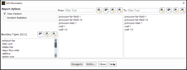
Controls
- Report Options
contains items for which information is available for reporting.
- View Factors
turns on the computation of view factors from one zone to the other.
- Incident Radiation
turns on the computation of the incident radiation from one zone to the other.
- Boundary Types
contains a selectable list of types of boundary zones. If you select (or deselect) an item in this list, all zones of that type will be selected (or deselected) automatically in the From and To lists.
- From
contains a selectable list of boundary zones for which you would like data reported from the selected zone.
- To
contains a selectable list of boundary zones for which you would like data reported to the selected zone.
computes the view factors and/or incident radiation on the selected zones.
opens The Select File Dialog Box, which you can use to save the data as an S2S Info File (
.sifformat).
The Select UDM Zones dialog box allows you allocate user-defined memory on specific zones. This dialog box is opened by clicking in the User-Defined Memory Dialog Box.
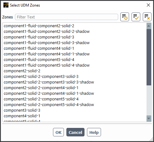
Controls
- Zones
lists the zones available for user-defined memory allocation.
confirms the selection of the highlighted zone(s) for user-defined memory allocation.
The Select Window dialog box allows you specify the window where the specified object (accessed via right-clicking the object or boundary in the tree and selecting Display in → More... or Add To → More...) will be displayed. See Managing Multiple Graphics Windows for additional information.
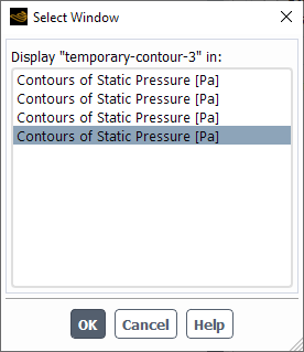
Controls
- Display <object/boundary name> in: | Add <object/boundary name> to:
lists the available graphics windows for display. Selecting a graphics window from the list makes the window active.
displays the specified object or boundary in the selected graphics window.
The Separate Cell Zones dialog box allows you to separate a single cell zone into multiple zones of the same type. See Separating Zones for details.
![]() Domain → Zones
→ Separate → Cells...
Domain → Zones
→ Separate → Cells...
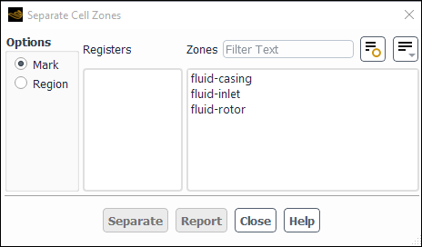
Controls
- Options
specifies the method on which the cell-zone separation is to be based.
- Mark
indicates that the cell zone is to be separated based on the marks stored in cell registers.
- Region
indicates that the cell zone is to be separated into two or more contiguous regions based on an internal boundary within the original zone.
- Registers
contains a list of defined cell registers. If you are separating the cell zone by mark, select the cell register to be used in the Registers list. When the separation is performed, cells that are marked will be placed into a new zone.
- Zones
contains a list of cell zones from which you can select the zone to be separated.
- Separate
separates the selected cell zone based on the specified parameters.
- Report
reports what the result of the separation will be without actually separating the cell zone.
The Separate Face Zones dialog box allows you to separate a single face zone into multiple zones of the same type. See Separating Zones for details.
![]() Domain → Zones
→ Separate → Faces...
Domain → Zones
→ Separate → Faces...
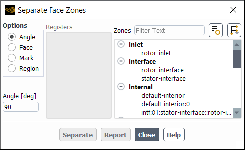
Controls
- Options
specifies the method on which the face zone separation is to be based.
- Angle
indicates that the face zone is to be separated based on significant angle (specified in the Angle field).
- Face
indicates that the face zone is to be separated by putting each face in the zone into its own zone.
- Mark
indicates that the face zone is to be separated based on the marks stored in cell registers.
- Region
indicates that the face zone is to be separated based on contiguous regions.
- Registers
contains a list of defined cell registers. If you are separating faces by mark, select the cell register to be used in the Registers list. When the separation is performed, all faces of cells that are marked will be placed into a new face zone.
- Zones
contains a list of face zones from which you can select the zone to be separated.
- Angle
specifies the significant angle to be used when you separate a face zone based on angle. Faces with normal vectors that differ by an angle greater than or equal to the specified significant angle will be placed in different zones when the separation occurs.
- Separate
separates the selected face zone based on the specified parameters.
- Report
reports what the result of the separation will be without actually separating the face zone.
The Set Injection Properties dialog box allows you to define the properties of an existing discrete-phase injection (which was created in the Injections Dialog Box). See Defining Injection Properties for details about the items listed in this section.
The Set Injection Properties dialog box is opened from the Injections Dialog Box.
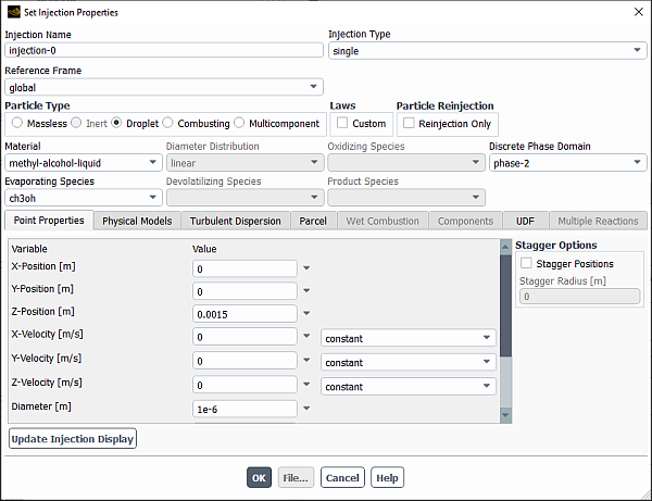
Controls
- Injection Name
sets the name of the injection.
- Injection Type
contains a drop-down list of the available injection types: single, group, cone, surface, volume, plain-orifice-atomizer, pressure-swirl-atomizer, air-blast-atomizer, flat-fan-atomizer, effervescent-atomizer, and file. (cone is not available in 2D.) These choices are described in Injection Types.
- Number of Streams
indicates the number of particle streams in a group, cone, or atomizer injections, or surface injections with the Randomize Starting Points option. (This item will not appear for single, volume, or file injections, or surface injections without the Randomize Starting Points option.)
- Reference Frame
is a drop-down list where you can select the reference frame for the injection point properties. By default, the global reference frame is used. This item is not available for surface, volume, and condensate injections.
- Injection Surfaces
is where you can select the surface(s) from which the particles in a surface injection will be released. This item will appear only for a surface injection.
- Release From
is where you can select either the zone or bounding-geometry particle release region. This item will appear only for a volume injection.
- Zones
is where you can select the zone(s) from which the particles in a volume injection will be released. This item will appear only when zone is selected from the Release From drop-down list.
- Bounding Shape
is a drop-down list where you can select sphere, cylinder, cone, or hexahedron to model the particle release region. This item will appear only when bounding-geometry is selected from the Release From drop-down list.
- Shape Coordinates
designates the coordinates to define the geometry of the selected bounding shape. See Defining Injection Properties for more information. This item will appear only when bounding-geometry is selected from the Release From drop-down list.
- Parcel Specification
specifies the number of particle parcels to be injected. You can choose either the number-of-starting-points or parcels-per-cell specification method. See Defining Injection Properties for details. This item appears only for a volume injection and is not available for DDPM cases with the Discrete Phase Domain setting other than none.
- Injection Packing Limit per Cell
specifies the highest particle volume fraction that is possible in a computational cell. See Defining Injection Properties for details. This item appears only for a volume injection when the DDPM with the Discrete Phase Domain setting other than none is used.
- Particle Type
specifies the particle type as Massless, Inert, Droplet, Combusting, or Multicomponent. These types are described in Particle Types.
- Laws
(not for massless particles) contains inputs for customized particle laws.
- Custom
enables the specification of customized particle laws and opens the Custom Laws Dialog Box.
- Reinjection Only
(unsteady particle tracking only) specifies whether the injection is used only for reinjecting particles as described in The reinject Boundary Condition.
- Material
(not for massless particles) indicates the material for the particles. If this is the first time you have created a particle of this type, you can choose from all of the materials by copying them from the database or creating them from scratch, as discussed in Setting Discrete-Phase Physical Properties and described in detail in Using the Create/Edit Materials Dialog Box.
- Diameter Distribution
(not for massless particles) allows you to select one of the following interpolation methods for determining the size of the particles:
linear (default, group injections only)
uniform (default, surface and volume injections only)
rosin-rammler
rosin-rammler-logarithmic
tabulated (cone, surface or volume injections only)
Selecting tabulated opens the Association of Particle Size Distribution Data dialog box.
See Using the Rosin-Rammler Diameter Distribution Method and Using the Tabulated (Discrete) Diameter Distribution for more information on the Rosin-Rammler method and the tabulated method, respectively.
- Evaporating Species
(for droplet particles) specifies the gas-phase species created by the vaporization and boiling laws (laws 2 and 3).
- Devolatilizing Species
(for combusting particles) specifies the gas-phase species created by the devolatilization law (law 4).
This item will not appear for two-mixture-fraction non-premixed combustion calculations.
- Devolatilizing Stream
(for combusting particles) specifies the destination stream for the gas-phase species created by the devolatilization law (law 4).
This item will appear only for two-mixture-fraction non-premixed combustion calculations.
- Oxidizing Species
(for combusting particles) specifies the gas phase species that participates in the surface char combustion reaction (law 5).
- Product Species
(for combusting particles) specifies the gas-phase species created by the surface char combustion reaction (law 5).
This item will not appear for two-mixture-fraction non-premixed combustion calculations.
- Product Stream
(for combusting particles) specifies the destination stream for the gas-phase species created by the surface char combustion reaction (law 5).
This item will appear only for two-mixture-fraction non-premixed combustion calculations.
- Discrete Phase Domain
is available when using the Dense Discrete Phase Model, described in Including the Dense Discrete Phase Model.
- DEM Collision Partner
is available when using the DEM Collision model, described in Modeling Collision Using the DEM Model.
- Point Properties
displays the inputs for the point properties for the injection (for example, position, velocity, diameter, temperature, mass flow rate, and stagger options). These inputs are described for each injection type in Point Properties for Single Injections – Point Properties for Effervescent Atomizer Injections.
- Stagger Options
allows you to set the stagger options:
- Stagger Positions
enables injection-specific spatial staggering of the particles.
- Stagger Radius
specifies the region from which particles are released. This item is available only for non-atomizer injections.
- Stagger in Injection Plane Only
when enabled, restricts the spatial staggering of the initial particle positions to purely the radial direction of the spray. The spatial staggering clusters the initial particle positions about the outer radius of the hollow cone using a Gaussian distribution with 0 mean and +/- 2 standard deviation. This item is available only for hollow-cone injections.
- Surface Options
(surface injections only) allows you to select the following options:
- Scale Flow Rate by Face Area
scales the individual mass flow rates of the particles by the ratio of the area of the face they are released from to the total area of the surface.
- Inject Using Face Normal Direction
uses the surface normal for the injection direction. When this option is selected, you need to specify only the velocity magnitude of the injection, not the individual components of the velocity magnitude.
- Randomize Starting Points
when this option is selected, particles are injected from positions distributed randomly over the selected boundary surfaces.
- Wallfilm
(surface injections only) is where you can select the Inject Wallfilm Particles option if you want to inject wall film particles from surfaces. This item is available for unsteady particle tracking only.
- First Point
specifies the first point properties for the injection. This item appears only for group injections.
- Last Point
specifies the last point properties for the injection. This item appears only for group injections.
- Update Injection Display
applies the current point property settings to the injection graphics windows so that you can preview the effect of modified settings before saving the injection. This item is not available for surface, volume, file, and condensate injection types.
- Use Mass Instead of Flow Rate
When selected, you can specify the Total Mass instead of the default Total Flow Rate of the parcel to be injected into the particle release region. This item is available only for the volume injection type.
- Physical Models
displays the inputs for injection-specific physics models.
- Drag Parameters
allows the setting of the drag law used in calculating the force balance on the particles. See Particle Force Balance in the Theory Guide for details on the items below.
- Drag Law
is a drop-down list containing the available choices for the drag law:
- spherical
assumes that the particles are smooth spheres.
- nonspherical
assumes that the particles are not spheres, but are all identically shaped. The shape is specified by the Shape Factor.
- Stokes-Cunningham
is for use with sub-micron particles. A Cunningham Correction is added to Stokes’ drag law to determine the drag.
- high-Mach-number
is similar to the spherical law with corrections to account for a particle Mach number greater than 0.4 or a particle Reynolds number greater than 20.
- Ishii-Zuber
is used in gas-liquid flows. This drag law is only available if the magnitude and direction of the gravity vector are specified in the Operating Conditions dialog box. See Ishii-Zuber Drag Model in the Fluent Theory Guide for details.
- Grace
is used in gas-liquid flows. This drag law is only available if the magnitude and direction of the gravity vector are specified in the Operating Conditions dialog box. See Grace Drag Model in the Fluent Theory Guide for details.
- dynamic-drag
accounts for the effects of droplet distortion. This drag law is available only when one of the droplet breakup models is used in conjunction with unsteady tracking. See Dynamic Drag Model Theory in the Theory Guide for details.
- Shape Factor
specifies the shape of the particles when nonspherical is selected as the Drag Law (
 in Equation 12–52 in the Theory Guide). It is
the ratio of the surface area of a sphere having the same volume as
the particle to the actual surface area of the particle. The shape
factor value cannot be greater than
in Equation 12–52 in the Theory Guide). It is
the ratio of the surface area of a sphere having the same volume as
the particle to the actual surface area of the particle. The shape
factor value cannot be greater than 1.- Cunningham Correction
(
 in Equation 12–55 in the Theory Guide) is used
with Stokes’ drag law to determine the force acting on the particles
when the particles are sub-micron size. It appears when Stokes-Cunningham is selected as the Drag Law.
in Equation 12–55 in the Theory Guide) is used
with Stokes’ drag law to determine the force acting on the particles
when the particles are sub-micron size. It appears when Stokes-Cunningham is selected as the Drag Law.- Wen-Yu
uses the fluid-solid drag function of Wen and Yu described in Fluid-Solid Exchange Coefficient in the Fluent Theory Guide. See Specifying the Drag Function for recommendations on the usage of this option. This drag law is available only when the dense discrete phase model (DDPM) is enabled.
- Gidaspow
uses the Gidaspow formulation described in Fluid-Solid Exchange Coefficient in the Fluent Theory Guide. See Specifying the Drag Function for recommendations on the usage of this drag law. This drag law is available only when the dense discrete phase model (DDPM) is enabled.
- Huilin-Gidaspow
uses the Huilin-Gidaspow function described in Fluid-Solid Exchange Coefficient in the Fluent Theory Guide. See Specifying the Drag Function for recommendations on the usage of this drag law. This drag law is available only when the dense discrete phase model (DDPM) is enabled.
- Syamlal-OBrien
uses the Syamlal-O’Brien model described in Fluid-Solid Exchange Coefficient in the Fluent Theory Guide. See Specifying the Drag Function for recommendations on the usage of this drag law. This drag law is available only when the dense discrete phase model (DDPM) is enabled.
- Gibilaro
uses the Gibilaro model described in Fluid-Solid Exchange Coefficient in the Fluent Theory Guide. See Specifying the Drag Function for recommendations on the usage of this drag law. This drag law is available only when the dense discrete phase model (DDPM) is enabled.
- EMMS
uses the energy-minimization multi-scale (EMMS) drag model described in Fluid-Solid Exchange Coefficient in the Fluent Theory Guide. See Specifying the Drag Function for recommendations on the usage of this drag law. This drag law is available only when the dense discrete phase model (DDPM) is enabled.
- Filtered
uses the filtered Two-Fluid Model (TFM) described in The Filtered Two-Fluid Model in the Fluent Theory Guide. See Specifying the Drag Function for recommendations on the usage of this drag law. This drag law is available only when the dense discrete phase model (DDPM) is enabled.
- Heat Transfer Coefficient
is a drop-down list from which you can select the heat transfer model for your simulation. See Heat Transfer Coefficient for a full description of available models and their usage.
- Particle Rotation
contains settings for the modeling of particle rotation when the Enable Rotation check box is selected (see Wall-Particle Reflection Model Theory in the Fluent Theory Guide).
- Rotational Drag Law
is a drop-down list of available rotational drag law models:
- Dennis-et-al
uses Equation 12–67 in the Fluent Theory Guide to calculate the rotational drag coefficient
 .
.- none
implies zero torque, that is, it excludes the influence of the fluid on the rotational particle motion.
- Magnus Lift Law
is a drop-down list of available Magnus lift law models:
- Oesterle-Bui-Dinh
uses Oesterle and Bui Dinh’s formulation (Equation 12–18 in the Fluent Theory Guide).
- Tsuji-et-al
is based on the particle spin rate (Equation 12–19 in the Fluent Theory Guide).
- Rubinow-Keller
uses a linear dependence of the rotational lift coefficient
 on the spin
rate (Equation 12–21 in the Fluent Theory Guide).
on the spin
rate (Equation 12–21 in the Fluent Theory Guide).- none
implies that the Magnus lift will not be included in your simulation.
- Brownian Motion
enables the incorporation of the effects of Brownian motion. This option is available only when the Energy equation is enabled (in the Models group) and the Stokes-Cunningham drag law is selected from the Drag Law drop-down list. See Brownian Force in the Theory Guide for details.
- Breakup
contains parameters that control droplet breakup and collision. (This section of the dialog box appears only if Unsteady Tracking is enabled in the Discrete Phase Model Dialog Box.) See Breakup for more information.
- Enable Breakup
enables breakup for this injection.
- Breakup Model
is a drop-down list containing parameters that control droplet breakup. (This item appears only if Enable Breakup is selected.)
- TAB
enables the Taylor Analogy Breakup (TAB) model, which is applicable to many engineering sprays. This method is based upon Taylor’s analogy between an oscillating and distorting droplet and a spring mass system. See Taylor Analogy Breakup (TAB) Model in the Theory Guide for details.
For the TAB model, you must specify the following constants:
- y0
is the constant
 in Equation 12–408 in the Theory
Guide.
in Equation 12–408 in the Theory
Guide.- Breakup Parcels
is the number of child parcels the droplet is split into, as described in Velocity of Child Droplets in the Theory Guide.
- Wave
enables the Wave breakup model, which considers the breakup of the injected liquid to be induced by the relative velocity between the gas and liquid phases. See Wave Breakup Model for details.
For the Wave model, you must specify the following constants:
- B0
is the constant
 in Equation 12–435 in the Theory
Guide.
in Equation 12–435 in the Theory
Guide.- B1
is the constant
 in Equation 12–437 in the Theory
Guide.
in Equation 12–437 in the Theory
Guide.
- KHRT
enables the Kelvin-Helmholtz Rayleigh-Taylor breakup model, which considers the two competing effects of aerodynamic breakup and instabilities due to droplet acceleration. See KHRT Breakup Model in the Theory Guide for details.
For the KHRT model, you must specify the following constants:
- B0
is the constant
in Equation 12–435 in the Theory
Guide.- B1
is the constant
in Equation 12–437 in the Theory
Guide.- Ctau
is the constant
 in Equation 12–442 in the Theory
Guide.
in Equation 12–442 in the Theory
Guide.- CRT
is the constant
 in Equation 12–443 in the Theory
Guide.
in Equation 12–443 in the Theory
Guide.- CL
is the constant
 in Equation 12–438 in the Theory
Guide.
in Equation 12–438 in the Theory
Guide.
- SSD
enables the stochastic secondary droplet breakup model, where the probability of breakup is independent of the parent droplet size and the secondary droplet size is sampled from an analytical solution of the Fokker-Planck equation for the probability distribution. See Stochastic Secondary Droplet (SSD) Model in the Theory Guide for details.
For the SSD model, you must specify the following constants:
- Critical We
is the critical Weber number in Equation 12–444 in the Theory Guide.
- Core B1
is B in Equation 12–445 in the Theory Guide.
- Target Np
is the average number in parcels for daughter parcels.
- Xi
is
 in Equation 12–446 in the Theory Guide.
- Madabhushi
Enables the Madabhushi breakup model. This model is available only with single, group, or cone (solid cone) injections. Solid cone injection is recommended. For more information about the Madabhushi breakup model, see Madabhushi Breakup Model in the Fluent Theory Guide.
For the Madabhushi model, you must specify the following constants:
- B0
is the constant
in Equation 12–435 in the Theory
Guide. The recommended value is 2.44.- B1
is the constant
in Equation 12–437 in the Theory
Guide. The recommended value is 10.- Jet Diameter
is the nozzle orifice exit diameter.
- Ligament Factor
Adjusts the diameter of the child droplets arising from the column breakup mechanism
- C0
is the column breakup time constant. The value recommended for the Madabhushi breakup model is 3.44.
- Column Drag Cd
is the constant drag coefficient for calculating the drag force acting on droplets within the liquid column.
- Breakup Max Generation
is the maximum number of child parcel generations.
- Subsequent Statistical Breakup
when enabled, the droplet breakup mechanism switches to the subsequent statistical breakup model after the Breakup Max Generation is reached. No child parcels are created during the breakup mechanism. Instead, the particle number in the parcel is increased, and the particle diameter is adjusted in such a way as to conserve the full filling mass of the parent parcel.
- Schmehl
Enables the Schmehl breakup model. For more information about the Schmehl breakup model, see Schmehl Breakup Model in the Fluent Theory Guide.
For this model, you can specify the following settings:
- Breakup Parcels
is the number of child parcels generated after splitting the droplet as described in Schmehl Breakup Model in the Fluent Theory Guide.
- Breakup Max Generation
is the maximum number of child parcel generations.
- Subsequent Statistical Breakup
when enabled, the droplet breakup mechanism switches to the subsequent statistical breakup model after the Breakup Max Generation is reached.
- Turbulent Dispersion
displays the inputs for stochastic tracking.
- Stochastic Tracking
controls the stochastic tracking for turbulent flows. Stochastic tracking includes the effect of turbulent velocity fluctuations on the particle trajectories using the DRW model described in Stochastic Tracking in the Theory Guide. See Stochastic Tracking for details about the items below.
- Discrete Random Walk Model
includes the effect of instantaneous turbulent velocity formulations on the particle trajectories through stochastic method.
- Random Eddy Lifetime
specifies that the characteristic lifetime of the eddy is to be random.
- Number of Tries
controls the inclusion of turbulent velocity fluctuations.
An input of 1 or greater tells Ansys Fluent to include turbulent velocity fluctuations in the particle force balance.
- Time Scale Constant
is
 in Equation 12–24 in the Theory Guide. The default
is 0.15; if you use the RSM, a value of 0.3 is recommended.
in Equation 12–24 in the Theory Guide. The default
is 0.15; if you use the RSM, a value of 0.3 is recommended.
- Parcel
displays the inputs for controlling the discrete phase parcels. This tab is not available for volume injections when the DDPM with the Discrete Phase Domain option is used.
- Parcel Definitions
contains settings for how parcels are defined
- Parcel Release Method
specifies the method for releasing parcels. Available settings are standard, constant-number, constant-mass, and constant-diameter. See Steady/Transient Treatment of Particles for details about these settings.
- Wet Combustion
displays the inputs for the wet combustion model.
- Wet Combustion Model
allows the combusting particles to include an evaporating/boiling material.
- Liquid Material
contains a drop-down list of liquid materials that can be chosen as the evaporating/boiling material to be included with the combusting particles.
- Liquid Fraction
sets the volume fraction of the liquid present in the particle.
- Components
contains the inputs for the Multicomponent particle type. For details on the following items, see Defining Injection Properties. This item is available only when Multicomponent is selected as Particle Type.
- Multicomponent Settings
contains the multicomponent injections.
- Component
specifies the component that is a part of the multicomponent species.
- Mass Fraction
specifies the mass fraction of the component in a multicomponent species.
- Evaporating Species
specifies the gas-phase species to be evaporated.
- Evaporating Stream
specifies the source stream from which the species will be evaporated. This item appears only when the non/partially-premixed model is used in the case setup.
- UDF
displays the inputs for User-Defined Functions for use in the definition of the particle injection. For details about user-defined functions, see the separate Fluent Customization Manual.
- Initialization
contains a drop-down list of available user-defined functions. The UDF that you choose will be used to modify the injection properties at the time the particles are injected into the domain.
- Heat/Mass Transfer
allows you to select the user-defined function that defines the heat or mass transfer.
- Multiple Reactions
displays the inputs for Multiple Surface Reactions. See Combusting Particle Surface Reactions for details about this model.
- Species Mass Fractions
specify the combustible fraction of the combusting particle if you have defined more than one particle surface species. See Using the Multiple Surface Reactions Model for Discrete-Phase Particle Combustion for details.
- File...
opens The Select File Dialog Box, in which you can select a file containing the injection definition (when file is selected as the Injection Type).
The Set Multiple Injection Properties dialog box allows you to set properties that are common to multiple injections. See Defining Properties Common to More than One Injection for details about the items below.
The Set Multiple Injection Properties dialog box is opened from the Injections Dialog Box.
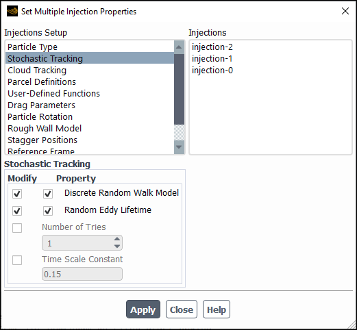
Controls
- Injections Setup
contains a list of the categories of injection properties that you can set for the injections in the Injections list. These categories correspond to the categories of inputs in the Set Injection Properties Dialog Box. When you select an item in the Injections Setup list, the dialog box will expand to show the relevant inputs, which are the same as those in the Set Injection Properties dialog box.
- Injections
displays an informational list of the injections for which you are setting common properties. These are the injections that you selected in the Injections Dialog Box.
The Sponge Layer dialog box creates or edits a sponge layer definition, which can be used to eliminate non-physical pressure wave reflections from boundary zones in transient simulations of compressible flows with the pressure-based solver, by blending the density from the value calculated by the solver to a user-specified far-field value in the domain near one or more specified boundary zones. It is opened by clicking or by making a selection from the Sponge Layers list and clicking in the Manage Sponge Layers Dialog Box. For further details, see Sponge Layers.
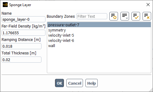
Controls
- Name
specifies the name of the sponge layer definition.
- Far-Field Density
specifies a value of density that is used for blending with the solver value within the sponge layer. It is recommended that you use the average density at the boundaries throughout the simulation.
- Ramping Distance
specifies a distance within the sponge layer over which the density changes from the solver value to the far-field value. It is recommended that this distance is 80–100% of the Total Thickness.
- Total Thickness
specifies the total thickness of the sponge layer, a distance from the selected boundaries to the interior boundary of the sponge layer. It is recommended that this thickness is at least twice the wavelength of the expected pressure waves.
- Boundary Zones
contains a list of available boundary zones on which the sponge layer can be applied.
The Structural Point Surface dialog box allows you to interactively create structural point surfaces (surfaces containing a single data point). See Structural Point Surfaces for details about the items below.
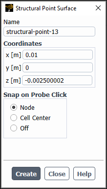
Controls
- Name
designates the name of the new surface. The default is the concatenation of the surface type and an integer which is the new surface ID.
- Reference Frame
allows you to specify a local reference frame (if defined) for the point surface.
- Coordinates
designates the coordinates of the point in the surface (x0, y0, z0).
- Snap on Probe Click
updates the coordinates of the point to the closest Node or Cell Center when you click on the model in the graphics window using the probe tool—that is, either by right-clicking or setting the left-mouse-button to probe (
).You can disable automatic snapping by selecting Off.
- Create
creates the surface.
The Surface Meshes dialog box allows you to read the surface meshes in Ansys Fluent (See Reading Surface Mesh Files for details on reading surface meshes.)
The Surface Meshes dialog box is opened from the Geometry Based Adaption Dialog Box.
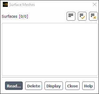
Controls
- Surfaces
contains a list of the surfaces available in the surface mesh you read.
You can select/deselect the surfaces listed under Surfaces.
- Read...
opens the Select File dialog box in which you can select the surface mesh you want to read.
- Delete
allows you to delete the selected surfaces under Surfaces area.
- Display
allows you to display the selected surfaces under Surfaces.
The Surface Rendering Properties dialog box is opened by clicking when By Surface is selected for Coloring in the Mesh Display Dialog Box.
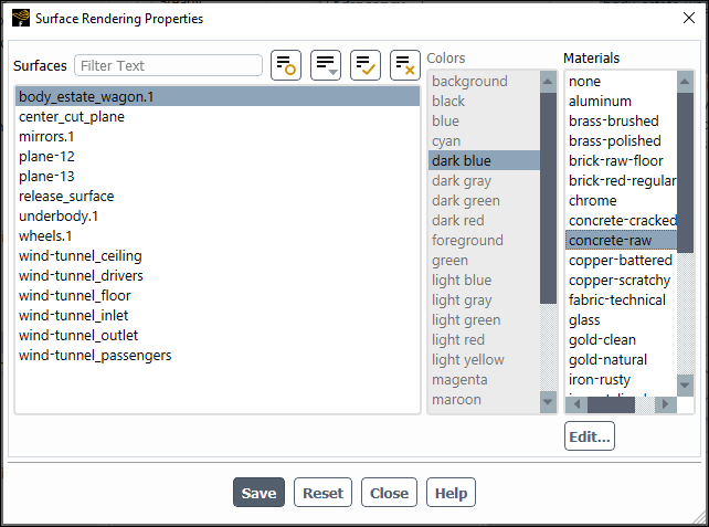
Controls
- Surfaces
contains a list of the surfaces where you can specify a color and/or material for rendering purposes.
- Colors
contains a list of the colors that you can apply to the surfaces selected in the Surfaces list.
- Materials
lists the available materials that may be used to color the surfaces selected in the Surfaces list. Click if you want to modify a material's color or other properties. See Creating Custom Realistic Materials for additional information.
opens the Material Editor Dialog Box.
Saves all specified surface and color/material assignments.
Resets all color and/or material assignments back to the default colors.
![]() Solution → Reports
→ Definitions → New
→ Surface Report
Solution → Reports
→ Definitions → New
→ Surface Report
Controls
- Name
specifies the name of the report definition.
- Options
- Per Surface
specifies whether or not the chosen field variable is calculated from all of the selected surfaces combined (default) or individually on each of the selected surfaces.
- Average Over
(optional) To have Fluent calculate a running average for the Surface Report Definition you can enter a positive integer greater than 1 (the default) for Average Over.
Specifying a number greater than 1 means that Fluent will print, plot, and write the running average value of the selected variable instead of the current value of the same variable.
The value reported is averaged over the last
iterations/time steps, where is your specified Average Over value.
When the iteration/time step number is lower than , Fluent calculates the average of the available variable
values.
- Retain Instantaneous Values
appears when Average Over is set to a value greater than
1. If enabled when you are creating a new report definition, it ensures that all instantaneous values are saved in the new report file that is being created for this report definition. It also results in the Plot Instantaneous Values option being enabled in the newly created report plot.
- Report Files
lists all of the report files where you can write the report definition data.
- Report Plots
lists all of the report plots where you can plot the report definition data (assuming this report has the same units as the other report definitions included in the selected report plot).
- Create
- Report File
creates a new report file that includes this report definition.
- Report Plot
creates a new report plot that includes this report definition.
- Frequency
specifies how frequently the report definition is written, plotted, or printed to the console.
- Print to Console
prints the value of the report definition to the console.
- Create Output Parameter
creates an output parameter for this report definition with the name
<report definition name>-op.- Report Type
selects the integration method used on the selected surfaces. The available report types are the same as those in the Surface Integrals Dialog Box. See Surface Integration for details.
- Custom Vectors
allows you to specify a vector if you selected Custom Vector Based Flux, Custom Vector Flux or Custom Vector Weighted Average from the Report Type drop-down list.
- Field Variable
contains a list of solution variables that can be monitored on the selected surfaces. This list will not be available if you select Mass Flow Rate or Volume Flow Rate as the Report Type.
- Phase
contains a list of all of the phases in the problem that you have defined. This is available when the VOF, mixture, or Eulerian multiphase model is enabled.
- Surfaces
contains a selectable list of the current surfaces.
- New Surface
is a drop-down list button that contains a list of surface options:
- Point
opens the Point Surface Dialog Box.
- Line/Rake
opens the Line/Rake Surface Dialog Box.
- Plane
opens the Plane Surface Dialog Box.
- Quadric
opens the Quadric Surface Dialog Box.
- Iso-Surface
opens the Iso-Surface Dialog Box.
- Iso-Clip
opens the Iso-Clip Dialog Box.
- Structural Point
opens the Structural Point Surface Dialog Box.
- OK
creates the report definition.
- Compute
computes the value of the report definition at the selected surface(s) and prints to the console.
The Surfaces dialog box allows you to interactively group, rename, and delete surfaces and obtain information about their components. See Grouping, Prioritizing, Editing, Renaming, and Deleting Surfaces for details about the items below.
Controls
- Surfaces
contains a list of existing surfaces from which you can select the surface(s) of interest.
- Name
displays the name of the selected surface. You can edit the text field to modify the surface name. (If more than one surface is selected, the name of the first one you selected will be displayed.)
- Surface Type
displays the type of surface that is selected (for example,
zone-surfif one surface is selected, orMultiple Surfacesif more than one surface is selected).- Points, 0D Facets, 1D Facets,
and 2D Facets display the number of points and facets in the selected surface. If more than one surface is selected, the sum over all selected surfaces is displayed for each quantity.
Note that if you want to check these statistics for a surface that was read from a case file, you will need to first display it.
- Rendering Priority
specifies the rendering priority for the selected surface, which determines which surface will be seen when there are coincident surfaces within a display.
- ID
displays the ID of the selected surface. You cannot change this value.
- UnGroup
ungroups the selected surface. This button is available only if the selected surface was created by Grouping two or more surfaces together.
- Rename
renames the selected surface in Surfaces with the name specified in Name. This button is available when just one surface is selected. (If two or more surfaces are selected, it becomes the Group button.)
- Group
groups two or more selected surfaces and gives the group the name entered in Name. This button replaces the Rename button when two or more surfaces are selected.
- Delete
deletes the selected surface(s).
The Thread Control dialog box allows you to control the maximum number of threads on each machine, as described in Controlling the Threads.
![]() Parallel → General → Thread Control...
Parallel → General → Thread Control...
Controls
- Maximum Number of Spawned Threads
contains a list of options for defining the maximum number of threads on each machine.
- Number of Node Processes on Machine
specifies that the maximum number of threads on each machine is equal to the number of Ansys Fluent node processes on each machine.
- Number of Cores on Machine
specifies that the maximum number of threads on each machine is equal to the number of cores on the machine. Ansys Fluent obtains the number of cores from the OS.
- Fixed Number
specifies that the maximum number of threads that can be spawned on each machine is equal to the number you provide in the number-entry box below Fixed Number.
The Time Averaged Explicit Thermal Coupling dialog box specifies transient conjugate heat transfer. Each coupling cycle is specified for a number of time steps at which the exchange of thermal boundary condition quantities occurs. See Time Averaged Explicit Thermal Coupling for details about the items below.
Controls
- Coupled Walls
list of coupled walls available for CHT.
- Selected for Time-Averaged Coupling
list of walls selected for CHT.
- Coupling Controls
contains options for the thermal coupling.
- Number of time steps per coupling iteration
specifies the number of time steps between coupling iterations.
- Moving Average
enables a moving average for the explicit coupling.
- Average Over
specifies the number of times steps over which the data is averaged for explicit coupling.
The Transform Surface dialog box allows you to create a new data surface by rotating and/or translating an existing surface, and/or by specifying a constant normal distance from it. See Transforming Surfaces for details about the items below.
![]() Domain → Surface
→ Create → Transform...
Domain → Surface
→ Create → Transform...
Controls
- Rotate
contains the transformation parameters for rotation.
- About
defines the origin about which the surface is rotated. You will specify a point, and the origin of the coordinate system for the rotation will be set to the specified point. For example, if you specified the point (1,0) in 2D, rotation would be about the
 axis anchored at (1,0). You can
either enter the point’s coordinates in the x,y,z fields or click the button and
select a point in the graphics window using the mouse.
axis anchored at (1,0). You can
either enter the point’s coordinates in the x,y,z fields or click the button and
select a point in the graphics window using the mouse.- Angles
define the angles about the x, y, and z axes (that is, the axes of the coordinate system with the origin defined under About) by which the surface is rotated. For 2D problems, you can specify rotation about the z axis only.
- Translate
contains the transformation parameters for translation.
- x,y,z
define the distance by which the surface is translated in each direction.
- Iso-Distance
contains the transformation parameters for “isodistancing.”
- d
sets the normal distance between the original surface and the transformed surface.
- Transform Surface
contains a list of existing surfaces from which you can select the surface to be transformed. The selected surface will remain unchanged; the transformation will create a new surface.
- New Surface Name
designates the name of the new surface. The default is the concatenation of the transformation type (that is, iso-distance, rotate, or translate) and an integer which is the new surface ID.
- Create
creates the surface.
The Translate Mesh dialog box allows you to change the origin of the mesh. See Translating the Mesh for details.
![]() Domain → Mesh →
Transform → Translate...
Domain → Mesh →
Transform → Translate...
Controls
- Translation Offsets
contains the desired changes in the mesh coordinates (that is, the desired delta in the axes origin). You can enter a positive or negative real number.
- X,Y,Z
defines the deltas in the
 ,
,  , and
, and  directions, in the current units of length.
- Domain Extents
displays the Cartesian coordinate extremes of the nodes in the mesh. (These values are not editable; they are purely informational.)
- Xmin, Ymin, Zmin
shows the minimum values of Cartesian coordinates in the mesh.
- Xmax, Ymax, Zmax
shows the maximum values of Cartesian coordinates in the mesh.
- Translate
adds the specified translation offsets to the appropriate Cartesian coordinate of every node in the mesh.
The Turbo 2D Contours dialog box enables you to display turbomachinery-specific contours of variables on surfaces of constant pitchwise, spanwise, or meridional coordinates, projected onto a plane. See Displaying Turbomachinery 2D Contours for details.
![]() Results → Model Specific
→ Turbo Topology → 2D
Contours...
Results → Model Specific
→ Turbo Topology → 2D
Contours...
Controls
- Turbo Topology
contains a list of defined topologies. Select from the list to display the values for the selected topology.
- Options
contains the check buttons that set various contour display options.
- Filled
toggles between filled contours and line contours.
- Node Values
toggles between using scalar field values at nodes and at cell centers for computing the contours.
- Global Range
toggles between basing the minimum and maximum values on the range of values on the selected surfaces (off), and basing them on the range of values in the entire domain (on, the default).
- Auto Range
toggles between automatic and manual setting of the contour range. Any time you change the Contours of selection, Auto Range is reset to on.
- Clip to Range
determines whether or not values outside the prescribed Min/ Max range are contoured when using Filled contours. If selected, values outside the range will not be contoured. If not selected, values below the Min value will be colored with the lowest color on the color scale, and values above the Max value will be colored with the highest color on the color scale. See Specifying the Range of Magnitudes Displayed for details.
- Levels
sets the number of contour levels that are displayed.
- Setup
indicates the ID number of the contour setup. For frequently used combinations of contour fields and options, you can store the information needed to generate the contour plot by specifying a Setup number and setting up the desired information in the dialog box. See Storing Contour Plot Settings for details.
- Contours of
contains a list from which you can select the scalar field to be contoured.
- Min
shows the minimum value of the scalar field. If Auto Range is off, you can set the minimum by typing a new value.
- Max
shows the maximum value of the scalar field. If Auto Range is off, you can set the maximum by typing a new value.
- Normalised Spanwise Coordinates (0 to 1)
enables you to specify the coordinate for the spanwise surface you want to create.
- Display
displays the contours in the active graphics window.
- Compute
calculates the scalar field and updates the Min and Max values (even when Auto Range is off).
The Turbo Averaged Contours dialog box
enables you to display turbomachinery-specific circumferentially averaged
contours of variables projected on an  -
-  plane. See Displaying Turbomachinery Averaged Contours for details.
![]() Results → Model Specific
→ Turbo Topology → Averaged
Contours...
Results → Model Specific
→ Turbo Topology → Averaged
Contours...
Controls
- Turbo Topology
contains a list of defined topologies. Select from the list to display the values for the selected topology.
- Options
contains the check buttons that set various contour display options.
- Filled
toggles between filled contours and line contours.
- Auto Range
toggles between automatic and manual setting of the contour range. Any time you change the Contours of selection, Auto Range is reset to on.
- Clip to Range
determines whether or not values outside the prescribed Min/ Max range are contoured when using Filled contours. If selected, values outside the range will not be contoured. If not selected, values below the Min value will be colored with the lowest color on the color scale, and values above the Max value will be colored with the highest color on the color scale. See Specifying the Range of Magnitudes Displayed for details.
- Levels
sets the number of contour levels that are displayed.
- Setup
indicates the ID number of the contour setup. For frequently used combinations of contour fields and options, you can store the information needed to generate the contour plot by specifying a Setup number and setting up the desired information in the dialog box. See Storing Contour Plot Settings for details.
- Contours of
contains a list from which you can select the scalar field to be contoured.
- Min
shows the minimum value of the scalar field. If Auto Range is off, you can set the minimum by typing a new value.
- Max
shows the maximum value of the scalar field. If Auto Range is off, you can set the maximum by typing a new value.
- Domain Min
shows the global minimum value of the scalar field for the entire domain.
- Domain Max
shows the global maximum value of the scalar field for the entire domain.
- Display
displays the contours in the active graphics window.
- Compute
calculates the scalar field and updates the Min and Max values (even when Auto Range is off).
The Turbo Averaged XY Plot dialog box enables you to display data in an XY plot format as a function of either the meridional or the spanwise coordinate. See Generating Averaged XY Plots of Turbomachinery Solution Data for details.
![]() Results → Model Specific
→ Turbo Topology → Averaged XY
Plot...
Results → Model Specific
→ Turbo Topology → Averaged XY
Plot...
Controls
- Y Axis Function
contains a list of solution variables that can be used for the
 axis of the plot.
- Min
shows the minimum value of the scalar field.
- Max
shows the maximum value of the scalar field.
- Turbo Topology
contains a list of defined topologies. Select from the list to display the values for the selected topology.
- X Axis Function
enables you to select the coordinate to be used for the
 axis of the plot. The choices are Hub
to Casing Distance (spanwise coordinate), and Meridional Distance (meridional coordinate).
axis of the plot. The choices are Hub
to Casing Distance (spanwise coordinate), and Meridional Distance (meridional coordinate).- Fractional Distance
sets a fractional value (0 to 1) for either the spanwise Hub to Casing distance or the meridional Inlet to Outlet distance, depending on your selection for X Axis Function.
- Write to File
enables the file-writing option. When this option is selected, the Plot button will change to . Clicking on the button will open The Select File Dialog Box, in which you can specify a name and save a file containing the plot data. The format of this file is described in XY Plot File Format.
plots the specified surface and/or file data in the active graphics window using the current axis and curve attributes. If the Write to File option is turned on, this button becomes the button.
opens The Select File Dialog Box, in which you can save the plot data to a file. This button replaces the button when the Write to File option is turned on.
calculates the scalar field and updates the Min and Max values.
opens the Axes Dialog Box, which enables you to customize the plot axes.
opens the Curves Dialog Box, which enables you to customize the curves used in the XY plot.
The Turbo Options dialog box enables you to globally set the turbomachinery topology for your model. See Globally Setting the Turbomachinery Topology for details.
![]() Results → Model Specific
→ Turbo Topology → Options...
Results → Model Specific
→ Turbo Topology → Options...
Controls
- Current Topology
contains a list of predefined turbo topologies.
The Turbo Report dialog box allows you to calculate turbomachinery-specific quantities and integrals. See Generating Reports of Turbomachinery Data for details.
![]() Results → Model Specific
→ Turbo Topology → Report...
Results → Model Specific
→ Turbo Topology → Report...
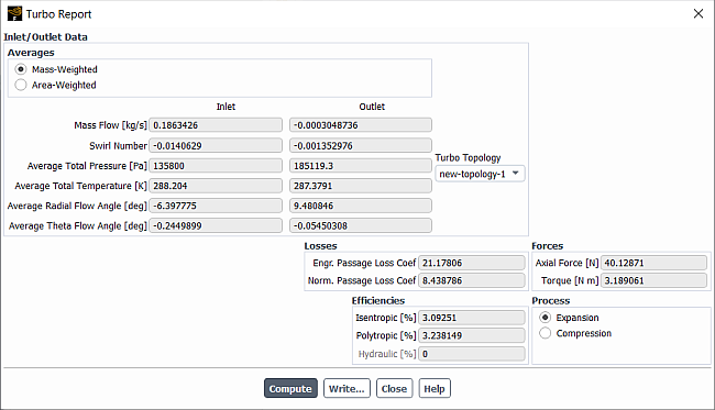
Controls
- Inlet/Outlet Data
contains quantities that can be calculated at inlets and outlets.
- Averages
allows you to choose between Mass-Weighted and Area-Weighted averages for all applicable computed quantities. These quantities are calculated for the Inlet and Outlet topologies where applicable.
- Turbo Topology
contains a list of defined topologies. Select from the list to display the values for the selected topology.
- Mass Flow
is the mass flow rate through a surface as defined in Equation 14–19.
- Swirl Number
is the swirl number as defined in Equation 14–20.
- Average Total Pressure
is the area-averaged or mass-averaged total pressure as defined in Equation 14–21 or Equation 14–22.
- Average Total Temperature
is the area-averaged or mass-averaged total temperature as defined in Equation 14–23 or Equation 14–24.
- Average Radial Flow Angle
is the area-averaged or mass-averaged radial flow angle as defined in Equation 14–25 or Equation 14–27.
- Average Theta Flow Angle
is the area-averaged or mass-averaged tangential flow angle as defined in Equation 14–26 or Equation 14–28.
- Losses
contains the values of loss-related coefficients.
- Engr. Passage Loss Coef
is the engineering loss coefficient as defined in Equation 14–29.
- Norm. Passage Loss Coef
is the normalized loss coefficient as defined in Equation 14–30.
- Forces
contains the axial force and the torque on the rotating parts.
- Axial Force
is the axial force on the rotating parts as defined in Equation 14–31.
- Torque
is the torque on the rotating parts as defined in Equation 14–32.
- Efficiencies
contains the values of isentropic, polytropic and hydraulic efficiencies.
- Isentropic
is the isentropic efficiency for a compressor or a turbine (motor) calculated in the presence of a compressible working fluid as defined in Equation 14–37 or Equation 14–43.
- Polytropic
is the polytropic efficiency for a compressor or a turbine (motor) calculated in the presence of a compressible working fluid as defined in Equation 14–38 or Equation 14–44.
- Hydraulic
is the hydraulic efficiency for a pump or a hydraulic turbine (motor) calculated in the presence of an incompressible working fluid as defined in Equation 14–33 or Equation 14–39.
- Process
specifies whether to compute the efficiency for the flow Expansion (for example, in a turbine) or Compression (for example, in a pump or compressor).
- Compute
starts the calculation of the quantities in all the fields in the Turbo Report dialog box. Note that this process may take some time for a large problem.
- Write...
opens the Select File dialog box, which you can use to save the reported values to a file.
The Turbo Topology dialog box allows you to define the topology for a turbomachinery application, so that you can use the turbomachinery-specific postprocessing features described in Turbomachinery Postprocessing. See Defining the Turbomachinery Topology for details about the items below.
![]() Domain → Mesh Models
→ Turbo Topology...
Domain → Mesh Models
→ Turbo Topology...
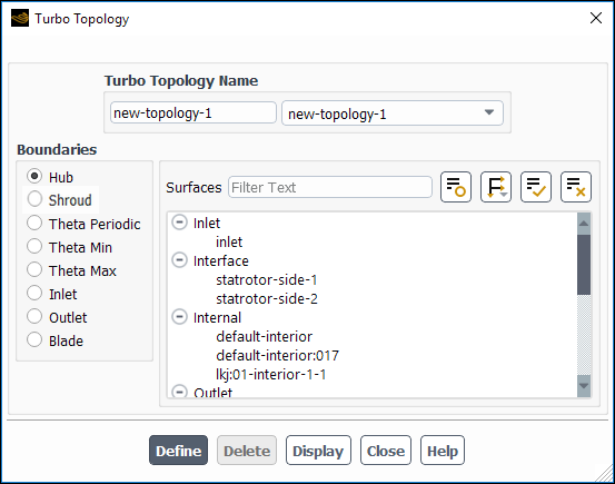
Controls
- Turbo Topology Name
specifies the name of the new topology.
- Boundaries
contains radio buttons for the topology boundaries to be defined.
- Hub
specifies the definition for the wall zone(s) forming the lower boundary of the flow passage (generally toward the axis of rotation of the machine).
- , Shroud
specifies the definition of the wall zone(s) forming the upper boundary of the flow passage (away from the axis of rotation of the machine).
- Theta Periodic
specifies the definition of the periodic boundary zone(s) on the circumferential boundaries of the flow passage.
- Theta Min, Theta Max
specify the definition of the wall zones at the minimum and maximum angular (
 ) positions on a circumferential boundary.
- Inlet
specifies the definition of the inlet zone(s) through which the flow enters the passage.
- Outlet
specifies the definition of the outlet zone(s) through which the flow exits the passage.
- Blade
specifies the definition of the wall zone(s) that defines the blade(s) (if any). Note that these zones cannot be attached to the circumferential boundaries. For this situation, use Theta Min and Theta Max to define the blade.
- Surfaces
contains a selectable list of the available surfaces, from which you can select the surface(s) that represent the boundary selected under Boundaries.
- Define
defines the new topology. If you have selected an existing topology the button is replaced by the button.
- Display
displays the defined topology in the active graphics window.
The UDF Library Manager dialog box allows you to load/unload the user-defined function libraries. See the separate Fluent Customization Manual for details.
![]() User Defined → User Defined
→ Functions → Manage...
User Defined → User Defined
→ Functions → Manage...
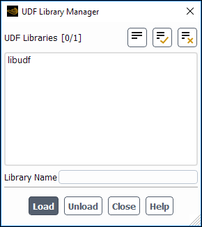
Controls
- UDF Libraries
lists the user-defined function libraries that are loaded in Ansys Fluent.
- Library Name
specifies the name of the library to be loaded/unloaded.
- Load
opens the specified library and loads the user-defined function.
- Unload
unloads the specified library.
The User-Defined Fan Model dialog box allows you to periodically regenerate a profile file that can be used to specify the characteristics of a fan, including pressure jump across the fan, and radial and swirling components of velocity generated by the fan. See User-Defined Fan Model for details about this feature and how to use this dialog box.
![]() User Defined → Model Specific
→ Fan Model...
User Defined → Model Specific
→ Fan Model...
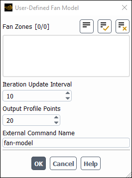
Controls
- Fan Zones
contains a list from which you can select the fan zone(s) on which your executable will operate.
- Iteration Update Interval
specifies how often the executable will be called on to update the fan profile file.
- Output Profile Points
specifies the number of points in the profile file to be written by Ansys Fluent.
- External Command Name
specifies the name of the executable.
The User-Defined Function Hooks dialog box allows you to specify user-defined functions (UDFs) connected to a number of models and procedures in Ansys Fluent. See the separate Fluent Customization Manual for details.
Important: You can hook multiple UDFs to the following functions:
Initialization
Adjust
Execute At End
Read Legacy Case
Read Case
Write Legacy Case
Write Case
Read Legacy Data
Read Data
Write Legacy Data
Write Data
Execute at Exit
![]() User Defined → User Defined
→ Function Hooks...
User Defined → User Defined
→ Function Hooks...
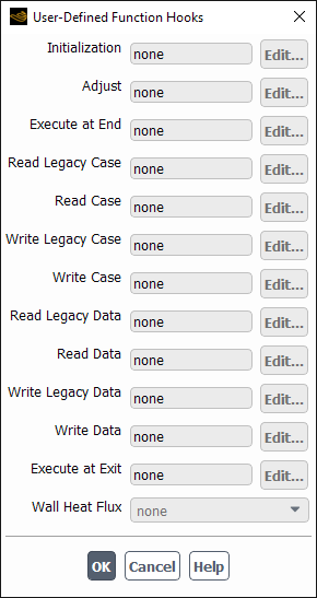
Controls
- Initialization
selects a UDF that is called immediately after you initialize your flow field.
- Adjust
selects a UDF that is called at the beginning of an iteration before solution of velocities, pressure, and other quantities begins.
- Execute At End
selects a UDF that is called at the end of an iteration or time-step.
- Read Legacy Case
selects a UDF that defines a customized section that is to be read from the legacy case file.
- Read Case
selects a UDF that defines a customized section that is to be read from the case file.
- Write Legacy Case
selects a UDF that defines a customized section that is to be written to the legacy case file.
- Write Case
selects a UDF that defines a customized section that is to be written to the case file.
- Read Legacy Data
selects a UDF that defines a customized section that is to be read from the legacy data file.
- Read Data
selects a UDF that defines a customized section that is to be read from the data file.
- Write Legacy Data
selects a UDF that defines a customized section that is to be written to the legacy data file.
- Write Data
selects a UDF that defines a customized section that is to be written to the data file.
- Execute at Exit
selects a UDF that is called when exiting an Ansys Fluent session.
- Wall Heat Flux
selects a UDF that modifies the way that the solver computes the heat flux between a wall and the neighboring fluid cells.
- Net Reaction Rate
selects a UDF that defines the net reaction rate.
- Volume Reaction Rate
selects a UDF that defines a volumetric reaction rate.
- Surface Reaction Rate
selects a UDF that defines a surface reaction rate.
- Particle Reaction Rate
selects a UDF that defines a particle reaction rate.
- Turbulent Premixed Source
selects a UDF that defines the turbulent flame speed and source term for the premixed or partially premixed combustion model.
- Chemistry Step
selects a UDF that defines the chemistry step function.
- Spray Collide
selects a UDF that defines the spray collide function.
- Cavitation Mass Rate
selects a UDF that defines the cavitation rate.
- DO Source
selects a UDF that defines the discrete ordinate source function.
- DO Diffuse Reflectivity
selects a UDF that defines the diffuse reflectivity function for the DO radiation model.
- DO Specular Reflectivity
selects a UDF that defines the specular reflectivity function for the DO radiation model.
- Emissivity Weighting Factor
selects a UDF that defines the emissivity weighting factor for the non-gray DO radiation model or the non-gray P-1 radiation model.
- Thickened Flame Model Parameters
selects a UDF that defines the parameters for the Thickened Flame Model.
The User-Defined Memory dialog box allows you to allocate memory for user-defined storage variables. See the separate Fluent Customization Manual for details.
![]() User-Defined → User Defined
→ Memory...
User-Defined → User Defined
→ Memory...
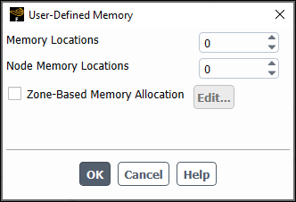
Controls
- Memory Locations
specifies the number of memory locations to be allocated.
- Node Memory Locations
specifies the number of node memory locations to be allocated.
- Zone-Based Memory Allocation
specifies that the user-defined memory will only be allocated to the specified zones, rather than the whole domain.
- Edit...
opens the Select UDM Zones Dialog Box.
Important: When writing data files in the legacy format (.dat files),
you must select the UDM quantities using the Data File Quantities
dialog box in order to postprocess them in CFD-Post. Alternatively, you have the option of
exporting the desired quantities to a .cdat file. This will
ensure that all the UDM quantities are available for postprocessing in CFD-Post. Refer to
the Ansys CFD-Post manual for more information.
![]() Solution → Reports → Definitions → New → User
Defined...
Solution → Reports → Definitions → New → User
Defined...
or
![]() Solution → Report
Definitions
Solution → Report
Definitions ![]() New
→ User Defined
New
→ User Defined
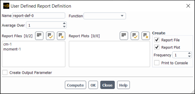
Controls
- Name
specifies the name of the report definition.
- Function
drop-down list where you can select the function that you loaded for this report definition.
- Average Over
(optional) To have Fluent calculate a running average for the User Defined Report Definition you can enter a positive integer greater than 1 (the default) for Average Over.
Specifying a number greater than 1 means that Fluent will print, plot, and write the running average value of the selected variable instead of the current value of the same variable.
The value reported is averaged over the last
iterations/time steps, where is your specified Average Over value. When
the iteration/time step number is lower than , Fluent calculates the average of the available variable
values.
- Retain Instantaneous Values
appears when Average Over is set to a value greater than
1. If enabled when you are creating a new report definition, it ensures that all instantaneous values are saved in the new report file that is being created for this report definition. It also results in the Plot Instantaneous Values option being enabled in the newly created report plot.- Report Files
lists all of the report files where you can write the report definition data.
- Report Plots
lists all of the report plots where you can plot the report definition data (assuming this report has the same units as the other report definitions included in the selected report plot).
- Create
- Report File
creates a new report file that includes this report definition.
- Report Plot
creates a new report plot that includes this report definition.
- Frequency
specifies how frequently the report definition is written, plotted, or printed to the console.
- Print to Console
prints the value of the report definition to the console.
- Create Output Parameter
creates an output parameter for this report definition with the name
<report definition name>-op.
The User-Defined Scalars dialog box allows you to include user-defined scalar transport equations in your calculation. See User-Defined Scalar (UDS) Transport Equations for details.
![]() User Defined → User Defined
→ Scalars...
User Defined → User Defined
→ Scalars...
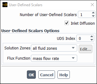
Controls
- Number of User-Defined Scalars
specifies how many additional scalar transport equations you would like to include in the calculation.
- Inlet Diffusion
when enabled allows you to include the diffusion term in the UDS transport equation for all inflow and outflow boundaries.
- User-Defined Scalars Options
contains settings that define the scalar transport equation.
- UDS Index
when set to
 marks the first user-defined scalar equation.
- Solution Zones
specifies in which zone the scalar equation will be solved: all fluid zones, all solid zones, all zones (fluid and solid) or selected zones.
- Flux Function
is a drop-down list containing available functions for the convection term of the user-defined scalar transport equation(s).
- none
(the default) indicates that there is no convection term included in the scalar transport equation(s); that is, you want to solve a Poisson equation instead of a convection/diffusion equation.
- mass flow rate
indicates that the convection term in the scalar transport equation(s) is equal to the mass flow rate
 .
.
Note that the none and mass flow rate options will apply to all solved user-defined scalars. A user-defined flux function must be supplied if a different convective flux is desired for each user-defined scalar.
- Unsteady Function
is a drop-down list containing available functions for the unsteady term of the user-defined scalar transport equation(s).
The Vectors dialog box controls the display of vector plots. See Displaying Vectors for details about the items below.
![]() Results → Graphics
→ Vectors → New...
Results → Graphics
→ Vectors → New...
Note:
The "global"/non-persistent form of graphics objects is hidden by default. If this interrupts your workflow, you can make them available by enabling the Expose legacy non-persistent graphics option in the Graphics branch of Preferences (accessed via File>Preferences...).
(When you click Edit... instead of New..., it opens the "global"/non-persistent version of the Vectors dialog box. This version of the dialog box does not have a Name field and it is not saved with the case file.
You are encouraged to use the persistent version that is accessed by clicking New....
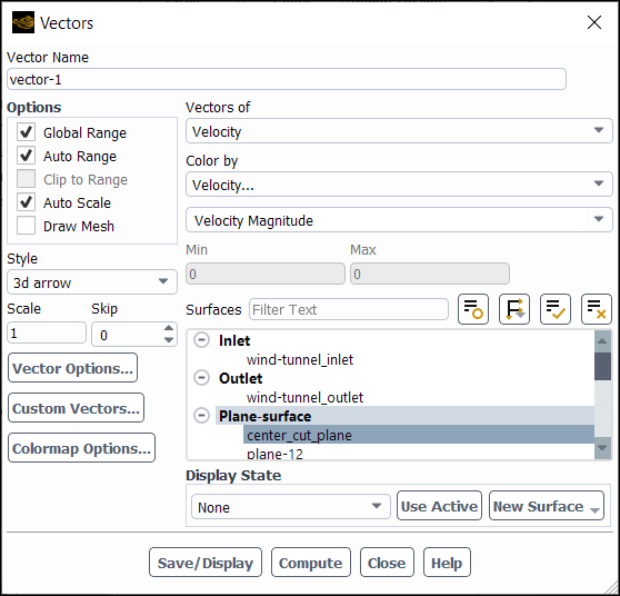
Controls
- Vector Name
is the name for a vector plot definition. You can specify a name or use the default name
vector-. This control appears only for vector plot definitions.id- Options
contains check buttons that set various display options.
- Global Range
toggles between basing the minimum and maximum values on the range of values on the selected surfaces (off), and basing them on the range of values in the entire domain (on, the default).
- Auto Range
toggles between automatic and manual setting of the range of scalar field values.
- Clip to Range
controls the display of vectors that have a value outside the range specified by Min and Max. When on, no vectors are displayed outside the range. When off, vectors are displayed outside the range using the colors at the top and bottom of the color scale. This option is applicable only when Auto Range is off. See Specifying the Range of Magnitudes Displayed for details.
- Auto Scale
enables the scaling of all vectors in the domain such that when the Scale is 1, there will be minimal overlap of vectors.
- Draw Mesh
toggles between displaying and not displaying the mesh. The Mesh Display Dialog Box is opened when Draw Mesh is selected.
- Style
selects the style in which the vectors are drawn. Available styles are 3d arrow, 3d arrowhead, cone, filled-arrow, arrow, harpoon, and headless.
- Scale
sets the factor by which the vectors should be scaled. See Scaling the Vectors for details.
- Skip
allows you to "thin" or "sample" the vectors that are displayed. See Skipping Vectors for details.
- Vector Options...
opens the Vector Options Dialog Box, in which you can set additional options for vector displays.
- Custom Vectors...
opens the Custom Vectors Dialog Box, in which you can define your own vector fields.
- Colormap Options...
opens the Colormap Dialog Box, allowing you to customize the colormap for this graphics object.
- Vectors of
contains a list from which you can select the vector field to be plotted.
- Color by
contains a list from which you can select the scalar field by which the vectors are colored.
- Phase
(Multiphase only) specifies the phase where the postprocessing operations are being applied.
- Min
shows the value to which the lower end of the color scale is mapped. You can set this value manually if Auto Range is off.
- Max
shows the value to which the upper end of the color scale is mapped. You can set this value manually if Auto Range is off.
- Surfaces
contains a list from which you can select the surfaces on which to display vectors. In 2D, vectors are displayed on the entire domain if no surface is selected.
- Display State
specifies the display state that is associated with this graphics object.
- drop-down list of display states
selectable list of all the existing display states associated with this case.
creates a display state that matches the settings of the active graphics window and assigns it to this graphics object (this association is only saved after you click ).
- New Surface
is a drop-down list button that contains a list of surface options:
- Point
opens the Point Surface Dialog Box.
- Line/Rake
opens the Line/Rake Surface Dialog Box.
- Plane
opens the Plane Surface Dialog Box.
- Quadric
opens the Quadric Surface Dialog Box.
- Iso-Surface
opens the Iso-Surface Dialog Box.
- Iso-Clip
opens the Iso-Clip Dialog Box.
- Structural Point
opens the Structural Point Surface Dialog Box.
- Display
displays the vectors in the active graphics window.
- Compute
calculates the scalar field and updates the Min and Max values (even when Auto Range is off).
- Save/Display
plots the vectors in the active graphics window and saves the vector plot definition. This button appears only for vector plot definitions and replaces the Display button.
![]() Solution → Reports
→ Definitions → New
→ Volume Report
Solution → Reports
→ Definitions → New
→ Volume Report
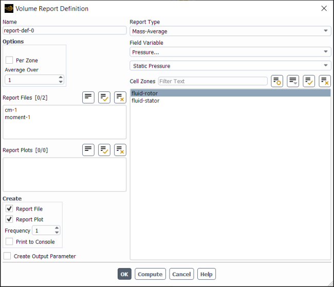
Controls
- Name
specifies the name of the report definition.
- Options
- Per Zone
specifies whether or not the chosen field variable is calculated from all of the selected cell zones combined (default) or individually on each of the selected cell zones.
- Average Over
(optional) To have Fluent calculate a running average for the Volume Report Definition you can enter a positive integer greater than 1 (the default) for Average Over.
Specifying a number greater than 1 means that Fluent will print, plot, and write the running average value of the selected variable instead of the current value of the same variable.
The value reported is averaged over the last
iterations/time steps, where is your specified Average Over value.
When the iteration/time step number is lower than , Fluent calculates the average of the available variable
values.
- Retain Instantaneous Values
appears when Average Over is set to a value greater than
1. If enabled when you are creating a new report definition, it ensures that all instantaneous values are saved in the new report file that is being created for this report definition. It also results in the Plot Instantaneous Values option being enabled in the newly created report plot.
- Report Files
lists all of the report files where you can write the report definition data.
- Report Plots
lists all of the report plots where you can plot the report definition data (assuming this report has the same units as the other report definitions included in the selected report plot).
- Create
- Report File
creates a new report file that includes this report definition.
- Report Plot
creates a new report plot that includes this report definition.
- Frequency
specifies how frequently the report definition is written, plotted, or printed to the console.
- Print to Console
prints the value of the report definition to the console.
- Create Output Parameter
creates an output parameter for this report definition with the name
<report definition name>-op.- Report Type
selects the integration method used on the selected cell zones. The available report types are the same as those in the Volume Integrals Dialog Box. See Volume Integration for details.
- Field Variable
contains a list of solution variables that can be monitored on the selected cell zones. This list will not be available if you select Volume as the Report Type.
- Phase
contains a list of all of the phases in the problem that you have defined. This is available when the VOF, mixture, or Eulerian multiphase model is enabled.
- Cell Zones
contains a selectable list of the current cell zones.
- OK
creates the report definition.
- Compute
computes the value of the report definition at the selected zone(s) and prints to the console.
The Warning dialog box allows you to specify whether existing dynamic zones and/or mesh interfaces are deleted when you are using the Merge Zones dialog box to merge multiple zones of the same type into a single zone (see Merge Zones Dialog Box for details). Note that dynamic zones and mesh interfaces that exist at the time of the merge may be adversely affected by the merge.
The Warning dialog box opens automatically when you click in the Merge Zones Dialog Box if your case has dynamic zones or mesh interfaces.
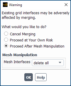
Controls
- Cancel Merging
returns you to the Mesh Zones dialog box when you click , without initiating the merge.
- Proceed at Your Own Risk
allows the merge to proceed when you click , without deleting the existing dynamic zones and mesh interfaces beforehand.
- Proceed After Mesh Manipulation
deletes the existing dynamic zones and/or mesh interfaces (based on the settings in the Mesh Manipulation group box) and then merges the zones when you click .
- Mesh Manipulation
allows you to specify whether the existing dynamic zones and/or mesh interfaces are deleted prior to the initiation of the merge. This group box is only available when Proceed After Mesh Manipulation is selected.
- Dynamic Zones
specifies whether all existing dynamic zones are deleted prior to the merge.
- Mesh Interfaces
specifies whether all existing mesh interfaces are deleted prior to the merge.
Note that selecting keep all from both drop-down lists in the Mesh Manipulation group box is the equivalent of selecting Proceed at Your Own Risk.
The Zone Surface dialog box allows you to interactively create surfaces from face and cell zones in the domain. See Zone Surfaces for details about the items below.
![]() Domain → Surface
→ Create → Zone...
Domain → Surface
→ Create → Zone...
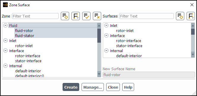
Controls
- Zone
lists zones that you can select for creating zone surfaces.
- Surfaces
displays an informational list of existing surfaces.
- New Surface Name
designates the name of the surface to be created. The default is the zone name.
- Create
creates the surface.
- Manage...
opens the Surfaces Dialog Box in which you can rename and delete surfaces and determine their sizes.
The Zone Type Color and Material Assignment dialog box allows you to control the mesh coloring for meshes displayed using the Displaying the Mesh with By Type selected for Coloring. It is opened by clicking next to By Type in the Mesh Display Dialog Box See Zone Surfaces for details about the items below.
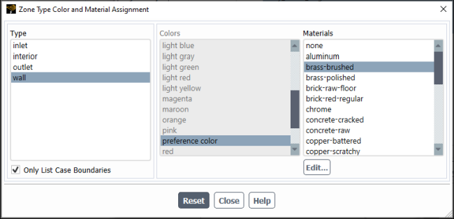
Controls
- Type
contains a selectable list of zone types. Select a Type to set its color and/or material.
- Only List Case Boundaries
limits the Type list to only include zone types that are included in the current case file.
- Colors
lists the available colors that may be used to color the selected zone type.
- Materials
lists the available materials that may be used to color the selected zone type. Click if you want to modify a material's color. See Creating Custom Realistic Materials for additional information.
opens the Material Editor Dialog Box.
- Reset
resets the mesh colors and material assignments to the default selections for all zone types.