


Solution of the discrete phase implies integration in time of the force balance on the particle (Equation 12–1 in the Theory Guide) to yield the particle trajectory. As the particle is moved along its trajectory, heat and mass transfer between the particle and the continuous phase are also computed via the heat/mass transfer laws (Laws for Heat and Mass Exchange in the Theory Guide). The accuracy of the discrete phase calculation therefore depends on the time accuracy of the integration and upon the appropriate coupling between the discrete and continuous phases when required. Numerical controls are described in Numerics of the Discrete Phase Model. Coupling and performing trajectory calculations are described in Performing Trajectory Calculations. Resetting the Interphase Exchange Terms and Parallel Processing for the Discrete Phase Model provide information about resetting interphase exchange terms and using the parallel solver for a discrete phase calculation.
For additional information, see the following sections:
The trajectories of your discrete phase injections are computed when you display the trajectories using graphics or when you perform solution iterations. That is, you can display trajectories without impacting the continuous phase, or you can include their effect on the continuum (termed a coupled calculation). In turbulent flows, trajectories can be based on mean (time-averaged) continuous phase velocities or they can be impacted by instantaneous velocity fluctuations in the fluid. This section describes the procedures and commands you use to perform coupled or uncoupled trajectory calculations, with or without stochastic tracking.
For the uncoupled calculation, you will perform the following two steps:
Solve the continuous phase flow field.
Plot (and report) the particle trajectories for discrete phase injections of interest.
In the uncoupled approach, this two-step procedure completes the modeling effort, as illustrated in Figure 24.56: Uncoupled Discrete Phase Calculations. The particle trajectories are computed as they are displayed, based on a fixed continuous-phase flow field. Graphical and reporting options are detailed in Postprocessing for the Discrete Phase.
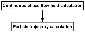
This procedure is adequate when the discrete phase is present at a low mass and momentum loading, in which case the continuous phase is not impacted by the presence of the discrete phase.
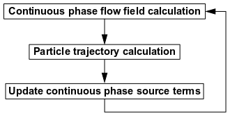
In a coupled two-phase simulation, Ansys Fluent modifies the two-step procedure above as follows:
Solve the continuous phase flow field (prior to introduction of the discrete phase).
Introduce the discrete phase by calculating the particle trajectories for each discrete phase injection.
Recalculate the continuous phase flow, using the interphase exchange of momentum, heat, and mass determined during the previous particle calculation.
Recalculate the discrete phase trajectories in the modified continuous phase flow field.
Repeat the previous two steps until a converged solution is achieved in which both the continuous phase flow field and the discrete phase particle trajectories are unchanged with each additional calculation.
This coupled calculation procedure is illustrated in Figure 24.57: Coupled Discrete Phase Calculations. When your Ansys Fluent model includes a high mass and/or momentum loading in the discrete phase, the coupled procedure must be followed in order to include the important impact of the discrete phase on the continuous phase flow field.
Important: When you perform coupled calculations, all defined discrete phase injections will be computed. You cannot calculate a subset of the injections you have defined. If there are massless particle injections defined, these will have no effect in the coupled calculation.
If your Ansys Fluent model includes prediction of a coupled two-phase flow, you should begin with a partially (or fully) converged continuous-phase flow field. You will then create your injection(s) and set up the coupled calculation.
For each discrete-phase iteration, Ansys Fluent computes the particle/droplet trajectories and updates the interphase exchange of momentum, heat, and mass in each control volume. These interphase exchange terms then impact the continuous phase when the continuous phase iteration is performed. During the coupled calculation, Ansys Fluent will perform the discrete phase iteration at specified intervals during the continuous-phase calculation. The coupled calculation continues until the continuous phase flow field no longer changes with further calculations (that is, all convergence criteria are satisfied). When convergence is reached, the discrete phase trajectories no longer change either, since changes in the discrete phase trajectories would result in changes in the continuous phase flow field.
The steps for setting up the coupled calculation are as follows:
Solve the continuous phase flow field.
In the Discrete Phase Model Dialog Box (Figure 24.1: The Discrete Phase Model Dialog Box - Tracking Tab), enable the Interaction with Continuous Phase option.
Set the frequency with which the particle trajectory calculations are introduced in the DPM Iteration Interval field. If you set this parameter to 5, for example, a discrete phase iteration will be performed every fifth continuous phase iteration. The optimum number of iterations between trajectory calculations depends upon the physics of your Ansys Fluent model.
Important: Note that if you set this parameter to 0, Ansys Fluent will not perform any discrete phase iterations.
During the coupled calculation (which you initiate using the Run Calculation Task Page in the usual manner) you will see the following information in the Ansys Fluent console as the continuous and discrete phase iterations are performed:
iter   continuity   x-velocity   y-velocity       k         epsilon       energy    time/it
 314   2.5249e-01   2.8657e-01   1.0533e+00   7.6227e-02   2.9771e-02   9.8181e-03   :00:05
 315   2.7955e-01   2.5867e-01   9.2736e-01   6.4516e-02   2.6545e-02   4.2314e-03   :00:03

  DPM  Iteration  ....
  number  tracked=  9,  number  escaped=  1,  aborted=  0,  trapped=  0,  evaporated  =  8,i
Done.
 316   1.9206e-01   1.1860e-01   6.9573e-01   5.2692e-02   2.3997e-02   2.4532e-03   :00:02
 317   2.0729e-01   3.2982e-02   8.3036e-01   4.1649e-02   2.2111e-02   2.5369e-01   :00:01
 318   3.2820e-01   5.5508e-02   6.0900e-01   5.9018e-02   2.6619e-02   4.0394e-02   :00:00
Note that you can perform a discrete phase calculation at any
time by using the solve/dpm-update text command.
If you include the stochastic prediction of turbulent dispersion in the coupled two-phase flow calculations, the number of stochastic tries applied each time the discrete phase trajectories are introduced during coupled calculations will be equal to the Number of Tries specified in the Set Injection Properties Dialog Box. For transient particle tracking, the number of tries is set to 1. Input of this parameter is described in Stochastic Tracking. An input of  requests
  stochastic trajectory calculations for each particle in the injection. When the number of stochastic tracks included is small, you may find that the ensemble average of the trajectories is quite different each time the trajectories are computed. These differences may, in turn, impact the convergence of your coupled solution. For good convergence of a coupled solution, a statistical independent distribution of tracks can be achieved with an adequate number of stochastic tracks and/or a sufficient number of different starting locations of the tracks.
When you are coupling the discrete and continuous phases using the calculation procedures noted above, Ansys Fluent applies under-relaxation to the momentum, heat, and mass transfer terms. This under-relaxation serves to increase the stability of the coupled calculation procedure by letting the impact of the discrete phase change only gradually:
 | (24–14) |
where  is
the exchange term,
is
the exchange term,  is
the previous value,
is
the previous value,  is the newly computed value,
and
is the newly computed value,
and  is the particle/droplet under-relaxation
factor. For
is the particle/droplet under-relaxation
factor. For  , Ansys Fluent uses a default value of 0.5 for
all types of analysis except transient flows with unsteady particle
tracking, in which case the default value of 0.9 is used. You can
modify
, Ansys Fluent uses a default value of 0.5 for
all types of analysis except transient flows with unsteady particle
tracking, in which case the default value of 0.9 is used. You can
modify  by changing the value in the Discrete Phase Sources field under Under-Relaxation
Factors in the Solution Controls task
page. You may need to decrease
by changing the value in the Discrete Phase Sources field under Under-Relaxation
Factors in the Solution Controls task
page. You may need to decrease  in order to improve the stability of coupled
discrete phase calculations.
in order to improve the stability of coupled
discrete phase calculations.
Figure 24.58: Effect of Number of Source Term Updates on Source Term Applied
to Flow Equations shows how the source term  , when applied to the flow equations, changes with the number of updates for
varying under-relaxation factors . Each DPM iteration starts with an initial
, when applied to the flow equations, changes with the number of updates for
varying under-relaxation factors . Each DPM iteration starts with an initial  value for the source term, which is typically zero at the beginning of the
calculation. After a number of updates, the source term reaches its final
value for the source term, which is typically zero at the beginning of the
calculation. After a number of updates, the source term reaches its final  value.
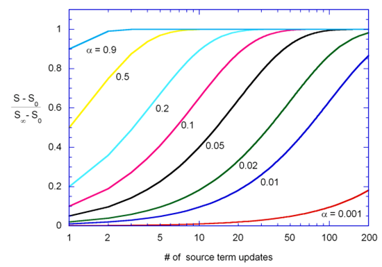
Suppose that in a continuous flow simulation with continuous DPM tracking, the DPM under-relaxation factor is chosen to be 0.5, with 20 continuous phase iterations per DPM iteration. From Figure 24.58: Effect of Number of Source Term Updates on Source Term Applied to Flow Equations, we see that approximately 10 source term updates are required for the DPM sources to reach their final values. Therefore, in this example, at least 200 continuous phase iterations are required after any change to the DPM sources (for example, a new injection or a changed DPM mass flow rate), to ensure that the change has taken effect.
For cases with convergence difficulties, reducing the under-relaxation factors is often
necessary in order to improve the stability of the coupled DPM simulation. However, for small
values of , many iterations may be needed for the DPM source to reach the final
value. You can use a text command that linearly ramps up the DPM source term
to its maximum value. At the end of each iteration  , the source term is computed as:

With this approach, even small values for under-relaxation factors can be applied, and
the final value can be reached within a reasonable iteration count. For the above
example, a minimum of two source term updates is required to reach the final values.
Accordingly, it will take only 40 continuous phase iterations to fully account for the effect
of the DPM source changes.
To use the linear growth of DPM source term functionality, use the following text commands:
define/models/dpm/interaction/linear-growth-of-dpm-source-term?
Change the DPM source term linearly every DPM iteration [no] y
Note that the impact of this option is case dependent.
If you have performed coupled calculations, resulting in nonzero interphase sources/sinks of momentum, heat, and/or mass that you do not want to include in subsequent calculations, you can reset these sources to zero.
![]() Solution
→ Initialization
Solution
→ Initialization![]() Reset DPM
Sources
Reset DPM
Sources
When you select Reset DPM Sources, the sources will immediately be reset to zero without any further confirmation from you.
The randomization of particle trajectories is used in the following models for particle injection and tracking:
random surface injection
Rosin-Rammler injection diameter distribution
volume injection
axial or radial staggering of injections
atomizer injections
cone injection direction
temporal staggering of injections
random breakup diameters (for example, from the TAB breakup model)
particle stochastic collision models
stochastic tracking in turbulent flows
Brownian motion model
Random number generators used for particle tracking are initialized (that is, seeded on individual particles) and carried with the particles to make results independent of parallel partitioning.
Often there are not enough trajectories to obtain continuous flow sources independent from the seed of the random number generator. Therefore, by default, the initialization of the random number generators is done based on the fluid flow iteration and/or particle time step, thus increasing the variation of starting conditions within the given injection parameters.
You can use the following text commands to modify the default initialization of the random number generators:
For steady cases, or when computing the same unsteady particle time step multiple times (that is, executing multiple iterations within a flow time step), the initialized injected particles will be repeated with the same random number sequence when you issue the following text command:
define/models/dpm/injections/re-randomize-every-iteration?Update randomness every iteration? [yes]nThis allows to lower the values of the fluid flow residuals because the trajectories and sources will vary by a smaller amount. The downside of this approach is that the result is more dependent on variations in the number of trajectories and on slight changes in the mesh. As an alternative for reducing oscillations in the source terms, the under-relaxation factor of DPM sources can be reduced at the cost of doing more iterations to converge.
For cases with unsteady particle tracks, you can also use the following text command to inject particles using the same random numbers in each particle time step:
define/models/dpm/numerics/re-randomize-every-timestep?Update randomness every timestep? [yes]n
Table 24.6: Randomization of Particle Trajectories in Steady and Unsteady Cases summarizes the effect of these two settings on cases with unsteady particles.
Table 24.6: Randomization of Particle Trajectories in Steady and Unsteady Cases
| Setting / Action | Value / Effect | |||
|---|---|---|---|---|
re-randomize-every-iteration | yes (default) | no | yes | no |
re-randomize-every-timestep | yes (default) | yes | no | no |
| Different random number generator initialization when injecting steady particles within the different DPM updates | yes | no | yes | no |
| Different random number generator initialization when injecting unsteady particles within the same (repeated [a]) particle time step | no | no | yes | no |
| Same random number generator initialization when injecting unsteady particles in different particle time step | no | no | no, except for different particle time steps within the same DPM update [b] | yes |
[a] Particle time steps are tracked repeatedly if more than one DPM update is done within the same flow time step. This happens when the specified DPM Iteration Interval is lower than the number of flow iterations actually executed within the flow time step.
[b] This happens when the specified particle time step is smaller than the flow time step.