The Spalart-Allmaras model is a relatively simple one-equation model that solves a modeled transport equation for the kinematic eddy (turbulent) viscosity. The Spalart-Allmaras model was designed specifically for aeronautics and aerospace applications involving wall-bounded flows and has been shown to give good results for boundary layers subjected to adverse pressure gradients. It is also gaining popularity in turbomachinery applications. Do not use the model as a general purpose model, as it is not well calibrated for free shear flows (large errors for example, jet flows).

The Spalart-Allmaras model has been extended within Ansys Fluent with a -insensitive wall treatment, which automatically blends all solution variables from their viscous sublayer formulation to the corresponding logarithmic layer values depending on . The blending is calibrated to also cover intermediate values in the buffer layer

Two-equation models are historically the most widely used turbulence models in industrial CFD. They solve two transport equations and model the Reynolds Stresses using the Eddy Viscosity approach. The standard - model in Ansys Fluent falls within this class of models and has become the workhorse of practical engineering flow calculations in the time since it was proposed by Launder and Spalding [84]. Robustness, economy, and reasonable accuracy for a wide range of turbulent flows explain its popularity in industrial flow and heat transfer simulations.

The draw-back of some - models is their insensitivity to adverse pressure gradients and boundary layer separation. They typically predict a delayed and reduced separation relative to observations. This can result in overly optimistic design evaluations for flows that separate from smooth surfaces (for example, aerodynamic bodies, diffusers). The - model is therefore not widely used in external aerodynamics.

In Ansys Fluent, the use of the Realizable - model is recommended relative to other variants of the - family. You should use the - model in combination with either the Enhanced Wall Treatment (EWT-) or the Menter-Lechner near-wall treatment. For details, refer to Enhanced Wall Treatment ε-Equation (EWT-ε) or Menter-Lechner ε-Equation (ML-ε) in the Theory Guide, respectively. For cases where the flow separates under adverse pressure gradients from smooth surfaces (airfoils, and so on), - models are generally not recommended.

The -equation offers several advantages relative to the -equation. The most prominent one is that the equation can be integrated without additional terms through the viscous sublayer. This makes the formulation of a robust -insensitive treatment relatively straightforward. Refer to y+-Insensitive Near-Wall Treatment for ω-based Turbulence Models in the Theory Guide for details. Furthermore, - models are typically better at predicting adverse pressure gradient boundary layer flows and separation. The downside of the standard -equation is a relatively strong sensitivity of the solution depending on the freestream values of and outside the shear layer. The use of the standard - model is, for this reason, not generally recommended in Ansys Fluent.

The BSL and SST - models have been designed to avoid the freestream sensitivity of the standard - model, by combining elements of the -equation and the -equation. In addition, the SST model has been calibrated to accurately compute flow separation from smooth surfaces. Within the - model family, it is therefore recommended to use either the BSL or SST model. These models are some of the most widely used models for aerodynamic flows. They are typically somewhat more accurate in predicting the details of the wall boundary layer characteristics than the Spalart-Allmaras model.

The BSL and SST models (like all other -equation based models) use a -insensitive wall treatment. For details on the available options, see y+-Insensitive Near-Wall Treatment for ω-based Turbulence Models in the Fluent Theory Guide.

Note that the turbulence default option as of Fluent 2020 R1, the - SST model, provides low levels of eddy viscosity (compared to -) and hence can predict physical phenomenon such as separation more accurately, although this may make it less stable in some cases and some solver settings may need to be updated for proper convergence.

For the - models, so-called low Reynolds number terms (low Re) have been proposed by Wilcox. These are available in Ansys Fluent as an option. It is important to point out that these terms are not required for integrating the equations through the viscous sublayer. Their main influence lies in mimicking laminar-turbulent transition processes. However, this functionality is not widely calibrated and for wall-boundary layer transition, the combination of the SST model with the Transition SST model (Transition SST Model in the Theory Guide), Intermittency Transition Model (Intermittency Transition Model in the Theory Guide), or the Transition -- model (k-kl-ω Transition Model in the Theory Guide) is more reliable. The use of the low-Re terms is therefore not encouraged.

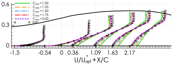
The goal of the GEKO model is to offer a single model with enough flexibility to cover a wide range of applications. Although most applications are already covered by the default settings, the model provides four free parameters that can be adjusted for specific types of applications, without negative impact on the basic calibration of the model. This is a powerful tool for model optimization, but requires a proper understanding of the impact of these coefficients to avoid mistuning. It is important to emphasize that the model has strong defaults, so you can also apply the model without any fine-tuning and that you should make sure that any tuning is supported by high-quality experimental data.

In most cases, you need to only adjust to change the GEKO model’s sensitivity to boundary layer separation. The figure below shows the impact of this parameter for a diffuser flow [39]. With , the model behaves essentially the same as the model (no separation) and with , close to perfect agreement with the data is achieved (like the SST model [99]). Larger values for can be required (for example, when simulating high-lift airfoils, where even the SST model tends to under-estimate separation strength).

Figure 15.1: Velocity Profiles for Axi-symmetric Diffuser Flow (Case CS0 – Driver). Impact of Variation of

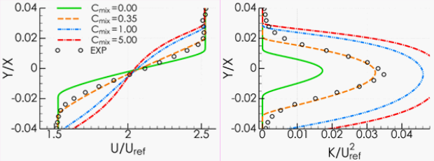
The figure below shows variations of for a free mixing layer () [18]. Increasing leads to increased turbulence levels and larger spreading rates.

Figure 15.2: Impact of Changes in on Free Mixing Layer. Left: Velocity Profiles, Right: Turbulence Kinetic Energy Profiles

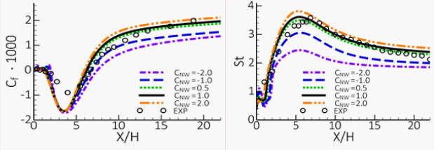
The impact of is shown in the figure below for the reattachment region of a backward-facing step [166]. Both the wall shear stress coefficient and the Stanton number for heat transfer, , are strongly affected. Increasing leads to higher and numbers in this non-equilibrium region. In most cases, there is no need to change from its default value.

Figure 15.3: Impact of Changes in on Backward Facing Jet with Heat Transfer. Left: Wall Shear Stress Coefficient, , Right: Wall Heat Transfer Coefficient,

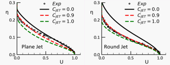
The figure below shows the influence of for plane [23] and round jet flows [174](=2, =0.35, =0.5). Increasing (while is active) reduces the spreading rate for jet flows without changing the spreading rate of mixing layers. is a sub-model of and therefore loses its effectiveness in cases where is reduced.

Figure 15.4: Impact of Changes in on Free Jet Flows. Left: Plane Jet, Right: Round Jet

Note that the region where is active is defined by the blending function . In regions where =1 (near walls) there is no effect when changing . can be visualized in Postprocessing. It can also be augmented by the modification of expert parameters (see Generalized k-ω  (GEKO) Model in the Fluent Theory Guide) or by over-writing the function via a UDF (see DEFINE_KW_GEKO Coefficients and Blending Function in the Fluent Customization Manual).

The GEKO model (like all other -equation based models) uses a -insensitive wall treatment. For details on the available options, see y+-Insensitive Near-Wall Treatment for ω-based Turbulence Models in the Fluent Theory Guide.

Reynolds Stress models (RSM) include several effects that are not easily handled by Eddy-Viscosity models. The most important effect is the stabilization of turbulence due to strong rotation and streamline curvature (as observed for example, in cyclone flows). RSM on the other hand often demand a significant increase in computing time partly due to the additional equations but mostly due to reduced convergence. This additional effort is not always justified by increased accuracy. Their usage is therefore not generally recommended and should be restricted to flows for which their superiority has been established, especially flow with strong swirl and rotation. If wall boundary layers are important, the combination of RSM with the - or BSL-equation is more accurate than the combination with the -equation. The combination of RSM with BSL removes the free-stream sensitivity observed with the -equation in the same way as for two-equation models.

Ansys Fluent also offers an algebraic Reynolds Stress Model (EARSM) which represents an extension of the standard two-equation models and is therefore a good compromise between capturing additional flow effects and computational costs.

The following four models for transition prediction are available in Ansys Fluent. Three of them can be combined with the scale-resolving methods described in Scale-Resolving Simulation (SRS) Models.

For many test cases, the four models produce similar results. Due to their combination with the SST model, the Transition SST model, the Intermittency Transition model, and the Alg- model are recommended over the Transition -- model. The Transition SST model is not Galilean invariant, and should therefore not be applied to surfaces that move relative to the coordinate system for which the velocity field is computed; furthermore, it is not suitable for fully developed pipe / channel flows where no freestream is present. For such cases, the Intermittency Transition model or the Alg- should be used instead (though you may need to adjust the Intermittency Transition model for pipe / channel flows by modifying the underlying correlations). Among the availble models, only the Intermittency Transition model is capable of accounting for crossflow instability.

The first three models belong to the class of "Local-Correlation based Transition Models" (LCTM). They model the transitional processes through inclusion of transition correlations. The performance of the models is similar for the generic test cases used in their calibration. However, since laminar-turbulent transition is a complex and highly sensitive process, the models can produce different results for complex cases.

The Transition SST model (- model) solves two additional transport equations (in addition to the underlying turbulence model). The Intermittency Transition model solves only one additional transport equation and the Alg- model solves none. Avoiding additional transport equations saves computational effort and was the main motivation for the development of these models.

The Transition SST model is the most widely used model, especially in Aeronautics, where it has become a standard RANS transition model in the last decade. However, the Intermittency Transition model has also gained acceptance due to its simpler formulation and its Galilean invariance. The Alg- model is the latest addition and is less established. However, it has also shown strength in industrial simulations where transition is often defined by geometric features and/or laminar bubbles. This model is also Galilean invariant and can be applied in any coordinate system. The optimal choice depends on the application and it is recommended to run cases with all three models and compare which model provides the best ratio of computational cost versus accuracy.

The Transition -- model is not being actively developed but has also found useful applications. Since it is only combined with the standard k- model it is not recommended as the default model.

When using these models, note the following:

One weakness of the eddy-viscosity models is that these models are insensitive to streamline curvature and system rotations, which play an important role in many turbulent flow applications. To sensitize the standard eddy-viscosity models to these curvature effects, you can use a modified turbulence production term. For more information, see Curvature Correction for the Spalart-Allmaras and Two-Equation Models in the Fluent Theory Guide.

Eddy-viscosity models have a tendency to over-predict corner flow separation zones. A simplified quadratic non-linear algebraic extension for the Spalart-Allmaras and two-equation models based on the transport equation of the specific dissipation rate ω has been implemented that drives momentum into the corner and can thus reduce corner separation effects. For more information, see Corner Flow Correction in the Fluent Theory Guide.

A disadvantage of standard two-equation turbulence models is the excessive generation of the turbulence energy, , in the vicinity of stagnation points. In order to avoid the buildup of turbulent kinetic energy in the stagnation regions, the production term in the turbulence equations can be limited by one of the two formulations described in Production Limiters for Two-Equation Models in the Fluent Theory Guide.

There are many model enhancements available for turbulence models. While such enhancements can improve simulations in some cases, they can also have detrimental effects. The general recommendation is therefore to use them with caution.

As noted above, the use of low-Re terms in combination with the -equation is not generally recommended.

Another model enhancement that should be used with care is the compressibility effects of Sarkar ([136]). It can improve the prediction of free shear layers at high Mach numbers, but has also shown a pronounced negative impact on wall boundary layers. It is therefore not generally recommended. The compressibility effects option is available in the Viscous Model Dialog Box when the compressible form of the ideal gas law or the real-gas model is enabled. This option is disabled by default (though this was not the case in version 14.5 and earlier) and it is recommended that you keep this option disabled for cases not involving free shear flows.

Buoyancy has a pronounced effect on turbulence (Effects of Buoyancy on Turbulence in the Theory Guide). The use of the source term in the -equation is therefore recommended for buoyancy affected flows. The source term in the -equation and -equation is much less established and the term should be enabled with care.

It is recommended that you use a -insensitive wall treatment for all models for which it is available (Spalart-Allmaras, -equation and -equation). It provides the most consistent wall shear stress and wall heat transfer predictions with the least sensitivity to values. (See an Overview of the Spalart-Allmaras model, Enhanced Wall Treatment ε-Equation (EWT-ε), Menter-Lechner ε-Equation (ML-ε), and y+-Insensitive Near-Wall Treatment for ω-based Turbulence Models in the Theory Guide for more information.)

When Wall Functions are used, it is necessary to avoid grids with fine near wall spacing. It is recommended that you use in the entire domain. The application of Wall Functions is, however, not generally recommended as they do not allow a systematic refinement of the near wall grid. Wall Functions are especially damaging for flows at low to medium Reynolds numbers (Re~-), as the assumption of an extended logarithmic layer is not valid in these cases. In case that Wall Functions are desired, the option of Scalable Wall Functions (Scalable Wall Functions in the Theory Guide) avoids the grid restrictions and can be run on fine meshes.

Grid generation has a strong impact on model accuracy. There are many considerations that have to be followed when generating high quality CFD grids. From a turbulence modeling standpoint, the most important one is that the relevant shear layers should be covered by at least ~10 cells normal to the layer. Below this resolution, the model will not be able to provide its calibrated performance. Especially for free shear flows, whose location is not known during grid generation, this is a requirement that is hard to achieve. Nevertheless, you should be aware that for lower resolution, the model performance can degrade.

For wall bounded flows, a structured mesh in wall-normal direction is highly recommended. The structured portion of the mesh should cover the entire boundary layer and extend beyond the boundary layer thickness to avoid restricting the growth of the boundary layer. Advanced turbulence models for wall boundary layers like the Spalart-Allmaras model and the SST model will only provide improved results to other models if a minimum of 10 or more structured (hex or prism) cells are located inside the boundary layer. In addition, one should ensure that the prism layer covers the wall boundary layer entirely. Note that these are not specific requirements of these models, but are general requirements for wall boundary layer simulations.

Both ε-based and ω-based models offer -insensitive wall treatment options (see Enhanced Wall Treatment ε-Equation (EWT-ε), Menter-Lechner ε-Equation (ML-ε), and y+-Insensitive Near-Wall Treatment for ω-based Turbulence Models in the Theory Guide for more information), which make the models relatively insensitive to the -value of the wall cell. Generally speaking, it is more important to ensure that the boundary layer is covered with sufficient cells, then to achieve a certain criterion. However, for simulations with high accuracy demands on the wall boundary layer (especially for heat transfer predictions), near-wall meshes with ~1 are recommended. When wall functions are used, it is essential to avoid meshes with values lower than ~30 as the wall shear stress and the wall heat transfer can and will seriously deteriorate under such conditions. For this reason, the usage of -insensitive wall treatments (to be selected for -equation and default for -equation based models) is recommended.

For transition models (see k-kl-ω Transition Model, Transition SST Model, and Intermittency Transition Model in the Theory Guide), more stringent grid resolution requirements apply than for standard RANS models, as transition modeling requires the resolution of the thin laminar boundary layer upstream of the transition location. For this reason, a low-Re mesh () with sufficient streamwise resolution is needed to accurately resolve the transition region. The expansion ratio of the grid normal to the wall should not exceed 1.1. Furthermore, in regions where laminar separation occurs, additional mesh refinement is necessary, in order to properly capture the rapid transition due to the separation bubble. Finally, the decay of turbulence from the inlet to the leading edge of the device should always be estimated before running a solution as this can have a large effect on the predicted transition location.

The most widely known SRS modeling concept is Large Eddy Simulation (LES). It is based on the approach of resolving large turbulent structures in space and time down to the grid limit everywhere in the flow. However, while widely used in the academic community, LES had very limited impact on industrial simulations. The reason lies in the excessively high resolution requirements for wall boundary layers. Near the wall, the largest scales in the turbulent spectrum are nevertheless geometrically very small and require a very fine grid and a small time step size. In addition, unlike RANS, the grid cannot only be refined in the wall normal direction, but also must resolve turbulence in the wall parallel plane. This can only be achieved for flows at very low Reynolds number and on very small geometric scales (the extent of the LES domain cannot be much larger than 10-100 times the boundary layer thickness parallel to the wall). For this reason the use of LES is only recommended for flows where wall boundary layers are not relevant and need not be resolved or for flows where the boundary layers are laminar due to the low Reynolds number. In such cases, the most balanced LES model is the WALE model (see Wall-Adapting Local Eddy-Viscosity (WALE) Model in the Theory Guide). It offers a good compromise between model complexity and generality. It also allows computing laminar shear (boundary) layers without any model impact.

An extension to LES is Wall-Modeled LES (WMLES). It allows the LES computation of wall bounded flows at higher Reynolds number without the large increase in grid resolution required for conventional LES at high Reynolds numbers. For WMLES, the grid resolution is largely independent of the Reynolds number with respect to the grid cells required per boundary layer volume. An enhanced version of WMLES called WMLES - is also available. WMLES does not provide zero eddy-viscosity for flows with constant shear. Therefore, it does not allow the computation of transitional effects, and can produce overly large eddy-viscosities in separating shear layers. The enhanced WMLES - formulation overcomes these deficiencies. See Algebraic Wall-Modeled LES Model (WMLES) in the Theory Guide for further details.

In order to avoid the high resolution requirements of LES, numerous hybrid models have been developed in recent years. These are models that combine certain elements of RANS and LES approaches in a way that allows for the simulation of high Reynolds number flows. With hybrid models, the attached wall boundary layers are typically covered by the RANS part of the model, while large detached regions are handled in ‘LES’ mode, meaning with a partial resolution of the turbulent spectrum in space and time. Hybrid models rely on a strong enough flow instability to generate turbulent structures in the separated zone. This is typically the case for flows behind bluff bodies, where URANS models predict single-mode periodic vortex shedding. Hybrid models allow these vortices to generate smaller eddies down to the available grid limit. Figure 15.5: Illustration of SST-URANS vs. SST-SAS Models shows a typical scenario: While the application of a standard RANS model in unsteady mode results in a single frequency vortex shedding (left), the application of hybrid models allows a break-up of the large structures into smaller scales. This is beneficial for predicting the correct mixing behind the body or to extract spectral information (for example, for acoustic simulations). At the same time, the wall boundary layers are covered by the RANS part of the hybrid model avoiding the excessive resolution requirements of LES.

Figure 15.5: Illustration of SST-URANS vs. SST-SAS Models

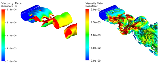
Figure 15.5: Illustration of SST-URANS vs. SST-SAS Models shows a circular cylinder in a cross flow at . The left hand side illustrates the SST-URANS model, while the right-hand side illustrates the SST-SAS model. The isosurface of is colored according to the eddy viscosity ratio (note that the scale in the right-hand side figure is smaller by a factor of 14).

 

15.2.2.2.1. Scale-Adaptive Simulation (SAS)

The SAS modeling approach (see Scale-Adaptive Simulation (SAS) Model in the Theory Guide) as proposed by Menter et al. ([100] [101]) is based on the introduction of the von Karman length scale, , into the turbulence equations (for the BSL and SST models, it enters into the -equation). is defined as the ratio of the first divided by the second derivative of the velocity vector (times the von Karman constant =0.41):

(15–1)

The inclusion of this term allows the model to adjust its length scale to already resolved scales in the flow and thereby provide a low enough eddy viscosity to allow the model to operate in ‘LES’ mode.

The SAS approach has the advantage that the RANS part of the model is unaffected by the grid spacing and will therefore not allow a deterioration of model accuracy as seen in DES in regions of refined grid but insufficient flow instability. However, in cases where the flow instability is not strong enough, the SAS will remain in RANS mode and will not produce unsteady structures. While this is often a sign that the RANS model is still reasonably capable of handling the flow, it is a limitation if unsteady information is required (for example, in acoustics). In such cases, the internal interface option of the ELES implementation can be applied to convert modeled turbulence into resolved turbulence (see Internal Interface Without LES Zone in the Theory Guide).

 

15.2.2.2.2. Detached Eddy Simulation (DES)

The DES model (see Detached Eddy Simulation (DES) in the Theory Guide) achieves the switch between RANS and LES by a comparison of the turbulent length scale with the grid spacing . The model selects the minimum of both and thereby switches between RANS and LES mode by replacing in the -equation by:

(15–2)

Once the model selects the grid spacing as the minimum, the model is operating in ‘LES’ mode.

The grid spacing enters explicitly into the DES model. This can affect the RANS solution in regions, where the grid is between RANS and LES resolution (so-called ‘gray zones' in DES) and/or where the flow instability is not strong enough to generate LES structures. Another issue to consider with DES is the problem of ‘grid-induced-separation’ (GIS). It occurs if the grid for an attached wall boundary layer flow is refined to a point where the DES limiter becomes active and affects the RANS solution. However, in such situations, the flow instability is not strong enough to balance the reduced RANS content by resolved turbulence. This will typically result in an artificial flow separation at the location of grid refinement. It typically happens if ( being the boundary layer thickness). Remedies for this situation have been proposed by Menter et al. who recommended using the F1 blending function of the SST-DES model to shield the boundary layers from the DES limiter. Later, alternative blending functions for the same purpose have been proposed by Spalart et al. ([154])—resulting in the terminology Delayed DES (DDES). The DDES model as originally proposed for the Spalart-Allmaras model provided limited protection against GIS for two-equation models such as BSL, SST, and -. Therefore, the DDES function has been re-calibrated for the BSL, SST, and - models and is now the recommended choice and the default setting when using these models.

A further refinement is provided by the Improved DDES (IDDES) formulation of Strelets et al. ([143]), which extends the LES zone of the model to the outer part of wall boundary layers. This allows the simulation of wall boundary layers in Wall-Modeled LES (WMLES) mode. In this model, the IDDES model is applied like a LES model, typically with the specification of unsteady inlet conditions. The grid resolution requirements for WMLES are much less stringent than for LES.

All of the above shielding function variants are available in Ansys Fluent. For the Spalart-Allmaras model, the original DDES shielding function is used. For the -, BSL, and SST models, the DDES function has been re-calibrated for better boundary layer protection. The re-calibrated DDES function is the default selection and is recommended over the use of the F1 or F2 functions for the BSL / SST model. Despite the potential difficulties in the application of hybrid methods, they have the potential to greatly expand the usage of Scale-Resolving Simulation models for engineering applications, as they avoid the excessive resolution required by LES for wall boundary layers. IDDES in WMLES mode is an advanced option and should only be used if you are familiar with the original literature and the grid requirements for this model.

The DES and DDES models in Ansys Fluent have been superseded by the SDES and SBES models described in Shielded Detached Eddy Simulation (SDES) and Stress-Blended Eddy Simulation (SBES).

As pointed out in the previous sections, hybrid models rely on flow instabilities to generate turbulent structures in large separated regions without the explicit introduction of unsteadiness through the boundary conditions. However, there are situations, where such instabilities are not present or are not reliable to serve this purpose. In such cases, it is desirable to apply RANS and the LES models in predefined zones and provide clearly defined interfaces between them. At these interfaces, the modeled turbulent kinetic energy from the upstream RANS model is converted explicitly to resolved scales at an internal boundary to the LES zone. The LES zone can then be limited to the region of interest where unsteady results are required. ELES is available in Ansys Fluent and allows the combination of most RANS model with classical LES models. It is important to emphasize that in this mode, a full LES resolution is required within the LES zone. In the LES zone, using the WALE model is recommended (see Wall-Adapting Local Eddy-Viscosity (WALE) Model in the Theory Guide).

For wall boundary layers, it is important to distinguish if they are computed in RANS or wall-resolved or Wall-Modeled LES (WMLES) mode. Only the IDDES and the SBES model can be run in WMLES mode reliably.

In the case of RANS mode, the requirements are the same as for any RANS model. For a wall-resolved LES, it is typically recommended to use a mesh with a grid spacing scaling with where x is the streamwise, y the wall normal and z the spanwise direction (for example, channel flow). However, in complex applications, the distinction between streamwise and spanwise direction is not feasible and then would be required. This scaling demonstrates the strong Reynolds number dependency of the LES approach for wall bounded flows.

For the IDDES and SBES models in WMLES mode, the above requirements can be relaxed. The grid spacing no longer scale with the wall friction, but with the boundary layer thickness . It is recommended that you use . The wall normal resolution should be like for a finely resolved RANS simulation, meaning a near wall resolution of and around 30 nodes inside the boundary layer.

Note that octree-based meshes (see Generating Rapid Octree Meshes) are close to being uniform in the streamwise, spanwise, and wall normal directions inside the boundary layer, and so are suitable for Wall-Function LES (WFLES). A minimum mesh resolution for boundary layers would be 5x5x5 cells per boundary layer volume.

For free shear flows, it is difficult to provide general recommendations, as there are many different flow scenarios. The current recommendation is therefore based on the most common (and most frequent) free shear flow – a turbulent mixing layer. It will not necessarily apply to other free shear flows like jets and you are advised to perform tests as to the optimal resolution of your specific flow.

For free shear flows and SRS models, one should aim for uniform isotropic cells (all edges have similar length). The shear layer should be covered by ~10-20 cells.

For Scale-Resolving Simulations, the resolution of the turbulent structures in time is essential for the success of the simulation. This is, to the largest extent, defined by the selected time step size. As the SRS model is operating at the grid limit, you should select a time step size that ensures a Courant-Friedrichs-Levy (CFL) number of

(15–3)

The CFL number is computed by the solver and can be checked based on an initial RANS simulation, for example. It is important to emphasize that this is not a numerical limit and that the solver will be able to sustain much larger CFL numbers. In complex applications, there will always be limited regions of fine cells or large velocities and you should not restrict the CFL number based on such zones. The recommendation of CFL =1 should be applied in the main SRS region in combination with a uniform isotropic grid. It is recommended that you vary the time step size for each type of application and explore its optimal value. This can substantially save on computing costs.

The time derivative should be computed by the Second Order Implicit option. (See Inputs for Time-Dependent Problems for guidelines on setting solution parameters for transient calculations in general.)

For SRS models, it is important to minimize the numerical dissipation of the scheme in order to avoid damping of the smallest scales by numerical dissipation. For the pressure-based solver, the choice for spatial discretization is between the Central Differencing (CD) scheme (see Central-Differencing Scheme in the Theory Guide) and the Bounded Central Differencing scheme (BCD) (see Bounded Central Differencing Scheme in the Theory Guide); for the density-based solver, BCD is available with the Roe-FDS or AUSM flux type for the discretization of the flow equations, but CD is not. The Central Differencing scheme is the least dissipative and provides the highest resolution accuracy for the smallest scales. Especially for aero-acoustics simulations, where the spectral content at higher frequencies can be important, this is a desirable feature. However, Central Differencing schemes are prone to solution oscillations (checker boarding) in the velocity field. When using the Central Differencing scheme, it is therefore important to provide a high quality mesh (no mesh jumps, isotropic cells and high resolution in critical zones) and to avoid a large time step size (the CFL number should be smaller than 1 in the main SRS region). It is recommended that you visually monitor the solution regularly in order to avoid wasting computational resources. In case oscillations appear, the choice is to: improve the mesh; reduce the time step size; or to switch to the slightly more dissipative, but also more robust Bounded Central Differencing scheme. In many complex applications, the Bounded Central Differencing Scheme is the numerics option of choice. It typically provides sufficiently low dissipation to allow the turbulent structures to evolve, but, at the same time, is robust enough to handle non-optimal grids as they are typically encountered in industrial simulations. In addition, the Bounded Central Differencing scheme is also suitable for hybrid methods like SAS, DES, SDES, and SBES, and will provide stable solutions in RANS regions, with highly stretched grids and with a CFL number larger than 1. For ELES, the numerical scheme in the LES zone can be selected independently from the settings in the RANS zone. The RANS region can then be computed with standard higher-order upwind schemes and the LES zone can be covered by either the Central Differencing scheme or the Bounded Central Differencing scheme.

For the gradient calculation, it is recommended that you select the Least Squares Cell Based option, or the Green-Gauss Node Based option, to ensure a second-order interpolation on non-orthogonal grids.

For pressure interpolation, it is recommended that you use the second-order scheme, or the body-force-weighted scheme. Due to its higher dissipation, the PRESTO! scheme (see Pressure Interpolation Schemes in the Theory Guide) can result in a delayed formation or damping of turbulent structures. It is therefore not recommended for SRS.

The selection of the iterative scheme will mostly affect the computational costs as the cost per iteration between these methods is rather different. However, recommendations are not straightforward, as the higher cost per iteration of a scheme can be offset by faster convergence within the time step.

The fastest scheme is the Non-Iterative Time Advancement (NITA) scheme (see Non-Iterative Time-Advancement Scheme in the Theory Guide as well as Setting Solution Controls for the Non-Iterative Solver). This scheme typically works well for limited LES zones and high quality meshes. It is also important to use a small time step size that results in a CFL number below 1. For the NITA scheme, all explicit under-relaxation factors are, by default, set equal to one. With NITA, it has slight advantages to use the fractional step method if there is no involvement of more complex physics, when otherwise the PISO scheme can be more beneficial. Note that with the LES model, you can enable an accelerated time marching option, which enables a modified NITA scheme and other setting changes that can further speed up the simulation; for details, see Setting Solution Controls for the Non-Iterative Solver.

In case the application is too complex for the NITA scheme to provide a solution, the iterative SIMPLEC (SIMPLE vs. SIMPLEC) or PISO (PISO) schemes are the next possible option. They should be preferred relative to the SIMPLE scheme, as they show faster convergence per time step and can be run with more aggressive under-relaxation (higher values equal to 1 or close to 1). If such settings prevent convergence within the time step, then check if your time step size is small enough for maintaining CFL numbers below 1 in the SRS region – if not, then try reducing . If this is not possible, or does not lead to satisfactory convergence, then reduce the under-relaxation factors to values between the default settings and 1. For skewed meshes or meshes with problematic quality, the reduction of explicit relaxation factor for pressure correction down to 0.7 from 1 can be very helpful.