


Species transport modeling capabilities, both with and without reactions, and the inputs you provide when using the model are described in this section. For theoretical information about species transport, see Species Transport and Finite-Rate Chemistry in the Theory Guide.
Note that you may also want to consider modeling your turbulent reacting flame using one of the following approaches:
Mixture fraction approach for non-premixed systems (Modeling Non-Premixed Combustion)
Reaction progress variable approach for premixed systems (Modeling Premixed Combustion)
Partially premixed approach (Modeling Partially Premixed Combustion)
Composition PDF Transport approach (Modeling a Composition PDF Transport Problem)
Multiphase species transport and finite-rate chemistry (Modeling Multiphase Flows)
For simulations using Ansys Fluent reacting flow models, you can specify mixtures consisting of up to 700 chemical species.
The following models and features may not be used with more than 50 species:
Density-based solver
Eulerian PDF Transport model
Melting/solidification model
Crevice model
Thermal diffusivity model
Surface species
Site species
Note: If the species model is used in combination with a multiphase model, the mass fraction of a species may be displayed incorrectly in Ansys CFD-Post if the volume fraction of a cell is zero. This applies for all Ansys Fluent files written prior to release 19.2.
For all multiphase, multi-species simulations written in release 19.2 and beyond in the
legacy format (.dat files), the mass fractions of species will not be
available in Ansys CFD-Post, unless you add the mass fraction of a species as an additional quantity to
be saved in the data file (through the Data File Quantities dialog box).
Information is divided into the following sections:
Information about using species transport and finite-rate chemistry as related to volumetric reactions is presented in the following subsections. For more information about the theoretical background of volumetric reactions, see Volumetric Reactions in the Theory Guide.
- 19.1.1.1. Overview of User Inputs for Modeling Species Transport and Reactions
- 19.1.1.2. Enabling Species Transport and Reactions and Choosing the Mixture Material
- 19.1.1.3. Importing a Volumetric Kinetic Mechanism in CHEMKIN Format
- 19.1.1.4. Defining Properties for the Mixture and Its Constituent Species
- 19.1.1.5. Setting up Coal Simulations with the Coal Calculator Dialog Box
- 19.1.1.6. Defining Cell Zone and Boundary Conditions for Species
- 19.1.1.7. Defining Other Sources of Chemical Species
- 19.1.1.8. Solution Procedures for Chemical Mixing and Finite-Rate Chemistry
- 19.1.1.9. Postprocessing for Species Calculations
The basic steps for setting up a problem involving species transport and reactions are listed below.
Select species transport and volumetric reactions, and specify the mixture material. See Enabling Species Transport and Reactions and Choosing the Mixture Material. The mixture material concept is explained in Mixture Materials.
If you are also modeling wall or particle surface reactions, select wall surface and/or particle surface reactions. See Wall Surface Reactions and Chemical Vapor Deposition Combusting Particle Surface Reactions for details.
Check and/or define the properties of the mixture. See Defining Properties for the Mixture and Its Constituent Species. Mixture properties include the following:
species in the mixture
reactions
other physical properties (for example, viscosity, specific heat)
Check and/or set the properties of the individual species in the mixture. See Defining Properties for the Mixture and Its Constituent Species.
Set species cell zone and boundary conditions. See Defining Cell Zone and Boundary Conditions for Species.
In many cases, you will not need to modify any physical properties of mixture material because the solver gets species properties, reactions, and so on, from the materials database when you choose the mixture material. Some properties, however, may not be defined in the database. You will be warned when you choose your material if any required properties need to be set, and you can then assign appropriate values for these properties. You may also want to check the database values of other properties to be sure that they are correct for your particular application. For details about modifying an existing mixture material or creating a new one from nothing, see Defining Properties for the Mixture and Its Constituent Species. Modifications to the mixture material can include the following:
Addition or removal of species
Changing the chemical reactions
Modifying other material properties for the mixture
Modifying material properties for the mixture’s constituent species
If you are solving a reacting flow, you will usually want to define the mixture’s specific heat as a function of composition, and the specific heat of each species as a function of temperature. You may want to do the same for other properties as well. By default, most species specific heats in the database are piecewise-polynomial functions of temperature, but you may choose to specify a different temperature-dependent function if you know of one that is more suitable for your problem.
The concept of mixture materials has been implemented in Ansys Fluent to facilitate the setup of species transport and reacting flow. A mixture material may be thought of as a set of species and a list of rules governing their interaction. The mixture material carries with it the following information:
A list of the constituent species, referred to as “fluid” materials
A list of mixing laws dictating how mixture properties (density, viscosity, specific heat, and so on) are to be derived from the properties of individual species if composition-dependent properties are desired
A direct specification of mixture properties if composition-independent properties are desired
Diffusion coefficients for individual species in the mixture
Other material properties (for example, absorption and scattering coefficients) that are not associated with individual species
A set of reactions, including a reaction type (finite-rate, eddy-dissipation, and so on) and stoichiometry and rate constants
The mixture materials are stored in the Ansys Fluent materials database. Many common mixture materials are included (for example, methane-air, propane-air). Generally, one or two-step reaction mechanisms and many physical properties of the mixture and its constituent species are defined in the database.
The Ansys Fluent materials database is accessed in one of two ways, depending on the sequence of your workflow:
through the Species Model dialog box before any one of the species models is enabled
through the Create/Edit Materials dialog box after one of the available species models is enabled
When you enable one of the species models, the mixture material that you have selected for your application, its constituent fluid materials, and properties will be loaded into your simulation. If any necessary information about the selected material (or the constituent fluid materials) is missing, the solver will inform you that you need to specify it. In addition, you may choose to modify any of the predefined properties. See Using the Create/Edit Materials Dialog Box for information about the sources of Ansys Fluent database property data.
For example, if you plan to model combustion of a methane-air mixture using global kinetics, you do not need to explicitly specify the species involved in the reaction or the reaction itself. You will simply select methane-air as the mixture material to be used, and the relevant species (CH4, O2, CO2, H2O, and N2) and reaction data will be loaded into the solver from the database. You can then check the species, reactions, and other properties and define any properties that are missing and/or modify any properties for which you want to use different values or functions. You will generally want to define a composition- and temperature-dependent specific heat, and you may want to define additional properties as functions of temperature and/or composition.
The use of mixture materials gives you the flexibility to select and load from the Fluent database one of the many predefined mixtures that is appropriate for your case or, if you want to create your own custom mixture material, a mixture-template (the default) consisting of H2O, O2, and N2. Once the mixture material has been copied to the solver, you can modify it in the Create/Edit Materials Dialog Box, as described in Defining Properties for the Mixture and Its Constituent Species.
Warning: Material mixtures use a copy of the original constituent fluid's properties, rather than pointing to those constituent materials. This means that if you modify any of the constituent material's properties, they will not be propagated to the mixture, unless the modification is made prior to creating the mixture.
If you intend on creating a mixture where the constituent fluid's properties will change, rename the modified material to help you ensure you are clear on which material you are modifying and what it's properties are.
The problem setup for species transport and volumetric reactions begins in the Species Model dialog box (Figure 19.1: The Species Model Dialog Box). For cases that involve multiphase species transport and reactions, refer to Modeling Species Transport in Multiphase Flows in the Theory Guide.
![]() Setup → Models →
Species
Setup → Models →
Species ![]() Edit...
Edit...
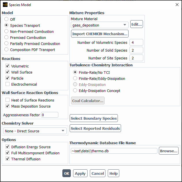
Under Model, select Species Transport.
Under Reactions, select Volumetric.
In the Mixture Material drop-down list under Mixture Properties, select which mixture material you want to use in your problem or, if you want to create your own mixture material, retain the default selection of mixture-template consisting of H2O, O2, and N2. The drop-down list includes all of the mixtures that are currently defined in the database. If there is a mixture material listed that is similar to your desired mixture, you may choose that material and modify it following the steps provided in Defining Properties for the Mixture and Its Constituent Species.
The number of species in the selected mixture material is displayed in the Number of Volumetric Species field and, if applicable, in the Number of Solid Species and Number of Site Species fields. To review the mixture composition and reactions of the selected Fluent database mixture material, click the button to the right of Mixture Material. This opens the Fluent Database Materials dialog box. Clicking, in turn, the View... buttons next to Mixture Species and Reaction opens the corresponding dialog boxes allowing you to examine the constituent species and reactions data. Note, that the mixture properties cannot be edited before the mixture material is copied to your Fluent problem. For this reason, all related controls are dimmed while viewing the mixture properties.
When you enable the species transport model by clicking either or Apply, Ansys Fluent performs the following:
The selected Fluent database mixture material including all constituent fluid materials (species) and properties are automatically copied to your case and appear under Mixture in the tree and the Materials task page.
If any properties for the selected mixture material (or the constituent fluid materials) are missing, the solver prints to the console a notice of the required data.
When the mixture material is copied, the Mixture Material drop-down list in the Species Model dialog box changes to contain only the mixtures defined for your Fluent problem.
The View... button is replaced by the Edit... button giving you an option to access the Edit Material dialog box (Edit Material Dialog Box) from the Species Model dialog box.
The Create/Edit Materials dialog box lists mixture in the Material Type drop-down list allowing you to access the Fluent mixture material database. If you want to check or modify any properties of the mixture material, use the Create/Edit Materials Dialog Box, as described in Defining Properties for the Mixture and Its Constituent Species.
You can add more mixture materials to your case by copying them from the database, as described in Copying Materials from the Ansys Fluent Database, or by creating a new mixture, as described in Creating a New Material and Defining Properties for the Mixture and Its Constituent Species.
Select the Turbulence-Chemistry Interaction (TCI) modeling option. The following options are available:
- Finite-Rate/No TCI
computes only the Arrhenius rate (see Equation 7–21 in the Theory Guide) and neglects turbulence-chemistry interaction. This model is recommended for laminar or turbulent flows using complex chemistry where either the turbulence time-scales are expected to be fast relative to the chemistry time scales or where the chemistry is sufficiently complex that the chemistry timescales of importance are highly disparate throughout the simulation. You can specify the following inputs:
- Flow Iterations per Chemistry Update (steady-state only)
Increasing the number reduces the computational expense of the chemistry calculations. By default, Ansys Fluent will update the chemistry once per flow iteration. This option is not available when the None - Direct Source option is selected for Chemistry Solver.
- Aggressiveness Factor (steady-state only)
This is a numerical factor that controls the robustness and the convergence speed. This value ranges between 0 and 1, where 0 is the most robust, but results in the slowest convergence. The default value for the Aggressiveness Factor is 0.5. This option is available only when Stiff Chemistry Solver or CHEMKIN CFD Solver is selected for Chemistry Solver.
- Temperature Threshold
The reaction rate is highly temperature-dependent. When temperature is low, the reaction rate is fairly small and can be ignored. This may reduce the computational cost without sacrificing accuracy. Ansys Fluent sets the chemistry reaction rate to zero in cells where temperature is below the Temperature Threshold you specified. The default value is 200 K. This option is available only when Stiff Chemistry Solver or CHEMKIN CFD Solver is selected for Chemistry Solver.
- Finite-Rate/Eddy-Dissipation (turbulent flows only)
computes both the Arrhenius rate and the mixing rate and uses the smaller of the two.
- Eddy-Dissipation (turbulent flows only)
computes only the mixing rate (see Equation 7–39 and Equation 7–40 in the Theory Guide).
- Eddy-Dissipation Concept (turbulent flows only)
models turbulence-chemistry interaction with detailed chemical mechanisms (see Equation 7–21 and Equation 7–42 in the Theory Guide). When using this model, you can select the following submodels in the EDC Model group box:
Constant Coefficients (default): Is the standard EDC model described in The Standard EDC Model in the Fluent Theory Guide
Partially Stirred Reactor: Is the partially stirred reactor EDC model described in The Partially Stirred Reactor EDC Model in the Fluent Theory Guide
For both standard and partially stirred reactor EDC models, you can adjust the following parameters:
- Flow Iterations per Chemistry Update (steady-state only)
Increasing the number reduces the computational expense of the chemistry calculations. By default, Ansys Fluent will update the chemistry once per flow iteration.
- Aggressiveness Factor (steady-state only)
This is a numerical factor that controls the robustness and the convergence speed. This value ranges between 0 and 1, where 0 is the most robust, but results in the slowest convergence. The default value for the Aggressiveness Factor is 0.5.
- Temperature Threshold
The reaction rate is highly temperature-dependent. When temperature is low, the reaction rate is fairly small and can be ignored. This may reduce the computational cost without sacrificing accuracy. Ansys Fluent sets the chemistry reaction rate to zero in cells where temperature is below the Temperature Threshold you specified. The default value is 200 K.
For the Constant Coefficients model, you can specify the following parameters:
Volume Fraction Constant: Is
 in Equation 7–44 in the
Theory Guide. The default value is
recommended.
in Equation 7–44 in the
Theory Guide. The default value is
recommended.Time Scale Constant: Is
 in Equation 7–45 in the
Theory Guide. The default value is
recommended.
in Equation 7–45 in the
Theory Guide. The default value is
recommended.
For the Partially Stirred Reactor model, you can select the Mixing Model to compute
 in Equation 7–50 in the Fluent Theory Guide:
Constant Cmix: Sets
 to a constant value specified in Mixing
Constant
to a constant value specified in Mixing
Constant
Dynamic Cmix (default): Computes
 by Equation 7–51 in the Fluent Theory Guide
with the fractal dimension
by Equation 7–51 in the Fluent Theory Guide
with the fractal dimension  in Equation 7–52 in the Fluent Theory Guide
specified in Fractal Dimension
in Equation 7–52 in the Fluent Theory Guide
specified in Fractal Dimension
In addition, you can use your own compiled user-defined functions to calculate EDC scales and to modify the reaction rate as described in
DEFINE_EDC_SCALESandDEFINE_EDC_MDOTin the Fluent Customization Manual.
From the Chemistry Solver drop-down list, select the solver for your simulation (note that the solvers available in the drop-down list are dependent on the selected Turbulence-Chemistry Interaction model):
If you want the stiff chemistry to relax to chemical equilibrium without solving reactions, select Relax to Chemical Equilibrium. This option is not available for Eddy Dissipation Concept. For information about the Relaxation to Chemical Equilibrium model, refer to The Relaxation to Chemical Equilibrium Model in the Theory Guide
Important: The Relax to Chemical Equilibrium chemistry solver requires thermodynamic data of all species to calculate chemical equilibrium. You can supply your own database using the Import CHEMKIN Format Mechanism dialog box (opened by clicking Import CHEMKIN mechanism...) (see Importing a Volumetric Kinetic Mechanism in CHEMKIN Format and Importing a Surface Kinetic Mechanism in CHEMKIN Format for details). A sample database is also contained in the file
.../fluentx.x/cpropep/data/thermo.db. If you define your own species in Ansys Fluent, as determined by the Chemical Formula in the Create/Edit Materials dialog box, and this species name is not in the thermo.db file, Ansys Fluent will report an error. To overcome this error, you must manually enter all the unknown species in the thermo file.If you want to solve finite-rate chemistry, select either Stiff Chemistry Solver or CHEMKIN-CFD Solver. These two solvers are available when using the Finite-Rate/No TCI or Eddy-Dissipation Concept TCI option.
Selecting CHEMKIN-CFD Solver will enable you to use the Ansys CHEMKIN-CFD solution algorithms, which are based on and compatible with the Ansys Chemkin technology. Once you click or , you will be prompted to import a CHEMKIN mechanism, if you have not already done so. Refer to the Ansys Chemkin Input and Theory manuals for details on the chemistry formulation options. See Using Ansys Encrypted Mechanisms for instructions on establishing a CHEMKIN-mechanism based material. In addition, Appendix C: Controlling CHEMKIN-CFD Solver Parameters Using Text Commands includes information about advanced solver settings and diagnostic information for the CHEMKIN-CFD solver. With the Chemkin-CFD Solver selected, the methods for mixture material properties will be defaulted to chemkin. See Procedure for Importing Volumetric CHEMKIN Mechanisms for details.
If you want to make explicit use of chemistry source terms in the species transport equations, without a stiff-chemistry solver, select None - Direct Source. This option is desirable for use with the density-based solver, where the flow and species transport equations are solved monolithically and the explicit use of the chemistry source terms allows the strongest equation coupling. It is however not recommended with the pressure-based solver, where one of the relaxation or stiff-chemistry solvers should be used instead.
(optional) For TCI model options that consider finite-rate chemistry, set the integration parameters using the Integration Parameters dialog box (opened by clicking the button). In the Integration Parameters dialog box, you can the following select acceleration methods (see Using Chemistry Acceleration for more details):
For Stiff Chemistry Solver (single-phase flow): Dynamic Mechanism Reduction (DMR)
See Using Dynamic Mechanism Reduction for details.
For Stiff Chemistry Solver (single-phase flow) or Relax to Chemical Equilibrium: Chemistry Agglomeration (CA)
See Using Chemistry Agglomeration for details.
For any chemistry solver: ISAT
See Using ISAT for details.
For the CHEMKIN-CFD Solver: Dynamic Cell Clustering (DCC) )
See see Using Dynamic Cell Clustering for details.
(optional) Select any Options desired. If you want to model full multicomponent (Stefan-Maxwell) diffusion or thermal (Soret) diffusion, select the Full Multicomponent Diffusion or Thermal Diffusion option, respectively.
See Full Multicomponent Diffusion in the Fluent Theory Guide and Multicomponent Method Inputs for details.
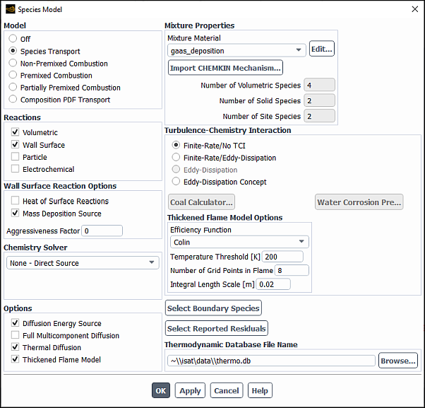
Enable the Thickened Flame Model when modeling unsteady laminar flames, or when using an LES model for turbulent premixed and partially-premixed flames. In the Thickened Flame Model Options group box, specify:
Efficiency Function: Allows you to select one of the following options:
none
Colin (default)
Charlette
When none is selected, then the alteration of the thickening of the flame on its interaction with the turbulence is not considered.
See The Thickened Flame Model in the Fluent Theory Guide for more information about these options.
Number of Grid Points in Flame: Default is 8 grid points.
(simulations with LES only) Integral Length Scale: Is the representative of the largest eddy sizes,
 in Equation 7–57 in the Fluent Theory Guide. You
should provide a value based on the geometry and size of the characteristic bodies (such as
inlet, burners, or bluff bodies). Typically, a value ranging from 1/4 to 1/2 of the
characteristic dimension is used. This item is available only with the
Colin efficiency function.
in Equation 7–57 in the Fluent Theory Guide. You
should provide a value based on the geometry and size of the characteristic bodies (such as
inlet, burners, or bluff bodies). Typically, a value ranging from 1/4 to 1/2 of the
characteristic dimension is used. This item is available only with the
Colin efficiency function.
Consequently, in the Create/Edit Materials dialog box, you will specify the Laminar Flame Speed, for which you have a choice of constant, user-defined, or metghalchi-keck-law, and the Laminar Flame Thickness, for which you have a choice of constant, user-defined, or diffusivity-over-flame-speed.
Note: Since the thickened flame model must capture the correct flame speed, it is imperative that the combination of your chemical mechanism and your molecular transport properties (diffusion coefficients and thermal conductivity) reproduce the correct laminar flame speed. It is recommended that you verify this with a 1D premixed flame simulation using Ansys Chemkin, for example.
When the Thickened Flame Model is enabled (Figure 19.2: The Species Model Dialog Box Displaying the Thickened Flame Model), you have the option to hook a UDF in the User-Defined Function Hooks dialog box to customize the Thickened Flame Model parameters. Refer to
DEFINE_THICKENED_FLAME_MODELin the Fluent Customization Manual for details.Important: The Thickened Flame Model is available only for unsteady laminar or turbulent (LES / DES / SAS / SBES / SDES) flows, with Species Transport and Volumetric Reactions enabled.
For information about the theory behind the Thickened Flame Model, refer to The Thickened Flame Model in the Theory Guide.
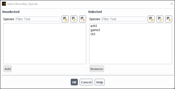
The Species Model Dialog Box(optional) Select the species for which you want to specify boundary conditions. Only the species that you have selected will be listed in the relevant boundary condition dialog boxes. This will facilitate the problem setup, especially when a large number of species are used in a gas mixture. Note that the Patch and Hybrid Initialization dialog boxes, as well as the Solution Initialization task page will also display only the selected species.
Click .
By default, all the gas species for which the transport equations are to be applied are set as boundary species and appear in the Selected multiple-selection list of the Select Boundary Species dialog box (see Figure 19.3: The Select Boundary Species Dialog Box).
Modify the boundary species list as follows:
To remove the species from the Selected Species multiple-selection list, select it and click . The species will be moved from the Selected Species list to the Unselected Species list.
To add the species back to the Selected Species list, simply select it in the Unselected Species multiple-selection list and click . The species will be moved from the Unselected Species list to the Selected Species list.
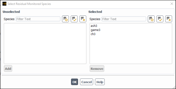
(optional) In a similar manner, click the button and select the species that you want to monitor. Only the residuals for the selected species will be monitored and plotted in the graphics window during the simulation.
By default, all the species for which the species transport equations are to be solved are set as monitored species, and their residual plots will be drawn in the graphics window during the run. For a large number of monitored species, it may be difficult to distinguish the overlapping plot lines. By decreasing the number of monitored species, you can obtain clearer residual plots.
Important:The Fluent solver performs the convergence checks only for the monitored species. To prevent false convergence, make sure to include the species that may have difficulties converging in the monitored species list.
You can modify the list of the monitored species dynamically during a run.
You can import gas kinetics mechanism in CHEMKIN format, which can be used with any solver option. For the CHEMKIN-CFD Solver, native CHEMKIN computations will determine reaction rates, so full compatibility with Ansys Chemkin is provided.
Note: If a mechanism includes at least one reaction type that is not supported in the Fluent material-definition interface (that is, it is not included in the options for manual setup of reactions), the reactions of the CHEMKIN mechanism will not be displayed in the Fluent interface, even though they will be correctly used in Fluent computations.
For information about the format of CHEMKIN volumetric kinetics mechanisms, see Gas-phase Kinetics Input in the Chemkin Input Manual.
For certain types of simulations, Fluent supports the use of encrypted gas kinetics mechanisms, such as those derived from the Ansys Model Fuels Library (encrypted) or through Ansys services. In order to use an encrypted mechanism, you must first import both the gas-phase kinetics and thermodynamic files as described in Procedure for Importing Volumetric CHEMKIN Mechanisms.
When using encrypted CHEMKIN gas mechanisms, note the following points:
Encrypted mechanisms can only be used with the CHEMKIN-CFD solver or the Relax to Chemical Equilibrium option
Prior to importing a flamelet or reading a PDF table generated with an encrypted mechanism, you must first import the mechanism
Chemical equilibrium PDF table generation is not supported
Multiphase and Decoupled Detailed Chemistry models are not supported
You cannot combine encrypted and plain-text gas kinetics, surface kinetics and thermodynamics files in a simulation
The chemistry acceleration options Dynamic Mechanism Reduction (DMR) and Dimension Reduction (DR) are not supported.
Note: The proprietary reaction data will not be displayed in the Fluent interface.
You can import the CHEMKIN mechanism file into Ansys Fluent using the Import CHEMKIN Format Mechanism dialog box (Figure 19.5: The Import CHEMKIN Format Mechanism Dialog Box for Volumetric Kinetics) (opened by clicking in the Species Model dialog box).
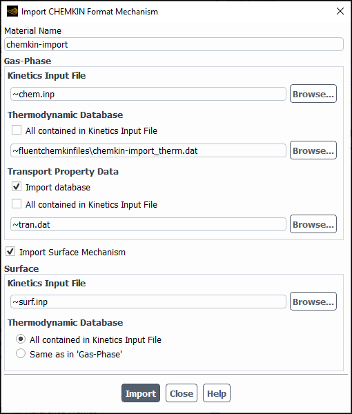
In the Import CHEMKIN Format Mechanism dialog box
Enter a name for the chemical mechanism under Material Name.
Enter the path to the CHEMKIN file (for example,
path/file.inp) in the Kinetics Input File text field in the Gas-Phase group box.
Important:Since Ansys Fluent does not solve for the last species, you must ensure that the last species in the CHEMKIN mechanism species list is an abundant species, such as nitrogen. If not, edit the CHEMKIN mechanism file before importing it into Ansys Fluent, and move the most abundant species (that is the species in your system with the largest total mass fraction) to the end of the species list.
The format for kinetics files is detailed in Chemkin Input Manual. Note that the keyword
ENDmust be added at the end of each group of elements in the input file.The following is an example of a valid format:
ELEMENTSC H NENDSPECIESCH O2 CO2 H2O N2ENDAn example of invalid format is shown below:
ELEMENTSC H NSPECIESCH O2 CO2 H2O N2
Specify species thermodynamic property data. You can include the data in the kinetics input file and/or in a separate file as follows:
If you want to specify thermodynamic data for all species in the kinetics input file, enable All contained in Kinetics Input File to avoid the need to specify a separate file.
If you provide some or all species thermodynamic data in a separate file, disable All contained in Kinetics Input File and specify the thermodynamic data file location.
You can either use the default thermodynamic database file, thermo.db, provided in the cpropep\data directory in your Ansys Fluent installation area or specify the path of your thermodynamic database file if thermo.db does not contain all the gas-phase species in the CHEMKIN mechanism. The format for
thermo.dbis detailed in the CHEMKIN manual [79].Note: Model Fuel Library (MFL) encrypted mechanisms for various fuels have thermodynamic data included in the kinetics input file. See the separate Ansys Model Fuel Library Getting Started Guide for more information about MFL mechanisms.
(optional) To import transport property data, enable Import database under Transport Property Data (Optional) and specify the location of the species transport property data. You can include the data in the kinetics input file and/or in a separate file as follows:
If you want to specify transport property data for all species in the kinetics input file, enable All contained in Kinetics Input File, to avoid the need to specify a separate file.
If you want to provide some or all species transport data in a separate file, disable All contained in Kinetics Input File and specify the transport property data file location.
Ansys Fluent will enable mixture-averaged multicomponent diffusion and set the Lennard-Jones kinetic theory parameters for all the species in the imported CHEMKIN mechanism. If you would like to use Stefan-Maxwell diffusion, enable the Full Multicomponent Diffusion in the Species dialog box.
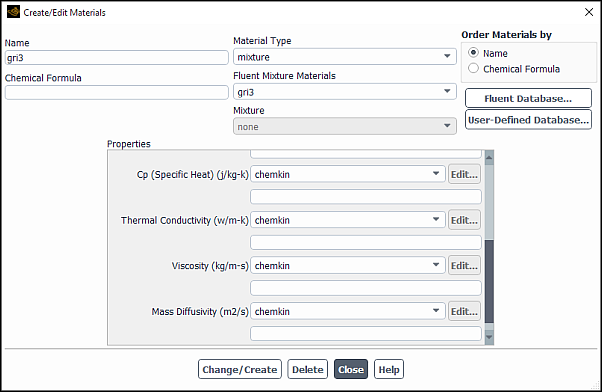
Once the CHEMKIN files are imported, Ansys Fluent creates a material with the specified name, which will contain the data for the species and reactions, and add it to the list of available Mixture Materials in the Create/Edit Materials Dialog Box. The methods to compute the mixture's material properties are set automatically depending on which chemistry solver you selected.
For cases with imported transport property data, the methods used to calculate properties are shown in the table below.
Material Property Stiff Chemistry Solver
CHEMKIN-CFD Solver
Specific Heat
mixing law
chemkin [ a ] Viscosity
ideal-gas-mixing-law
chemkin [ a ] Thermal Conductivity
ideal-gas-mixing-law
chemkin [ a ] Mass Diffusivity
kinetics-theory
chemkin [ a ] Thermal Diffusion
kinetics-theory
chemkin [ a ] For cases with the CHEMKIN-CFD Solver that do not use transport property data, only the Specific Heat mixture property will be automatically set to the chemkin method.
Note that when Full Multicomponent Diffusion is enabled in the Species dialog box, Ansys Chemkin returns full multicomponent diffusivities. If Full Multicomponent Diffusion is disabled, Ansys Chemkin returns mixture averaged mass diffusivities for each species.
Click the button.
Once you click , Ansys Fluent automatically saves the reaction mechanism and thermal files in the data structure. The original input files are not required to be retained along with the Fluent case file. Ansys Fluent will automatically regenerate these files as needed (for example, when using the CHEMKIN-CFD solver).
For information on how to import a surface kinetic mechanism in CHEMKIN format, see Importing a Surface Kinetic Mechanism in CHEMKIN Format.
A CHEMKIN mechanism is a chemical reaction mechanism (also called a chemistry set) that has the following mechanism components:
A file containing thermochemical data for the chemical species of interest
A file containing a description of the reactions occurring in the gas phase
(Optional) A file containing a description of the reactions occurring at the gas-surface interface or on the surface
(Optional) A file containing gas-phase transport data
A set of gas-phase and/or surface reactions are generally developed using specific thermochemical data. Thus, the gas-phase kinetics, surface kinetics, and thermodynamic data are treated as a chemistry “set” in reacting-flow simulations. Ansys Fluent provides the following fuel-combustion mechanisms (including reactions, thermodynamic data, and transport data) that are appropriate for use in common combustion simulations:
Methane / Ethane: 50-species version of GRI-Mech 3.0 (grimech30_50spec)
This is the original GRI-mech 3.0 (53 species) [148] with three species (argon AR, propane C3H8, and propyl radical C3H7) and their reactions removed.
In fuel/air or fuel/oxygen combustion, the removal of these species is expected to have negligible effect on the mechanism predictive capabilities for methane and ethane as fuels. The applicability of the GRI mechanism and validation cases are provided on the GRI mechanism web site [148].
Propane: 37-species high-temperature mechanism (Propane-NOx_highT)
The mechanism has 211 elementary reaction steps and was obtained by removing species and reactions that are unimportant for propane combustion from the comprehensive master mechanism [104]. Ansys Chemkin Reaction Workbench software was used to reduce the master mechanism under the conditions of slightly lean and high pressure laminar flame of a propane/air mixture using the Directed Relation Graph (DRG) method.
Two hydrogen mechanisms:
9-species version for H2 combustion (H2_mech)
The mechanism has 21 elementary reaction steps and has been extracted from Lighthill [88] mechanism for CO and other hydrocarbons.
21-species version for H2 combustion with NOx (H2_NOx_mech)
The mechanism has 105 elementary reaction steps. The hydrogen combustion sub-mechanism is the same as the H2_mech mechanism, above. The NOx sub-mechanism is based on the study by the Glarborg group [127].
As discussed in Overview of User Inputs for Modeling Species Transport and Reactions, if you use a mixture material from the Ansys Fluent database, most mixture and species properties will already be defined. You may follow the procedures in this section to check the current properties, modify some of the properties, or set all properties for a brand-new mixture material that you are defining from nothing.
Remember that you will need to define properties for the mixture material and also for its constituent species. It is important that you define the mixture properties before setting any properties for the constituent species, since the species property inputs may depend on the methods you use to define the properties of the mixture.
The recommended sequence for property inputs is as follows:
Define the mixture species, and reaction(s), and define physical properties for the mixture. Remember to click the button when you are done setting properties for the mixture material.
Define physical properties for the species in the mixture. Remember to click the button after defining the properties for each species.
These steps, all of which are performed in the Create/Edit Materials Dialog Box, are described in detail in this section.
![]() Setup →
Setup → ![]() Materials
Materials
In the Create/Edit Materials dialog box (Figure 19.7: The Create/Edit Materials Dialog Box (Showing a Mixture Material)), check that the Material Type is set to mixture and your mixture is selected in the Fluent Mixture Materials list.
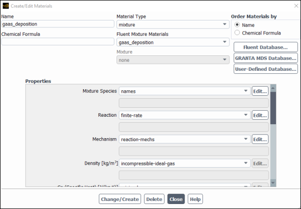
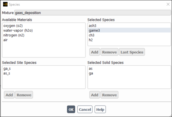
Click the button to the right of Mixture Species under the Properties group box and in the Species Dialog Box (Figure 19.8: The Species Dialog Box) that opens define the species in the mixture material.
Important: For Chemkin mechanisms, the recommended approach for modifying mixture materials is to modify the Chemkin mechanism file and then re-import it into your Fluent case.
In the Species dialog box, the Selected Species list shows all of the fluid-phase species in the mixture. If you are modeling wall or particle surface reactions, the Selected Solid Species list will show all of the bulk solid species in the mixture. Solid species are species that are deposit to, or etch from, wall boundaries or discrete-phase particles (for example, Si(s)) and do not exist as fluid-phase species. If you are modeling wall surface reactions with site balancing, where species adsorb onto the wall surface, react, and then desorb off the surface, the Selected Site Species list will show all of the site species in the mixture.
The use of solid and site species with wall surface reactions is described in Wall Surface Reactions and Chemical Vapor Deposition. See Combusting Particle Surface Reactions for information about particle surface reactions.
Important: The order of the species in the Selected Species list is very important. Ansys Fluent considers the last species in the list to be the bulk species. You should therefore be careful to retain the most abundant species (by mass) as the last species when you add species to or delete species from a mixture material.
The Available Materials list shows materials that are available but not in the mixture. Generally, you will see air in this list, since air is always available by default.
If you are creating a mixture from nothing or starting from an existing mixture and adding some missing species, you will first need to load the desired species from the database (or create them, if they are not present in the database) so that they will be available to the solver. You will need to close the Species dialog box before you begin, since it is a “modal” dialog box that will not allow you to do anything else when it is open. The procedure for adding species is as follows:
In the Create/Edit Materials dialog box, click the button to open the Fluent Database Materials dialog box and copy the desired species, as described in Copying Materials from the Ansys Fluent Database. Remember that the constituent species of the mixture are fluid materials, so you should select fluid as the Material Type in the Fluent Database Materials dialog box to see the correct list of choices. Note that available solid and site species (for surface reactions) are also contained in the fluid list.
Important: If you do not see the species you are looking for in the database, you can create a new fluid material for that species, following the instructions in Creating a New Material, and then continue with step 2, below.
Re-open the Species dialog box. You will see that the fluid materials you copied from the database (or created) are listed in the Available Materials list.
To add a species to the mixture, select it in the Available Materials list and click the button below the Selected Species list (or below the Selected Site Species or Selected Solid Species list, to define a site or solid species). The species will be added to the end of the relevant list and removed from the Available Materials list.
Repeat the previous step for all the desired species. When you are finished, click the button.
Important: Adding a species to the list will alter the order of the species. You should be sure that the last species in the list is the bulk species, and you should check all cell and boundary zone conditions, under-relaxation factors, and other solution parameters that you have set, as described in detail in the following sections.
To remove a species from the mixture, simply select it in the Selected Species list (or the Selected Site Species or Selected Solid Species list) and click the button below the list. The species will be removed from the list and added to the Available Materials list.
Important:
Removing a species from the list will alter the order of the species. You should be sure that the last species in the list is the bulk species, and you should check any cell zone or boundary conditions, under-relaxation factors, or other solution parameters that you have set, as described in detail in the following sections.
Any species that is a reactant, product, or enhanced third-body in an active reaction cannot be deleted from the mixture material.
If you find that the last species in the Selected Species list is not the most abundant species (as it should be), you will need to rearrange the species to obtain the proper order.
Select the bulk species in the Selected Species list.
Click . The selected species will be placed at the end of the Selected Species list. The transport equation of the last species will not be solved.
As discussed previously, you should retain the most abundant species as the last one in the Selected Species list when you add or remove species. Additional considerations you should be aware of when adding and deleting species are presented here.
There are three characteristics of a species that identify it to the solver: name, chemical formula, and position in the list of species in the Species dialog box. Changing these characteristics will have the following effects:
You can change the Name of a species (using the Create/Edit Materials Dialog Box, as described in Renaming an Existing Material) without any consequences.
You should never change the given Chemical Formula of a species.
You will change the order of the species list if you add or remove any species. When this occurs, all cell zone or boundary conditions, solver parameters, and solution data for species will be reset to the default values. (Solution data, cell zone or boundary conditions, and solver parameters for other flow variables will not be affected.) Therefore, if you add or remove species you should take care to redefine species cell zone and boundary conditions and solution parameters for the newly defined problem. In addition, you should recognize that patched species concentrations or concentrations stored in any data file that was based on the original species ordering will be incompatible with the newly defined problem. You can use the data file as a starting guess, but you should be aware that the species concentrations in the data file may provide a poor initial guess for the newly defined model.
If your Ansys Fluent model involves chemical reactions, you can define the reactions in which the defined species participate. This will be necessary only if you are creating a mixture material from nothing, you have modified the species, or you want to redefine the reactions for some other reason.
Depending on which turbulence-chemistry interaction model you selected in the Species Model dialog box (see Enabling Species Transport and Reactions and Choosing the Mixture Material), the appropriate reaction model will be displayed in the Reaction drop-down list in the Edit Material dialog box. If you are using the Finite-Rate/No TCI or Eddy-Dissipation Concept model, the reaction model will be finite-rate; if you are using the Eddy-Dissipation model, the reaction model will be eddy-dissipation; if you are using the Finite-Rate/Eddy-Dissipation model, the reaction model will be finite-rate/eddy-dissipation.
To define the reactions, click the button to the right of Reaction. The Reactions dialog box (Figure 19.9: The Reactions Dialog Box) will open.
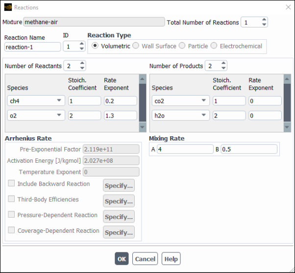
The steps for defining reactions are as follows:
Set the total number of reactions (volumetric reactions, wall surface reactions, and particle surface reactions) in the Total Number of Reactions field. Use the arrows to change the value, or type in the value and press Enter.
Note that if your model includes discrete-phase combusting particles, you should include the particulate surface reaction(s) (for example, char burnout, multiple char oxidation) in the number of reactions only if you plan to use the multiple surface reactions model for surface combustion.
Specify the Reaction Name of the reaction you want to define.
Set the ID of the reaction you want to define. Again, if you type in the value be sure to press Enter.
If this is a fluid-phase reaction, keep the default selection of Volumetric as the Reaction Type. If this is a wall surface reaction (described in Wall Surface Reactions and Chemical Vapor Deposition) or a particle reaction (described in Particle Reactions), select Wall Surface or Particle as the Reaction Type.
Specify how many reactants and products are involved in the reaction by increasing the value of the Number of Reactants and the Number of Products. Select each reactant or product in the Species drop-down list and then set its stoichiometric coefficient and rate exponent in the appropriate Stoich. Coefficient and Rate Exponent fields. The stoichiometric coefficient is the constant
 or
or  in Equation 7–20 in the Theory Guide and
the rate exponent is the exponent on the reactant or product concentration,
in Equation 7–20 in the Theory Guide and
the rate exponent is the exponent on the reactant or product concentration,  or
or  in Equation 7–21 in the Theory Guide.
There are two general classes of reactions that can be handled by the Reactions dialog box, so it is important that the parameters for each reaction are entered correctly. The classes of reactions are as follows:
Global forward reaction (no reverse reaction): Product species generally do not affect the forward rate, so the rate exponent for all products (
 ) should be 0. For reactant species, set the
rate exponent (
) should be 0. For reactant species, set the
rate exponent ( )
to the desired value. If such a reaction is not an elementary reaction,
the rate exponent will generally not be equal to the stoichiometric
coefficient (
)
to the desired value. If such a reaction is not an elementary reaction,
the rate exponent will generally not be equal to the stoichiometric
coefficient ( )
for that species. An example of a global forward reaction is the combustion
of methane:
)
for that species. An example of a global forward reaction is the combustion
of methane:
(19–1)
where
 ,
,  ,
,  ,
,  ,
,  ,
,  ,
,  , and
, and  .
.Figure 19.9: The Reactions Dialog Box shows the coefficient inputs for the combustion of methane. See also the methane-air mixture material in the Fluent Database Materials Dialog Box.
Note that, in certain cases, you may want to model a reaction where product species affect the forward rate. For such cases, set the product rate exponent (
 ) to the desired value. An example of such a reaction is the oxidation of
carbon-monoxide (see the carbon-monoxide-air mixture material in the
Fluent Database Materials Dialog Box), in which the presence of water has
an effect on the reaction rate:
) to the desired value. An example of such a reaction is the oxidation of
carbon-monoxide (see the carbon-monoxide-air mixture material in the
Fluent Database Materials Dialog Box), in which the presence of water has
an effect on the reaction rate:In the gas-shift reaction, the rate expression may be defined as:

(19–2)
where
 ,
,  ,
,  ,
,  ,
,  ,
,  ,
,  , and
, and  .
.Reversible reaction: An elementary chemical reaction that assumes the rate exponent for each species is equivalent to the stoichiometric coefficient for that species. An example of an elementary reaction is the oxidation of SO2 to SO3:
where
 ,
,  ,
,  ,
,  ,
,  ,
and
,
and  .
.See step 7 below for information about how to enable reversible reactions.
If you are using the laminar finite-rate, finite-rate/eddy-dissipation, eddy-dissipation concept or PDF transport model for the turbulence-chemistry interaction, enter the following parameters for the Arrhenius rate in the Arrhenius Rate group box:
Note: All quantities for the Arrhenius rate parameters are in units of kgmol, m3, and seconds.
- Pre-Exponential Factor
(the constant
 in Equation 7–23 in the Theory Guide). The units
of
in Equation 7–23 in the Theory Guide). The units
of  must be specified such that
the units of the molar reaction rate,
must be specified such that
the units of the molar reaction rate,  in Equation 7–19 in the Theory Guide, are moles/volume-time
(for example, kmol/
in Equation 7–19 in the Theory Guide, are moles/volume-time
(for example, kmol/ -s) and the units of the volumetric reaction
rate,
-s) and the units of the volumetric reaction
rate,  in Equation 7–19 in the Theory Guide, are mass/volume-time
(for example, kg/
in Equation 7–19 in the Theory Guide, are mass/volume-time
(for example, kg/ -s).
-s).Important: It is important to note that if you have selected the British units system, the Arrhenius factor should still be entered in SI units. This is because Ansys Fluent applies no conversion factor to your input of
 (the conversion factor is 1.0)
when you work in British units, as the correct conversion factor depends
on your inputs for
(the conversion factor is 1.0)
when you work in British units, as the correct conversion factor depends
on your inputs for  ,
,  ,
and so on.
,
and so on.- Activation Energy
(the constant
 in the forward rate constant
expression, Equation 7–23 in the Theory
Guide).
in the forward rate constant
expression, Equation 7–23 in the Theory
Guide).- Temperature Exponent
(the value for the constant
 in Equation 7–23 in the Theory Guide).
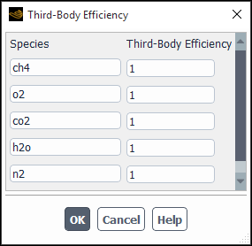
- Third-Body Efficiencies
(the values for
 in Equation 7–22 in the Theory Guide). If you
have accurate data for the efficiencies and want to include this effect
on the reaction rate (that is, include
in Equation 7–22 in the Theory Guide). If you
have accurate data for the efficiencies and want to include this effect
on the reaction rate (that is, include  in Equation 7–21 in the Theory Guide), select
the Third Body Efficiencies option and click
the button to open the Third-Body Efficiency Dialog Box (Figure 19.10: The Third-Body Efficiency Dialog Box).
in Equation 7–21 in the Theory Guide), select
the Third Body Efficiencies option and click
the button to open the Third-Body Efficiency Dialog Box (Figure 19.10: The Third-Body Efficiency Dialog Box).For each Species in the dialog box, specify the Third-Body Efficiency.
Important: It is not necessary to include the third-body efficiencies. You should not enable the Third-Body Efficiencies option unless you have accurate data for these parameters.
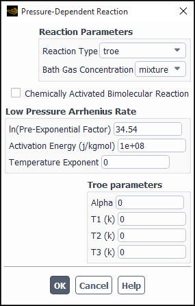
- Pressure-Dependent Reaction
(if relevant) If you are using the laminar finite-rate or eddy-dissipation concept model for turbulence-chemistry interaction, or have selected the composition PDF transport model (see Modeling a Composition PDF Transport Problem), and the reaction is a pressure fall-off reaction (see Pressure-Dependent Reactions in the Theory Guide), enable the Pressure-Dependent Reaction option for the Arrhenius Rate and click the button to open the Pressure-Dependent Reaction dialog box (Figure 19.11: The Pressure-Dependent Reaction Dialog Box).
Under Reaction Parameters, select the appropriate Reaction Type (lindemann, troe, or sri). See Pressure-Dependent Reactions in the Theory Guide for details about the three methods. Next, specify if the Bath Gas Concentration (
 in Equation 7–32 in the Theory Guide) is to
be defined as the concentration of the mixture, or as the concentration of one of the mixture’s constituent
species, by selecting the appropriate item in the drop-down list.
in Equation 7–32 in the Theory Guide) is to
be defined as the concentration of the mixture, or as the concentration of one of the mixture’s constituent
species, by selecting the appropriate item in the drop-down list.Enabling the Chemically Activated Bimolecular Reaction option results in a net rate constant at any pressure being defined as Equation 7–38 in the Theory Guide.
The parameters you specified under Arrhenius Rate in the Reactions dialog box represent the high-pressure Arrhenius parameters. You can, however, specify values for the following parameters under Low Pressure Arrhenius Rate:
- ln(Pre-Exponential Factor)
(
 in Equation 7–30 in the Theory Guide) The pre-exponential
factor
in Equation 7–30 in the Theory Guide) The pre-exponential
factor  is
often an extremely large number, so you will input the natural logarithm
of this term.
is
often an extremely large number, so you will input the natural logarithm
of this term.- Activation Energy
(
 in Equation 7–30 in
the Theory Guide)
in Equation 7–30 in
the Theory Guide)- Temperature Exponent
(
 in Equation 7–30 in the Theory Guide)
If you selected troe for the Reaction Type, you can specify values for Alpha, T1, T2, and T3 (
 ,
,  ,
,  , and
, and  in Equation 7–35 in the Theory Guide) under Troe parameters. If you selected sri for the Reaction Type, you can specify values
for a, b, c, d, and e (
in Equation 7–35 in the Theory Guide) under Troe parameters. If you selected sri for the Reaction Type, you can specify values
for a, b, c, d, and e ( ,
,  ,
,  ,
,  , and
, and  in Equation 7–36 in the Theory Guide) under SRI parameters.
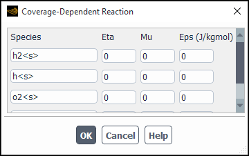
- Coverage Dependent Reaction
If you are modeling Wall Surface reactions with site-balancing and you have reaction rates that depend on site coverages, you can enable the Coverage Dependent Reaction option. Click to open the Coverage Dependent Reaction dialog box (Figure 19.12: The Coverage Dependent Reaction Dialog Box) and input the coverage parameters.
In the Coverage Dependent Reaction dialog box, all the site species of the reaction will be present with a default value of 0 for all the parameters, corresponding to no surface coverage modification. Enter the relevant values of the parameters
 ,
,  , and
, and  (as defined in Equation 7–81 in the Theory Guide) for all the species for which the reaction has coverage dependence.
  and
and  are dimensionless,
and
are dimensionless,
and  is in units of J/kgmol.
If you are using the laminar finite-rate, eddy-dissipation concept or PDF transport model for turbulence-chemistry interaction, and the reaction is reversible, enable the Include Backward Reaction option for the Arrhenius Rate. When this option is enabled, you will not be able to edit the Rate Exponent for the product species, which instead will be set to be equivalent to the corresponding product Stoich. Coefficient. By default, Ansys Fluent calculates the reverse reaction rate constants using Equation 7–24 in the Fluent Theory Guide. You can overwrite the Ansys Fluent’s default parameters for the reactions or define your own reactions. In both scenarios, you also need to specify the standard-state enthalpy and standard-state entropy for mixture material. Ansys Fluent will use these values in the calculation of the backward reaction rate constant (Equation 7–24 in the Fluent Theory Guide).
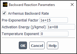
In addition, you have the option to provide your own backward reaction parameters. To do this, click Specify... next to Include Backward Reaction and enable the Arrhenius Backward Rate option in the Backward Reaction Parameters dialog box that opens (see Figure 19.13: Backward Reaction Parameters Dialog Box).
You can specify the following backward rate parameters:
- Pre-Exponential Factor
(the constant
 in Equation 7–28 in the Fluent Theory Guide).
 - Activation Energy
(the constant
 in the backward rate
constant expression in Equation 7–28 in the Fluent Theory Guide).
in the backward rate
constant expression in Equation 7–28 in the Fluent Theory Guide).- Temperature Exponent
(the constant
 in Equation 7–28 in the Fluent Theory Guide).
Ansys Fluent will use your custom values to calculate the backward rate constant of the reversible reaction according to Equation 7–28 in the Fluent Theory Guide.
Note that the reversible reaction option is not available for either the eddy-dissipation or the finite-rate/eddy-dissipation turbulence-chemistry interaction model.
If you are using the eddy-dissipation or finite-rate/eddy-dissipation model for turbulence-chemistry interaction, you can enter values for A and B under the Mixing Rate heading. These values should not be changed unless you have reliable data. In most cases you will use the default values.
A is the constant
 in the turbulent mixing rate
(Equation 7–39 and Equation 7–40 in the Theory Guide) when it
is applied to a species that appears as a reactant in this reaction.
The default setting of 4.0 is based on the empirically derived values
given by Magnussen et al. [94].
in the turbulent mixing rate
(Equation 7–39 and Equation 7–40 in the Theory Guide) when it
is applied to a species that appears as a reactant in this reaction.
The default setting of 4.0 is based on the empirically derived values
given by Magnussen et al. [94].B is the constant
 in the turbulent mixing rate
(Equation 7–40 in
the Theory Guide) when it is applied to a species that appears as a product in this
reaction. The default setting of 0.5 is based on the empirically derived
values given by Magnussen et al. [94].
in the turbulent mixing rate
(Equation 7–40 in
the Theory Guide) when it is applied to a species that appears as a product in this
reaction. The default setting of 0.5 is based on the empirically derived
values given by Magnussen et al. [94].Repeat steps 2–8 for each reaction you need to define. After defining all reactions, click .


Quite often, combustion systems will include fuel that is not easily described as a pure
species (such as CH4 or
C2H6). Complex hydrocarbons, including fuel oil
or even wood chips, may be difficult to define in terms of such pure species. However, if you
have available the heating value and the ultimate analysis (elemental composition) of the
fuel, you can define an equivalent fuel species and an equivalent heat of formation for this
fuel. Consider, for example, a fuel known to contain 50% C, 6% H, and 44% O by weight.
Dividing by atomic weights, you can arrive at a “fuel” species with the
molecular formula
C4.17H6O275. You can
start from a similar, existing species or create a species from nothing, and assign it a
molecular weight of 100.04 kg/kmol (4.17  12 + 6
  1 + 2.75
  16). The chemical reaction would be considered to be
 | (19–3) |
You will need to set the appropriate stoichiometric coefficients for this reaction.
The heat of formation (or standard-state enthalpy) for the fuel
species can be calculated from the known heating value  since
since
 | (19–4) |
where  is the standard-state
enthalpy on a molar basis. Note the sign convention in Equation 19–4 :
is the standard-state
enthalpy on a molar basis. Note the sign convention in Equation 19–4 :  is negative
when the reaction is exothermic.
is negative
when the reaction is exothermic.
If your Ansys Fluent model involves reactions that are confined to a specific area of the domain, you can define “reaction mechanisms” to enable different reactions selectively in different geometrical zones. You can create reaction mechanisms by selecting reactions from those defined in the Reactions dialog box and grouping them. You can then assign a particular mechanism to a particular zone.
To define a reaction mechanism, click the button to the right of Mechanism. The Reaction Mechanisms Dialog Box (Figure 19.14: The Reaction Mechanisms Dialog Box) will open.
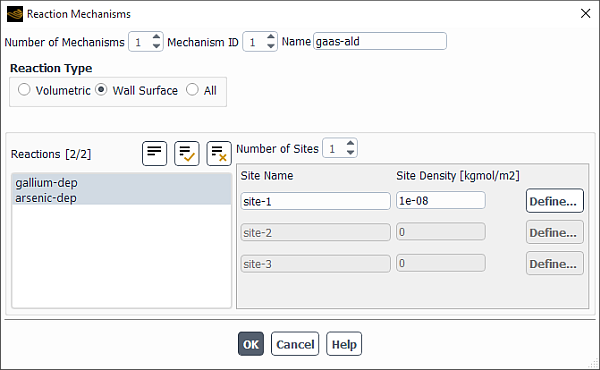
The steps for defining a reaction mechanism are as follows:
Set the total number of mechanisms in the Number of Mechanisms field. Use the arrows to change the value, or type the value and press Enter.
Set the Mechanism ID of the mechanism you want to define. Again, if you type in the value, be sure to press Enter.
Specify the Name of the mechanism.
Select the type of reaction to add to the mechanism under Reaction Type. If you select Volumetric, the Reactions list will display all available fluid-phase reactions. If you select Wall Surface or Particle, the Reactions list will display all available wall surface reactions (described in Wall Surface Reactions and Chemical Vapor Deposition) or particle reactions (described in Particle Reactions). If you select All, the Reactions list will display all available reactions. This option is meant for backward compatibility with Ansys Fluent 6.0 or earlier cases.
Select the reactions to be included in the mechanism.
For Volumetric or Particle reactions, select available reactions for the mechanism in the Reactions list.
For Wall Surface reactions, use the following procedure:
Select available wall surface reactions for the mechanism in the Reactions list.
If any site species appear in the selected reaction(s), set the number of sites in the Number of Sites field. Use the arrows to change the value, or type the value and press Enter. See Reaction-Diffusion Balance for Surface Chemistry in the Theory Guide for details about site species in wall surface reactions.
If you specify a Number of Sites that is greater than zero, specify the properties of the site.
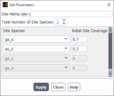
Click the button. This will open the Site Parameters Dialog Box (Figure 19.15: The Site Parameters Dialog Box), where you will define the parameters of the site species.
- Site Name
is the optional name of the site that was specified in the Reaction Mechanisms dialog box.
- Total Number of Site Species
is the number of adsorbed species that are to be modeled at the site. (Use the arrows to change the value, or type the value and press Enter.)
Under Site Species, select the appropriate species from the drop-down list(s) and specify the fractional Initial Site Coverage for each species. For steady-state calculations, it is recommended (though not strictly required) that the initial values of Initial Site Coverage sum to unity. For transient calculations, it is required that these values sum to unity.
Click in the Site Parameters dialog box to store the new values.
Repeat steps 2–5 for each reaction mechanism you need to define. When you are finished defining all reaction mechanisms, click .
When your Ansys Fluent model includes chemical species, the following physical properties must be defined, either by you or by the database, for the mixture material:
density, which you can define using the gas law or as a volume-weighted function of composition
viscosity, which you can define as a function of composition
thermal conductivity and specific heat (in problems involving solution of the energy equation), which you can define as functions of composition
mass diffusion coefficients and Schmidt number, which govern the mass diffusion fluxes (Equation 7–2 and Equation 7–4 in the Theory Guide)
Detailed descriptions of these property inputs are provided in Physical Properties.
Important: Remember to click the button when you are done setting the properties of the mixture material. The properties that appear for each of the constituent species will depend on your settings for the properties of the mixture material. If, for example, you specify a composition-dependent viscosity for the mixture, you will need to define viscosity for each species.
For each of the fluid materials in the mixture, you (or the database) must define the following physical properties:
molecular weight, which is used in the gas law and/or in the calculation of reaction rates and mole-fraction inputs or outputs
standard-state (formation) enthalpy and reference temperature (in problems involving solution of the energy equation)
viscosity, if you defined the viscosity of the mixture material as a function of composition
thermal conductivity and specific heat (in problems involving solution of the energy equation), if you defined these properties of the mixture material as functions of composition
standard-state entropy, if you are modeling reversible reactions
thermal and momentum accommodation coefficients, if you have enabled the low-pressure boundary slip model.
Detailed descriptions of these property inputs are provided in Physical Properties.
Important: Global reaction mechanisms with one or two steps inevitably neglect the intermediate species. In high-temperature flames, neglecting these dissociated species may cause the temperature to be overpredicted. A more realistic temperature field can be obtained by increasing the specific heat capacity for each species. Rose and Cooper [130] have created a set of specific heat polynomials as a function of temperature.
The specific heat capacity for each species is calculated as
 | (19–5) |
The modified  polynomial coefficients (J/kg-K) are provided in Table 19.1: Modified Specific Heat Capacity (Cp) Polynomial Coefficients .
Table 19.1: Modified Specific Heat Capacity (Cp) Polynomial Coefficients
| Coefficient |

|

|

|
|---|---|---|---|

| 5.35446e+02 | 1.93780e+03 | 8.76317e+02 |

| 1.27867e+00 | -1.18077e+00 | 1.22828e-01 |

| -5.46776e-04 | 3.64357e-03 | 5.58304e-04 |

| -2.38224e-07 | -2.86327e-06 | -1.20247e-06 |

| 1.89204e-10 | 7.59578e-10 | 1.14741e-09 |

| — | — | -5.12377e-13 |

| — | — | 8.56597e-17 |
The Coal Calculator dialog box automates calculation and setting of the relevant input parameters for the Species, Discrete-Phase (DPM) and Pollutant models associated with coal combustion. It is available in the Species dialog box for the Species Transport model when the Eddy-Dissipation or Finite-Rate/Eddy-Dissipation turbulence-chemistry option is selected. You can define up to three coal streams in your simulation using the Number of Coal Streams entry box.
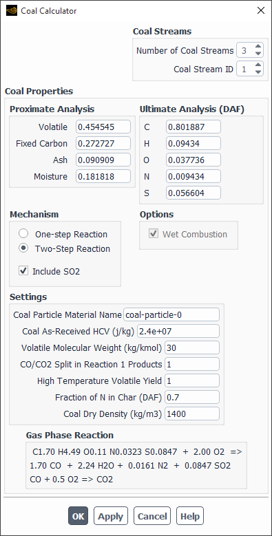
For each coal stream selected in the Coal Stream ID, you need to define the following properties:
Coal Proximate Analysis, which is the mass fraction of Volatile, Fixed Carbon, Ash and Moisture in the coal. Ansys Fluent will normalize the mass fractions so that they sum to unity.
Coal Ultimate Analysis, which is the mass fraction of atomic C, H, O, N and optionally S, in the Dry-Ash-Free (DAF) coal. Ansys Fluent will normalize the mass fractions so that they sum to unity.
A choice of One-step or Two-step chemical mechanism. The one-step mechanism is,

(19–6)
The two-step mechanism involves oxidation of volatiles to CO in the first reaction and oxidation of CO to CO2 in the second reaction:

(19–7)
The stoichiometric coefficients in Equation 19–6 and Equation 19–7 are calculated from the ultimate and proximate analyses.
An option to Include SO2. When this is enabled, an input for the atomic mass fraction of sulphur, S, appears in the ultimate analysis frame.
The Coal Particle Material Name. A DPM combusting-particle material will be created with this name. The default name is coal-particle.
The Coal As-Received HCV, where HCV denotes the Higher Calorific Value.
Volatile Molecular Weight is the molecular weight of pure volatiles.
The CO/CO2 Split in Reaction 1 Products can be used to specify the molar fraction of CO to CO2 in the first reaction of Equation 19–7. The default value of 1 implies that all carbon is reacted to CO, with no CO2 produced.
The High Temperature Volatile Yield. Enhanced devolatization at higher temperatures can cause the volatile yield to exceed the proximate analysis fraction. To model this, the actual volatile fraction used is calculated as that specified in the Proximate Analysis input multiplied by the High Temperature Volatile Yield. The actual fixed carbon fraction is then calculated as one minus the sum of the actual volatile, ash and moisture fractions.
Fraction of N in Char (DAF). This input is used in calculating the split of atomic nitrogen for the Fuel NOx model.
Coal Dry Density is used to calculate the volume fraction of liquid-water for the Wet Combustion option in the Injections dialog box.
Clicking Apply will save the Coal Property data for the selected Coal Stream ID. When you click , Ansys Fluent makes the following changes:
A Mixture material is created, named coal-volatiles-air, with a one or two step reaction mechanism as specified in the Mechanism option. If the Fluid material species (O2, CO, CO2, and so on) do not exist, they are created. A Fluid material called coal-volatiles, is also created with a standard state enthalpy calculated from the ultimate and proximate analyses, as-received HCV and volatile molecular weight. For the second and third coal streams, additional Fluid materials and reactions with the properties corresponding to the second and third coal streams are also created in the mixture.
A combusting-particle material is created for each coal stream with Volatile Component Fraction and Combustible Fraction calculated from the ultimate and proximate analyses. The discrete phase model (DPM) is enabled.
For the fuel NOx model, the default fuel species is set to vol, the char N conversion is set to NO, and the fuel NOx Volatile and Char mass fractions are set according to the ultimate and proximate compositions of the first coal stream. Note that even though some of the default fuel NOx parameters are changed, the fuel NOx model itself is not enabled.
If the Moisture mass fraction in the coal proximate analysis is nonzero, then the Wet Combustion option is enabled in the Coal Calculator dialog box, and all subsequent injections that are created will have wet combustion enabled. The liquid material will be set to
water-liquid, and the volume fraction of water will be calculated from the Moisture mass fraction specified in the proximate analysis and the Coal Dry Density. The wet combustion settings are not modified for existing injections. The Density for the combusting-particle in the Create/Edit Materials dialog box will also be set to Coal Dry Density.
Note: Irrespective of the Wet Combustion option in the Coal Calculator dialog box you can modify the Wet Combustion model setting for the injections in the Set Injection Properties dialog box. In addition, you will need to take care to enter the flow-rate of each injection on a wet or dry basis, consistent with the Wet Combustion model setting.
You will need to specify the inlet mass fraction for all species in your simulation. In addition, for pressure outlets you will set species mass fractions to be used in case of backflow. At walls, Ansys Fluent will apply a zero-gradient (zero-flux) boundary condition for all species by default, although you can change each species boundary condition to a specified value. If you have surface reactions defined (see Wall Surface Reactions and Chemical Vapor Deposition), you can choose to enable wall-surface reactions and select the chemical mechanism. For fluid zones, you also have the option of specifying a reaction mechanism. Input of cell zone and boundary conditions is described in Cell Zone and Boundary Conditions.
Note: In a single-phase case with all fluid zones, only one mixture material can be assigned to the zones. However, if the fluid zones are separated by walls, then one mixture and any number of non-mixture (pure fluid) materials can be assigned to different zones.
Important:
Non-reflecting boundary conditions (NRBCs) are not compatible with species transport models. They are mainly used to solve ideal-gas single species flow. For information about NRBCs, see Boundary Acoustic Wave Models.
Note that you will explicitly set mass fractions only for the first
 species. The solver will
compute the mass fraction of the last species by subtracting the total
of the specified mass fractions from 1. If you want to explicitly
specify the mass fraction of the last species, you must reorder the
species in the list (in the Create/Edit Materials Dialog Box), as described in Defining Properties for the Mixture and Its Constituent Species.
species. The solver will
compute the mass fraction of the last species by subtracting the total
of the specified mass fractions from 1. If you want to explicitly
specify the mass fraction of the last species, you must reorder the
species in the list (in the Create/Edit Materials Dialog Box), as described in Defining Properties for the Mixture and Its Constituent Species.
For the pressure-based solver in Ansys Fluent, the net transport of species at inlets consists of
both convection and diffusion components. The convection component is fixed by the specified
inlet species mass or mole fraction, whereas the diffusion component depends on the gradient of
the computed species concentration field (which is not known a priori). At very small
convective inlet velocities, for example when modeling perforated combustion liners with an
inlet, substantial mass can be gained or lost through the inlet due to diffusion. For this
reason, inlet diffusion is disabled by default, but can be enabled with the
define/models/species/inlet-diffusion text command.
You can define a source or sink of a chemical species within the computational domain by defining a source term in the Fluid dialog box. You may choose this approach when species sources exist in your problem but you do not want to model them through the mechanism of chemical reactions. Defining Mass, Momentum, Energy, and Other Sources describes the procedures you would follow to define species sources in your Ansys Fluent model. If the source is not a constant, you can use a user-defined function. See the Fluent Customization Manual for details about user-defined functions.
While many simulations involving chemical species may require no special procedures during the solution process, you may find that one or more of the solution techniques noted in this section helps to accelerate the convergence or improve the stability of more complex simulations. The techniques outlined below may be of particular importance if your problem involves many species and/or chemical reactions, especially when modeling combusting flows.
Obtaining a converged solution in a reacting flow can be difficult for a number of reasons. First, the impact of the chemical reaction on the basic flow pattern may be strong, leading to a model in which there is strong coupling between the mass/momentum balances and the species transport equations. This is especially true in combustion , where the reactions lead to a large heat release and subsequent density changes and large accelerations in the flow. All reacting systems have some degree of coupling, however, when the flow properties depend on the species concentrations. These coupling issues are best addressed by the use of a two-step solution process, as described below, and by the use of under-relaxation as described in Setting Under-Relaxation Factors.
A second convergence issue in reacting flows involves the magnitude of the reaction source term. When the Ansys Fluent model involves very rapid reaction rates (reaction time scales are much faster than convection and diffusion time scales), the solution of the species transport equations becomes numerically difficult. Such systems are termed “stiff” systems. Stiff systems with finite-rate chemistry should be solved using either the pressure-based or density-based solver together with either Stiff Chemistry Solver or the CHEMKIN-CFD Solver (see Solution of Stiff Chemistry Systems). Finite-rate chemistry may also be used for turbulent combustion. For turbulent combustion, turbulence-chemistry interactions can either be neglected (Finite-rate/No TCI model) or accounted for using Eddy-Dissipation Concept or PDF Transport models.
Solving a reacting flow as a two-step process is a practical method for reaching a stable converged solution to your Ansys Fluent problem. In this process, you begin by solving the flow, energy, and species equations with reactions disabled (the “cold-flow”, or unreacting flow). When the basic flow pattern has thereby been established, you can re-enable the reactions and continue the calculation. The cold-flow solution provides a good starting solution for the calculation of the combusting system. This two-step approach to combustion modeling can be accomplished using the following procedure:
Set up the problem including all species and reactions of interest.
Temporarily disable reaction calculations by turning off Volumetric in the Species Model Dialog Box.
 Setup → Models → Species
  Edit...
Disable calculation of the product species in the Equations Dialog Box.
Solution →  Controls
→ Equations...
Controls
→ Equations...
Calculate an initial (cold-flow) solution. (Note that it is generally not productive to obtain a fully converged cold-flow solution unless the non-reacting solution is also of interest to you.)
Enable the reaction calculations by turning on Volumetric again in the Species Model Dialog Box.
Enable all equations in the Equations dialog box. If you are using the Finite-Rate/No TCI, Finite-Rate/Eddy-Dissipation, Eddy-Dissipation Concept or PDF Transport model for the turbulence-chemistry interaction, you may need to patch an ignition source (as described in Ignition in Steady-State Combustion Simulations).
One of the main reasons a combustion calculation can have difficulty converging is that large changes in temperature cause large changes in density, which can, in turn, cause instabilities in the flow solution. When you use the pressure-based solver, Ansys Fluent allows you to under-relax the change in density to alleviate this difficulty. The default value for density under-relaxation is 1, but if you encounter convergence trouble you may want to reduce this to a value between 0.5 and 1 (in the Solution Controls task page).
Note that if you are using a real-gas model the solution might converge at a slower rate than when running ideal-gas flow. To improve the convergence performance of your analysis, you need to reduce the underrelaxation for density to values as low as 0.1.
If you introduce fuel to an oxidant or have a premixed fuel/oxidant mixture, but you are not simulating the transient ignition process, then you must numerically force the solution to the burned state (rather than the unburned state). Generally, spontaneous ignition does not occur unless the temperature of the mixture exceeds the activation energy threshold required to maintain combustion. For steady-state Ansys Fluent combustion simulations, whether you are using the species transport or PDF transport model and regardless of turbulence-chemistry interaction option, you have to supply an ignition source to initiate combustion. This ignition source may be a heated surface or inlet mass flow that heats the gas mixture above the required ignition temperature. Often, however, it is the equivalent of a spark: an initial solution state that causes combustion to proceed. You can supply this initial “spark” by patching a hot temperature into a region of the Ansys Fluent model that contains an ignitable fuel/air mixture.
![]() Solution →
Solution → ![]() Initialization → Patch...
Initialization → Patch...
Depending on the model, you may need to patch both the temperature and the fuel/ oxidant/product concentrations to produce ignition in your model. The initial patch has no impact on the final steady-state solution—no more than the location of a match determines the final flow pattern of the torch that it lights. See Patching Values in Selected Cells for details about patching initial values.
When modeling stiff chemistry systems, such as flames with finite-rate kinetics, you can either use the pressure-based solver with the Stiff Chemistry Solver option enabled or CHEMKIN-CFD Solver selected as seen in the Species Model Dialog Box (Figure 19.1: The Species Model Dialog Box), or the density-based solver.
For steady simulations using the pressure-based solver, the Stiff Chemistry Solver option approximates the reaction
rate  in the species transport equation
(see Equation 7–19 in the Theory Guide) as,
in the species transport equation
(see Equation 7–19 in the Theory Guide) as,
 | (19–8) |
where  is an appropriate time step size. Note that as
  tends to zero the approximation becomes exact but the stiff numerics will
cause the pressure-based solver to diverge. On the other hand, as
tends to zero the approximation becomes exact but the stiff numerics will
cause the pressure-based solver to diverge. On the other hand, as  tends to infinity, the approximated reaction rate
  tends to zero and, while the numerical stiffness is alleviated, there is no
reaction. In Ansys Fluent, the default value for
tends to zero and, while the numerical stiffness is alleviated, there is no
reaction. In Ansys Fluent, the default value for  is set to one-tenth of the minimum convective or diffusive time-scale in the
cell. This value was found to be sufficiently accurate and robust, although it can be modified
using the
is set to one-tenth of the minimum convective or diffusive time-scale in the
cell. This value was found to be sufficiently accurate and robust, although it can be modified
using the solve/set/stiff-chemistry text command. ISAT is employed to
integrate the stiff chemistry in Equation 19–8. Equation 19–8 is also applied for unsteady simulations, with
 = flow time step size.
Details about the ISAT algorithm may be found in Particle Reaction in the Theory Guide and Using ISAT Efficiently. For efficient and accurate use of ISAT, a review of this section is highly recommended.
The density-based implicit solver may also be used with either chemistry solver option. This option allows a larger stable Courant (CFL) number specification, although additional calculations are required to calculate the eigenvalues of the chemical system Jacobian [170]. When enabling the stiff-chemistry solver with the density-based solver, the following must be specified:
Temperature Positivity Rate Limit: limits new temperature changes by this factor multiplied by the old temperature. Its default value is 0.2.
Temperature Time Step Reduction: limits the local CFL number when the temperature is changing too rapidly. Its default value is 0.25.
The Eddy Dissipation Concept (EDC) model is used to consider detailed chemistry and its interaction with turbulence. Due to the use of an ODE solver to obtain the fine scale species mass fractions and temperature, the computational expense of the EDC model can be high. One efficient solution procedure is to first use the relaxation to chemical equilibrium model (see The Relaxation to Chemical Equilibrium Model in the Fluent Theory Guide) to quickly obtain an initial solution and then switch to the EDC model to complete the runs for the desired accuracy.
Note that the default numerical parameters for the solution of the EDC equations are set to provide maximum robustness with slowest convergence. The convergence rate can be increased by setting the Aggressiveness Factor in the Species dialog box or with the text command:
define → models →
species →
set-turb-chem-interaction
The Aggressiveness Factor can be set from 0 (slow but stable) to 1 (fast but least stable). The default is 0.5.
Ansys Fluent can report chemical species as mass fractions, mole fractions, and molar concentrations. You can also display laminar and effective mass diffusion coefficients. The following variables are available for postprocessing of species transport and reaction simulations:
Mass fraction of species-n
Mole fraction of species-n
Molar Concentration of species-n
Lam Diff Coef of species-n
Eff Diff Coef of species-n
Thermal Diff Coef of species-n
Enthalpy of species-n (pressure-based solver calculations only)
species-n Source Term (density-based solver calculations only)
Relative Humidity
TFM Thickening Factor (Thickened Flame Model only)
TFM Omega (Thickened Flame Model only)
TFM Thickening Factor (turbulent cases (LES / DES / SAS / SBES / SDES) with Thickened Flame Model only)
Laminar Flame Speed (Thickened Flame Model only)
Laminar Flame Thickness (Thickened Flame Model only)
Cell Time Scale (Eddy-Dissipation Concept and laminar finite-rate with stiff-chemistry only)
Fine Scale Mass fraction of species-n (Eddy-Dissipation Concept model only)
EDC Cell Volume Fraction (Eddy-Dissipation Concept model only)
Fine Scale Temperature (Eddy-Dissipation Concept model only)
Net Rate of species-n (Eddy-Dissipation Concept and laminar finite-rate with stiff-chemistry only)
Kinetic Rate of Reaction-n
Turbulent Rate of Reaction-n
Liquid species mass fraction of species-n (solidification and melting model only)
Heat of Reaction
These variables are contained in the Species..., Temperature..., and Reactions... categories of the variable selection drop-down list that appears in postprocessing dialog boxes. See Field Function Definitions for a complete list of flow variables, field functions, and their definitions. Displaying Graphics and Reporting Alphanumeric Data explain how to generate graphics displays and reports of data.
Note: The net reaction rates of species are computed during the solution of transport equations, and, therefore, you need to run at least one iteration to obtain correct values for postprocessing.
Averaged species concentrations at inlets and exits, and across selected planes (that is, surfaces that you have created using Create in the Domain ribbon tab (Surfacegroup box)) within your model can be obtained using the Surface Integrals Dialog Box, as described in Surface Integration.
![]() Results → Reports → Surface Integrals
Results → Reports → Surface Integrals ![]() Edit...
Edit...
Select the Molar Concentration of species-n for the appropriate species in the Field Variable drop-down list.
For gas-phase reactions, the reaction rate is defined on a volumetric basis and the rate of creation and destruction of chemical species becomes a source term in the species conservation equations. Heterogeneous surface reactions create sources (and sinks) of chemical species in the gas-phase as well, but also alter surface coverages for surface site reactions, and may deposit or etch species for bulk (solid) reactions.
For more information about the theoretical background of wall surface reactions and chemical vapor depositions, see Wall Surface Reactions and Chemical Vapor Deposition in the Theory Guide. Information about using wall surface reactions is presented in the following subsections:
- 19.1.2.1. Overview of Surface Species and Wall Surface Reactions
- 19.1.2.2. Importing a Surface Kinetic Mechanism in CHEMKIN Format
- 19.1.2.3. Manual Inputs for Wall Surface Reactions
- 19.1.2.4. Including Mass Transfer To Surfaces in the Continuity Equation
- 19.1.2.5. Wall Surface Mass Transfer Effects in the Energy Equation
- 19.1.2.6. Modeling the Heat Release Due to Wall Surface Reactions
- 19.1.2.7. Solution Procedures for Wall Surface Reactions
- 19.1.2.8. Postprocessing for Surface Reactions
Ansys Fluent treats chemical species adsorbed and desorbed, as well as those deposited into or etched from the bulk solid surfaces as distinct from the same chemical species in the gas. Similarly, surface reactions are defined distinctly and treated differently than gas-phase reactions involving the same chemical species.
Surface reactions can be limited so that they occur on only some of the wall boundaries (while the other wall boundaries remain free of surface reaction). The surface reaction rate is defined and computed per unit surface area, in contrast to the fluid-phase reactions, which are based on unit volume.
Importing surface kinetic mechanisms in CHEMKIN format requires that the gas-phase mechanism file accompanies the surface mechanism file for full compatibility with CHEMKIN (for more information on how to import the gas-phase mechanism, see Importing a Volumetric Kinetic Mechanism in CHEMKIN Format). If the gas-phase mechanism file is not available, then you will need to create one that you will import along with the surface mechanism file. For information about the format of CHEMKIN surface kinetics mechanisms, see Surface Kinetics Input in the Chemkin Input Manual.
The mechanism files are imported into Ansys Fluent using the Import CHEMKIN Format Mechanism dialog box (Figure 19.17: The Import CHEMKIN Format Mechanism Dialog Box for Surface Kinetics) which is opened by clicking Import CHEMKIN Mechanism... in the Species Model dialog box.
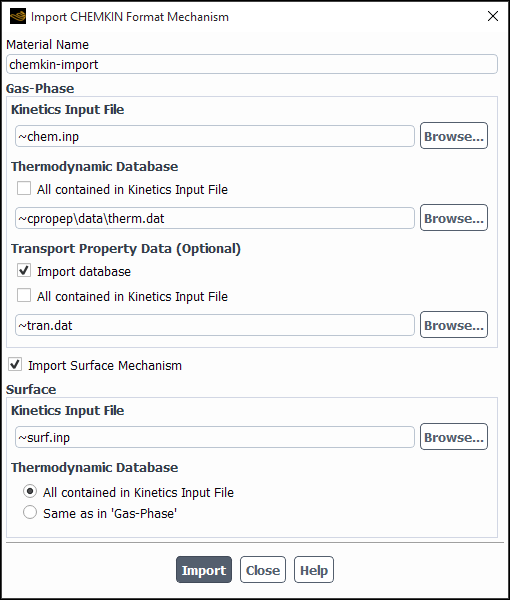
In the Import CHEMKIN Format Mechanism dialog box:
Enter a name for the chemical mechanism under Material Name.
Enable Import Surface Mechanism.
Enter the paths in the Kinetic Input File text fields in the Gas-Phase and Surface group boxes (for example,
path/chem.inp and path/path/surf.inp, respectively).Specify species thermodynamic property data. You can include the data in the kinetics input file and/or in a separate file as follows:
If you want to specify thermodynamic data for all species in the kinetics input file, enable All contained in Kinetics Input File to avoid the need to specify a separate file.
If you provide some or all species thermodynamic data in a separate file, disable All contained in Kinetics Input File and specify the thermodynamic data file location.
You can either use the default thermodynamic database file, thermo.db, provided in the cpropep\data directory in your Ansys Fluent installation area or specify the path of your thermodynamic database file if thermo.db does not contain all the gas-phase species in the CHEMKIN mechanism. The format for
thermo.dbis detailed in the CHEMKIN manual [79].To specify the surface species thermodynamic database, you can:
Select All contained in Kinetics Input File under the Thermodynamic Database and include the surface species thermodynamics data in the surface kinetics input file.
Select Same as 'Gas-Phase' and include the surface species thermodynamics data in the thermodynamics data file used in the gas-phase mechanism. Note that the default thermo.db file contains only gas-phase species. If you want to use this file, you will need to supply a thermodynamic database that includes surface species defined in your simulation.
Note: The surface species thermodynamic data must be included either in the surface kinetics input file or in the gas-phase thermodynamics data file. If you do not import thermodynamics data as a separate file in the gas-phase mechanism, then all surface thermodynamics data must be contained in the surface kinetics input file.
Click the button.
Ansys Fluent will create a material with the specified name, which will contain the CHEMKIN data for the species and reactions, and add it to the list of Fluent Mixture Materials. You can view all of the reactions by clicking the button to the right of Mechanism, under Properties in the Create/Edit Materials Dialog Box.
Ansys Fluent will also automatically save the imported data within the Fluent case file. Note that carrying the original input files along with the Fluent case file is not required. Ansys Fluent will automatically retrieve these files when needed (for example, when using the CHEMKIN-CFD solver).
For details on importing gas species transport properties, see Procedure for Importing Volumetric CHEMKIN Mechanisms.
Important: A surface reaction rate constant can be expressed in terms of a sticking coefficient in CHEMKIN mechanisms. When Stiff Chemistry Solver is selected from the Chemistry Solver drop-down list, Ansys Fluent will convert this sticking coefficient form to an equivalent Arrhenius rate expression [78]. For full compatibility with Ansys Chemkin, select CHEMKIN-CFD Solver instead.
Generally, Ansys Fluent handles all reaction types that are supported in Ansys Chemkin. However, some limitations still exist for the following models and features:
the None – Explicit Source chemistry solver (non-stiff chemistry)
the Finite-Rate/Eddy-Dissipation turbulence-chemistry interaction
In these cases, only the following volume reaction types can be used:
Arrhenius, including those reactions with arbitrary reaction order, third-body efficiencies and non-integer stoichiometric coefficients
Pressure-dependent reactions using the Lindemann, Troe and SRI forms
CHEMKIN mechanism files with CHEMKIN-default rate parameter units
Duplicate reactions (keyword DUP)
Arbitrary reverse reaction (keyword REV)
As with volume reactions, Ansys Fluent generally handles all reaction types that are supported in Ansys Chemkin. However, with the None – Explicit Source chemistry solver or Finite-Rate/Eddy-Dissipation turbulence-chemistry interaction, only the following surface reaction types can be used:
Arrhenius reactions, including those with arbitrary reaction order, third-body efficiencies and non-integer stoichiometric coefficients
Sticking coefficients (keyword STICK). Ansys Fluent converts these to an equivalent Arrhenius expression.
Arbitrary reaction units
Duplicate reactions (keyword DUP)
Surface coverage modification (keyword COV)
For a detailed description of the keywords, see Ansys Chemkin Input Manual.
The basic steps for setting up a problem involving wall surface reactions are the same as those presented in Overview of User Inputs for Modeling Species Transport and Reactions for setting up a problem with only fluid-phase reactions, with a few additions:
In the Species Model Dialog Box:
Setup → Models → Species Edit...
Enable Species Transport, select Volumetric and Wall Surface under Reactions, and specify the Mixture Material. See Enabling Species Transport and Reactions and Choosing the Mixture Material for details about this procedure, and Mixture Materials for an explanation of the mixture material concept.
(optional) If you want to model the heat release due to wall surface reactions, enable the Heat of Surface Reactions option.
(optional) If you want to include the effect of surface mass transfer in the continuity equation, enable the Mass Deposition Source option. When the density-based solver is used, this option is always enabled.
To control the robustness and the convergence speed, enter a value between 0 and 1 for the Aggressiveness Factor. A value of 0 is the most robust, but results in the slowest convergence. The default value for the Aggressiveness Factor is 0.5. This parameter appears only when the pressure-based solver is used.
(optional) If you are using the pressure-based solver and you want to include species diffusion effects in the energy equation, enable the Diffusion Energy Source option. See Wall Surface Mass Transfer Effects in the Energy Equation for details.
(optional, but recommended for CVD) If you want to model full multicomponent (Stefan-Maxwell) diffusion or thermal (Soret) diffusion, enable the Full Multicomponent Diffusion or Thermal Diffusion option. See Full Multicomponent Diffusion in the Fluent Theory Guide for details.
Check and/or define the properties of the mixture. See Defining Properties for the Mixture and Its Constituent Species.
Setup → Materials
Mixture properties include the following:
species in the mixture
reactions
other physical properties (for example, viscosity, specific heat)
Important:You will find all species (including the solid/bulk and site species) in the list of Fluent Fluid Materials. For a deposited species such as Si, you will need both Si(g) and Si(s) in the materials list for the fluid material type.
Note that the final gas-phase species named in the Selected Species list should be the carrier gas. This is because Ansys Fluent will not solve the transport equation for the final species. Note also that any reordering, adding or deleting of species should be handled with caution, as described in Assigning the Last Species.
Check and/or set the properties of the individual species in the mixture. (See Defining Properties for the Mixture and Its Constituent Species.) Note that if you are modeling the heat of surface reactions, you should be sure to check (or define) the formation enthalpy for each species.
Set species boundary conditions.
Setup → Boundary Conditions
In addition to the boundary conditions described in Defining Cell Zone and Boundary Conditions for Species, you will first need to indicate whether or not surface reactions are in effect on each wall. If so, you will then need to assign a reaction mechanism to the wall. To enable the effect of surface reaction on a wall, enable the Reaction option in the Species section of the Wall dialog box.
Important: If you have enabled the global Low-Pressure Boundary Slip option in the Viscous Model Dialog Box, the Shear Condition for each wall will be reset to No Slip even though the slip model will be in effect. Note that the Low-Pressure Boundary Slip option is available only when the Laminar model is selected in the Viscous Model dialog box.
See Inputs at Wall Boundaries for details about boundary condition inputs for walls. See User Inputs for Porous Media for details about boundary condition inputs for porous media.
In the surface reaction boundary condition described above, the effects of the wall normal velocity or bulk mass transfer to the wall are not included in the computation of species transport. The momentum of the net surface mass flux from the surface is also ignored because the momentum flux through the surface is usually small in comparison with the momentum of the flow in the cells adjacent to the surface. However, you can include the effect of surface mass transfer in the continuity equation by activating the Mass Deposition Source option in the Species Model Dialog Box. With the density-based solver, the effect of surface mass transfer in the continuity equation is always included.
Species diffusion effects in the energy equation due to wall surface reactions are included in the normal species diffusion term described in Treatment of Species Transport in the Energy Equation in the Theory Guide.
If you are using the pressure-based solver, you can neglect this term by disabling the Diffusion Energy Source option in the Species Model Dialog Box. For the density-based solvers, this term is always included; you cannot disable it. Neglecting the species diffusion term implies that errors may be introduced to the prediction of temperature in problems involving mixing of species with significantly different heat capacities, especially for components with a Lewis number far from unity. While the effect of species diffusion should go to zero at Le = 1, you may see subtle effects due to differences in the numerical integration in the species and energy equations.
The heat release due to a wall surface reaction is, by default, ignored by Ansys Fluent. You can, however, choose to include the heat of surface reaction by activating the Heat of Surface Reactions option in the Species Model Dialog Box and setting appropriate formation enthalpies in the Edit Material Dialog Box.
As in all CFD simulations, your surface reaction modeling effort may be more successful if you start with a simple problem description, adding complexity as the solution proceeds. For wall surface reactions, you can follow the same guidelines presented for fluid-phase reactions in Solution Procedures for Chemical Mixing and Finite-Rate Chemistry.
In addition, if you are modeling the heat release due to surface reactions and you are having convergence trouble, you should try temporarily turning off the Heat of Surface Reactions and Mass Deposition Source options in the Species Model Dialog Box.
If you are modeling surface site species, good estimates of the Initial Site Coverage will aid convergence.
In addition to the gas-phase variables listed in Postprocessing for Species Calculations, for surface reactions you can display/report the surface coverage as well as the deposition rate of the solid species deposited on a surface. Select Surface Coverage of species-n, Surface Deposition Rate of species-n, or Porous Deposition Rate of species-n in the Species... category of the variable selection drop-down list.
Important: For surface reactions involving porous media, you can display/report the surface reaction rates using the Kinetic Rate of Reaction-n(Porous) in the Reactions... category of the variable selection drop-down list.
Information about using particle reactions is divided into the following sections:
As described in The Multiple Surface Reactions Model in the Theory Guide, it is possible to define multiple particle surface reactions to model the surface combustion of a combusting discrete-phase particle. For more information about the theoretical background of particle surface reactions, see Combusting Particle Surface Reactions in the Theory Guide. Information about using particle surface reactions is provided in the following subsections:
Note the following limitations of the multiple surface reactions model:
The model is available only with the species transport model for volumetric reactions, and not with the nonpremixed, premixed, or partially premixed combustion models.
The multiple surface reactions model for combusting particles cannot be used with the breakup, collision and coalescence discrete phase models.
The setup procedure for particle surface reactions requires only a few inputs in addition to the procedure for volumetric reactions described in Overview of User Inputs for Modeling Species Transport and Reactions – Defining Other Sources of Chemical Species. These additional inputs are as follows:
In the Species Model dialog box, enable the Particle option under Reactions.
Setup → Models →
Species Edit...
When you specify the species involved in the particle surface reaction, be sure to identify the surface species, as described in Defining Properties for the Mixture and Its Constituent Species.
Important: You will find all species (including the surface species) in the list of Fluent Fluid Materials. If, for example, you are modeling coal gasification, you will find solid carbon, C(s), in the materials list for the fluid material type.
For each particle surface reaction, select Particle as the Reaction Type in the Reactions dialog box, and specify the following parameters (in addition to those described in Defining Reactions):
- Diffusion-Limited Species
When there is more than one gaseous reactant taking part in the particle surface reaction, the diffusion-limited species is the species for which the concentration gradient between the bulk and the particle surface is the largest. See Figure 7.1: A Reacting Particle in the Multiple Surface Reactions Model in the Theory Guide for an illustration of this concept. In most cases, there is a single gas-phase reactant and the diffusion-limited species does not need to be defined.
- Catalyst Species
This option is available only when there are no solid species defined in the stoichiometry of the particle surface reaction. In such a case, you will need to specify the solid species that acts as a catalyst for the reaction. The reaction will proceed only on the particles that contain this solid species. See Using the Multiple Surface Reactions Model for Discrete-Phase Particle Combustion for details on defining the particle surface species mass fractions.
- Diffusion Rate Constant
(
 in Equation 7–104 in the
Theory Guide)
in Equation 7–104 in the
Theory Guide)- Effectiveness Factor
(
 in Equation 7–102 in the
Theory Guide)
in Equation 7–102 in the
Theory Guide)
The catalytic particle surface reaction option is enabled in Ansys Fluent when Particle is selected as the Reaction Type in the Reactions Dialog Box and there are no solid species in the reaction stoichiometry. The solid species acting as a catalyst for the reaction is defined in the Reactions dialog box. The catalytic particle surface reaction will proceed only on those particles containing the catalyst species.
When you use the multiple surface reactions model, the procedure for setting up a problem involving a discrete phase is slightly different from that outlined in Steps for Using the Discrete Phase Models. The revised procedure is as follows:
Enable any of the discrete phase modeling options, if relevant, as described in Physical Models for the Discrete Phase Model.
Specify the initial conditions, as described in Setting Initial Conditions for the Discrete Phase.
Define the boundary conditions, as described in Setting Boundary Conditions for the Discrete Phase.
Define the material properties, as described in Setting Material Properties for the Discrete Phase.
Important: You must select multiple-surface-reactions in the Combustion Model drop-down list in the Create/Edit Materials dialog box before you can proceed to the next step.
If you have defined more than one particle surface species, for example, carbon (C<s>) and sulfur (S<s>), you will need to return to the Set Injection Properties dialog box (or Set Multiple Injection Properties dialog box) to specify the mass fraction of each particle surface species in the combusting particle. Click the Multiple Reactions tab, and enter the Species Mass Fractions. These mass fractions refer to the combustible fraction of the combusting particle, and should sum to 1. If there is only one surface species in the mixture material, the mass fraction of that species will be set to 1, and you will not specify anything under Multiple Surface Reactions.
Set the solution parameters and solve the problem, as described in Solution Strategies for the Discrete Phase.
Examine the results, as described in Postprocessing for the Discrete Phase.
Important: Solid deposition reactions on the particle are not allowed together with custom laws.
To model multicomponent particles with chemical reactions, you should follow the steps described in Steps for Using the Discrete Phase Models to setup multicomponent particle injections, with the modifications to the setup procedure outlined below. For more information about the theoretical background of the multicomponent particle reactions, see Multicomponent Particles with Chemical Reactions in the Fluent Theory Guide.
In the Species Model dialog box, enable both the Volumetric and Particle options (Reactions group box). This will enable multicomponent particle modeling.
In the Set Injection Properties dialog box, create an injection of the Multicomponent particle type.
In the Create/Edit Materials dialog box, define the following materials:
mixture
particle-mixture
Note:You can either compose your own mixture and particle-mixture materials or use one of the following predefined mixture and particle-mixture pairs from the Fluent database materials:
Calcium-carbonate-decomposition and calcium-carbonate-calcium-oxide
Urea-water-deposits-air-brack and urea-water-deposits
The multicomponent particle may contain reacting, volatile, or inert components that do not participate in any reactions.
For the particle-mixture material, select multicomponent-reactions from the Reaction Model drop-down list (Properties group box).
The Information dialog box will notify you that the multicomponent particle reactions must be specified in the Reactions dialog box for the mixture material.
Specify the components of the mixture and particle-mixture materials in the Species dialog box (accessed by clicking next to Mixture Species (Properties group box)).
When the multicomponent-reactions is used as the reaction model, then the Available Materials list is populated with both the fluid and droplet-particle materials for the mixture and the particle-mixture materials. In particular, for the particle-mixture material, the Available Materials list contains the fluid materials listed in the Selected Solid/Condensed Species list for the mixture material (see Figure 19.18: The Species Dialog Box for the Mixture Material and Figure 19.19: The Species Dialog Box for the Particle-Mixture Material with Reacting Components).
Reacting components must be included in the Selected Solid/Condensed Species list of the Species dialog box for the mixture material, and the particle species participating in reactions must be added to the Selected Species list for the particle-mixture material as shown below.
Note: The reacting components included in the Selected Solid/Condensed Species list of the Species dialog box for the mixture material are assumed to be in solid state, and consequently the viscosity and surface tension properties are not available in the Create/Edit Materials dialog box.
As an exception, generic values of viscosity and surface tension of the materials urea-liquid, biuret-liquid, and isocyanic-acid-liquid of the predefined urea-water-deposits and urea-water-deposits-air-brack mixture materials can be specified using the text command:
define/models/dpm/options/scr-urea-deposition/set-liquid-propertiesFor the mixture material, define particle reactions in the Reactions dialog box (accessed by clicking next to the Reaction drop-down list). See Inputs for Reaction Definition for more information.
In the Reaction Type group box, enable Particle.
Specify parameters for each reaction. Note that reactions can include particle species or gas phase species as either reactants or products.
In the Particle Reaction group box, select the particle reaction Model from one of the following options:
kinetics/diffusion
Calculates the reaction rate according to Ansys Fluent Model Formulation in the Fluent Theory Guide. This is the same model used for the combusting particle material when the multiple-surface-reactions option is selected as the Combustion Model in the Create/Edit Materials dialog box. For information about the kinetics/diffusion model parameters, see User Inputs for Particle Surface Reactions.
surface-kinetics
Calculates the reaction rate by Equation 7–112 in the Fluent Theory Guide.
volume-kinetics
Calculates the reaction rate according to Equation 7–114 in the Fluent Theory Guide
phase-change
Calculates the reaction rate according to Equation 7–115 in the Fluent Theory Guide
thermolysis
Calculates the thermolysis reaction rate according to Equation 7–116 in the Fluent Theory Guide. Note that the thermolysis reaction only occurs in freestream particles, and not in the Lagrangian wall-film particles.
user-defined
Allows you to specify a custom particle reaction using the
DEFINE_PR_RATEuser-defined function (UDF). SeeDEFINE_PR_RATEin the Fluent Customization Manual for details.
In the Species Model dialog box, make sure that the mixture material with the particle reactions is selected as the Mixture Material (Mixture Properties group box).
In the Set Injection Properties dialog box, configure the following settings:
Select the particle-mixture from the Material drop-down list.
In the Components tab, specify the multicomponent particle composition.
Note the following:
If a gas phase species is selected from the Evaporating Species dropdown list, this component is considered volatile and will evaporate according to Multicomponent Particle Definition (Law 7) in the Fluent Theory Guide.
If none is selected for the Evaporating Species, the component is available to participate in particle reactions or is inert/non-reacting.
The chemical reactions begin after all components with a corresponding gas phase species selected in the Evaporating Species drop-down list have evaporated.
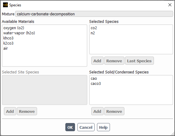
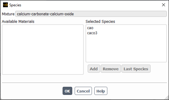
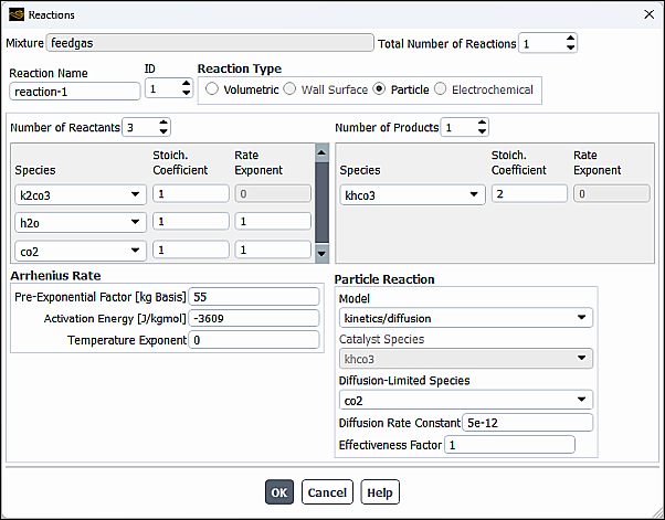
Note: It is recommended that for complex reaction mechanisms, you enable Multicomponent in the Coupled Heat-Mass Solution group box of the Discrete Phase Model dialog box (Numerics tab).
Once the solution is completed, the mass fractions of reacting and non-reacting components will be available for postprocessing similar to other particle variables.
Similar to wall surface reactions, electrochemical reactions generate sources (and sinks) in chemical species transport equations.
For more information about the theoretical background of electrochemical reactions, see Electrochemical Reactions in the Fluent Theory Guide. Information about using electrochemical reactions is presented in the following sections:
- 19.1.4.1. Overview and Limitation of Electrochemical Reactions
- 19.1.4.2. User Inputs for Electrochemical Reactions
- 19.1.4.3. Electrochemical Reaction Effects in the Energy Equation
- 19.1.4.4. Electrochemical Reaction Effects in the Species Transport Equation
- 19.1.4.5. Including Mass Transfer in Continuity
- 19.1.4.6. Solution Procedures for Electrochemical Reactions
- 19.1.4.7. Modeling Corrosion with the Water Corrosion Pre Tool
An electrochemical reaction occurs only on wall surfaces where the electrolyte and the electrode meet. Both aqueous and solid species can participate in electrochemical reactions. Solid species that can be involved in electrochemical reactions are corroded or deposited species.
Electrochemical reactions can be limited, so that they can only occur on some of the wall boundaries (while the other wall boundaries remain free of reaction). The reaction rate is defined and computed per unit surface area, in contrast to the fluid-phase reactions, which are based on unit volume.
You can specify different reaction mechanisms for different walls. Each reaction mechanism can have multiple electrochemical reactions.
Electrochemical reactions are not available with the density-based solver.
The steps needed to incorporate electrochemical reactions in your problem are as follows:
For unsteady simulations, select Transient from the General task page (Solver group).
Enable chemical species transport model.
Setup → Models → Species Edit...
In the Species Model dialog box, under Model, enable Species Transport.
Under Reactions, select Volumetric and Electrochemical.
Note: Once you enable the Electrochemical reactions, the electric potential solver will be automatically enabled (under the Models tree branch).
In the Create/Edit Materials dialog box, define all the species materials that are present in the electrolyte and electrodes.
Setup → Materials
Copy the new species from the Fluent database to your case as described in Copying Materials from the Ansys Fluent Database. If your species material is not present in the database, copy a similar species material and edit its properties, including Name and Chemical Formula.
Note:When copying species (including corroded and deposited solid species), make sure that fluid is selected as Material Type in the Fluent Database Materials dialog box.
It is not necessary to represent the electron in the reaction, and
e-can be safely ignored.
Under the Properties group box, set Charge Number for the new species.
Important: By default, Charge Number is set to 0, which means that the species is neutral. Make sure to specify the Charge Number for all relevant species.
Note: Do not specify Electrical Conductivity for individual species. You will specify Electrical Conductivity for the mixture.
Edit the mixture composition using the Species dialog box (opened by clicking Edit next to Mixture Species under Properties of the Create/Edit Materials dialog box).
Remove unused species and add the electrochemical species to the Selected Species list as described in Adding Species to the Mixture.
If solid species are involved in the electrochemical reactions (for example, in corrosion or electroplating simulations), add them to the Selected Solid Species list.
Note: Make sure that the bulk species is the last species in the Selected Species list. Ansys Fluent solves transport equations for all but the last species in the Selected Species list. The order of the solution is the same as the order of the species in Selected Species.
Specify the reactions in the Reactions dialog box (opened by clicking Edit next to Reactions under Properties of the Create/Edit Materials dialog box).
For each reaction, configure the following settings:
Select Electrochemical as the reaction type.
If you want the Tafel Equation 7–119 in the Fluent Theory Guide, rather than the Bulter-Volmer Equation 7–118, to be used in the kinetics calculation, select Tafel Parameters.
Specify the following Butler-Volmer/Tafel Parameters:
Butler-Volmer parameters (the Tafel Parameters check box is cleared):
Anodic Transfer Coefficient (
 in Equation 7–118 in the Fluent Theory Guide)
Cathodic Transfer Coefficient (
 in Equation 7–118 in the Fluent Theory Guide)
Tafel parameters (the Tafel Parameters check box is selected):
Anodic Tafel Slope (
 in Equation 7–119 in the Fluent Theory Guide)
Cathodic Tafel Slope (
 in Equation 7–119 in the Fluent Theory Guide)
Exchange Current Density (
 in Equation 7–118 and Equation 7–119 in the Fluent Theory Guide)
Reference Temperature (
 in Equation 7–118 and Equation 7–119 in the Fluent Theory Guide)
Activation Energy (
 in Equation 7–118 and Equation 7–119 in the Fluent Theory Guide)
Equilibrium Potential (
 in Equation 7–120 in the Fluent Theory Guide)
You can define a constant, polynomial, piecewise-linear, or user-defined function for any of the aforementioned Butler-Volmer/Tafel parameters.
Enter the
 th species dimensionless
power (
th species dimensionless
power ( in Equation 7–118 in the Fluent Theory Guide) as Rate Exponent.
Under the Butler-Volmer/Tafel Parameters group box, click the button and in the Reference Molar Concentrations dialog box that opens (see Reference Molar Concentrations Dialog Box), enter the reference species molar concentrations (
 in Equation 7–118 in the Fluent Theory Guide).
The reference molar concentrations essentially act as scaling factors in the Butler-Volmer equation. In the literature, when a reaction mechanism is discussed, the authors usually provide values for the reference molar concentration as well as the current density and other kinetics parameters. In Ansys Fluent, the default value is 1 kmol/m3 for all the reference molar concentrations.
Note: You can customize the electrochemical reaction rate by using the following UDFs:
DEFINE_EC_KINETICS_PARAMETER: to customize an individual kinetics parameter in the Butler-Volmer reaction rateDEFINE_EC_RATE: to define a totally different function form for the reaction rate.
Refer to
DEFINE_EC_KINETICS_PARAMETERandDEFINE_EC_RATEin the Fluent Customization Manual for details about those functions.
Define reaction mechanisms using the Reaction Mechanisms dialog box (opened by clicking Edit next to Mechanism under Properties of the Create/Edit Materials dialog box).
Specify Number of Mechanisms. If you type in the value, be sure to press .
For each electrochemical reaction mechanism, configure the following settings:
Set the Mechanism ID of the mechanism you want to define. Again, if you type in the value, be sure to press .
Select Electrochemical as a reaction type.
Under Reactions, select the reaction and in the Name text entry field, specify a meaningful name for the mechanism (for example,
mechanism-anodeormechanism-cathode).
In the Create/Edit Materials dialog box, set the remaining mixture properties, such as Density (typically volume-weighted-mixing-law), Mass Diffusivity, and Electrical Conductivity.
Note that if the anode, cathode, and electrolyte have different material properties, such as species mass diffusivities, it is best to use a UDF. Alternatively, you can create new materials for the anode and cathode by copying existing materials from the Fluent database, renaming them, and then assigning these materials to the anode and cathode fluid zones in the Cell Zone Conditions dialog box.
For electrolyte and electrode zones, set cell zone conditions using Cell Zone Conditions Task Page.
Setup → Cell Zone Conditions In the Fluid dialog box, specify whether or not the selected zone is an electrolyte zone by selecting or clearing the Electrolyte check box. By default, all fluid zones are electrolyte zones.
If there is no volumetric reactions, clear the Reaction check box.
Set the electrochemical boundary conditions for all relevant walls using Boundary Conditions Task Page.
Setup → Boundary Conditions
Electrochemical reaction can be defined at either exterior (1-sided) walls or interior (2-sided) walls with only one side exposed to electrolyte.
In the Wall dialog box, configure the following settings:
For exterior (1-sided) walls, set the potential boundary conditions as described in Setting Up the Electric Potential Model.
Specify whether or not the wall is Faradaic by selecting or clearing the Electrochemical Reaction check box.
For Faradaic walls, from the Reaction Mechanism drop-down list, select the reaction mechanism that you have previously defined.
If the electrochemical reaction is defined on the wall (Electrochemical Reaction is selected), you can include the reaction heat in the energy equation by selecting the Faradaic Heat check box.
Note: For the 2-sided wall, you need to specify the potential boundary conditions only on one side of the wall. The settings you have specified will be automatically copied to the other side of the wall.
(optional) You can include additional sources in the energy, continuity, and species transport equations as described in the following sections:
Set the solution parameters in the Solution Methods Task Page and Solution Controls Task Page.
In many electrochemical applications, fluid convection can be neglected, in which case the Flow equation should be disabled in the Equations control box (accessible from the Solution Controls Task Page).
Similarly, for isothermal simulations, the Energy equation should be disabled.
Important: If the potential equation has difficulty converging, you can lower the Faradaic Interface Current under-relaxation factor in the Solution Controls task page to improve stability.
Once the solution is converged, you can display or report the following variables that are available under the Potential category:
Electric Potential
Electric Conductivity
Faradaic Current Density
Total Surface Corrosion Rate
Electrode Surface Potential
Current Density
Joule Heat Source
Faradaic Heat Source
Total Echem Heat Source
In addition, you can display
Echem Reaction Rate of each reactions (under the Reactions category)
Surface Corrosion Rate of each solid species on a wall (under Species category)
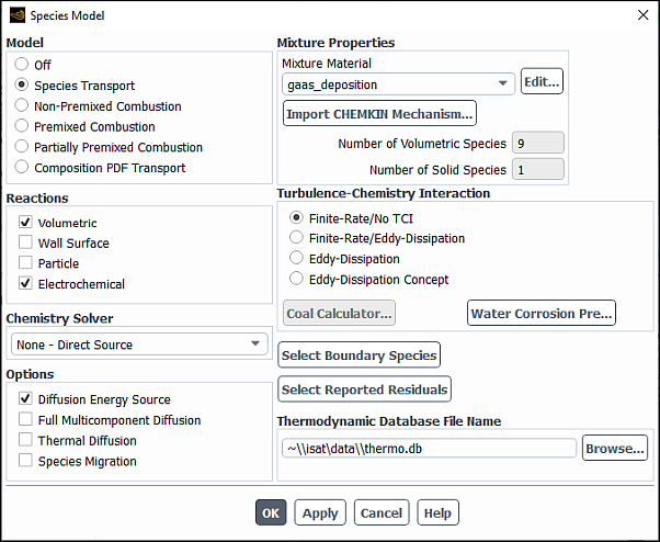
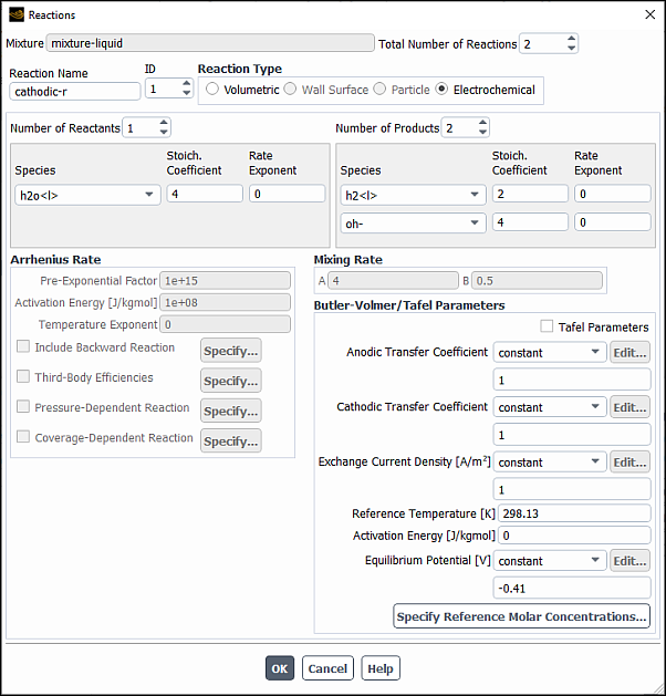
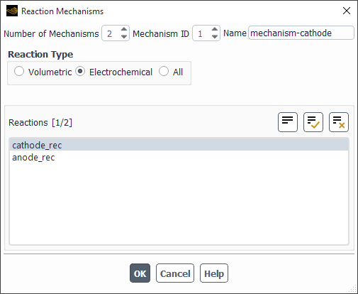
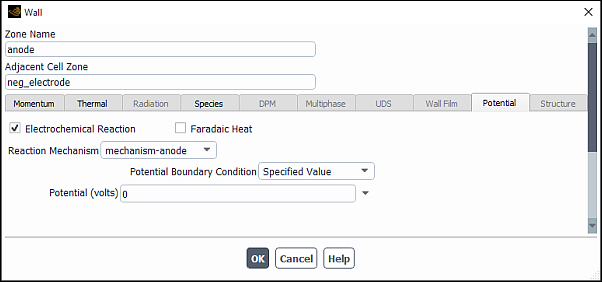
When the electrochemical reaction model is enabled, you can specify two extra sources in the energy equation:
Joule heating in the fluid and solid zones
You can include the Joule heating in the energy equation calculation by selecting the Include Joule Heating in Energy Equation option in the Electric Potential dialog box (Setting Up the Electric Potential Model).
Electrochemical reaction heat at Faradaic interfaces
You can include the electrochemical reaction heat by selecting the Faradaic Heat option in the boundary condition dialog boxes for each reacting wall.
When the electrochemical reaction model is enabled, you can specify an extra source in the species transport equation for the ion-species:
Species migration in the electric field
You can include this effect by selecting the Species Migration option in the Species Model Dialog Box.
When a solid species (corroded or deposited) is involved in an electrochemical reaction, the solid material can enter or leave the flow domain. Usually the mass transfer of the solid species is small and can be ignored in the continuity equation. However, if you want, you can include the mass source in the continuity equation by using the following Scheme command:
(rpsetvar ‘potential/corrosion-source-in-continuity?
#t)
The strongly nonlinear coupling between species and electric field can cause convergence problems. To improve the stability of the solution, you can lower the Faradaic Interface Current under-relaxation factor in the Solution Controls Task Page.
In addition, you can try temporarily disabling the Include Joule Heating in Energy Equation and Faradaic Heat options (see Electrochemical Reaction Effects in the Energy Equation).
You can enable these options once the solution becomes more stable.
One important electrochemical reaction application is corrosion. In the oil and gas industry, pipelines and processing equipment, which are made of mild steel, may be subject to the CO2 aqueous environment. As a result, the so called “sweet” CO2 corrosion may occur in such systems. Depending on the aqueous environment (strong acid or CO2), different homogenous volumetric reactions and heterogeneous electrochemical reactions can be present in the system.
The heterogeneous electrochemical reactions are the same for all the environments. The anodic reaction is the dissolution of iron in a water solution:
 | (19–9) |
The reaction rate is computed from the following Tafel equation:
 | (19–10) |
with the following parameter values taken from [106]:
 = 1 A/m2 = 1 A/m2 |
 = -0.488 V = -0.488 V |
 = 0.04 V = 0.04 V |
 = 37.5 kJ/mol = 37.5 kJ/mol |
 = 298.15 K = 298.15 K |
Refer to Equation 7–119 in the Fluent Theory Guide for the notation used in Equation 19–10.
The cathodic reaction is a hydrogen evolution reaction via the reduction of H+ ions:
 | (19–11) |
The charge transfer current density can be calculated using the Tafel equation as:
 | (19–12) |
with the following parameter values taken from [106]:
 = 0.03 A/m2 = 0.03 A/m2 |
 = -0.24 V = -0.24 V |
 = 0.12 V = 0.12 V |
 = 30 kJ/mol = 30 kJ/mol |
 = 298.15 K = 298.15 K |
 = 1.0e-4 M = 1.0e-4 M |
The homogeneous reactions are different depending on the environment:
Strong acid environment
In such environments, the acid is practically fully dissociated in water, and there is no need to solve any homogeneous reactions. The species involved in such systems include H+<l>, OH-<l>, Fe2+<l>, H2<l>, H2O<l>, and Fe<b>.
CO2 environment
When CO2 gas is dissolved in water, a series of chemical reactions occurs, and that may make the resultant solution corrosive to mild steel. The reactions in this environment are:
Each reaction is reversible. The reaction kinetics parameters for the forward and backward reactions are taken from [106]
The species involved in such systems include H+<l>, OH-<l>, CO2<l>, H2CO3<l>, HCO3-<l>, CO32-<l>, Fe2+<l>, H2<l>, H2O<l>, and Fe<b>.


The Water Corrosion Pre tool is designed to assist you in setting a corrosion case quickly in Ansys Fluent. Using this tool, you can conduct water chemistry calculation and create corresponding material and reactions for the environment.
The following procedure provides an overview of the steps required for setting up a corrosion case. Only the steps that are pertinent to corrosion simulations are shown here. For information about inputs related to other models that you want to use in your case, see the appropriate sections for those models in the Ansys Fluent User's Guide
In the Species Model dialog box, enable the Species Transport model, and in the Reactions group box, enable the following reactions:
Volumetric
Wall Surface
Electrochemical
Click the button.
In the dialog box that opens (see Figure 19.25: The Water Chemistry and Corrosion Mechanism Dialog Box), select the Reaction Type from the following options:
Strong Acid Environment
CO2 Environment
The species and reactions involved in the water chemistry for the selected reaction type are shown in the Species/Reactions group box. For additional information, see Background.
Specify Inputs for the selected reaction type.
For the CO2 Environment reaction type, you need to specify the following parameters:
- Density of Liquid
is the water solution density.
- Temperature
is the solution temperature at which the equilibrium calculation is carried out.
- Total Pressure
is the pressure used to calculate some of the water equilibrium constants.
- CO2 Partial Pressure
is the partial pressure of CO2 in the gas phase, which is used to calculate the aqueous phase (CO2) concentration in the CO2 dissolution reaction (CO2<g> <=> CO2<l>).
- Fixed pH Value?
when enabled, allows you to specify the pH Value of the solution.
- pH Value
is the pH value of the solution. This item is available only when Fixed pH Value? is enabled.
For the Strong Acid Environment reaction type, you need to specify only the following parameters:
Density of Liquid
pH Value.
Click the Compute Equilibrium button to initiate the water chemistry calculation.
The species concentration from the equilibrium calculation are printed to the Ansys Fluent console. They are also displayed in the Equilibrium Calculation Results group box of the dialog box. You can select to display the results in the following units:
Molar Concentration
Mass Fraction
Mole Fraction
The equilibrium calculation results are automatically passed to the corresponding boundary condition dialog boxes and Solution Initialization task page where the relevant fields are updated.
Click the Create Mixture Material and Reactions button to create a mixture material, reactions, and chemistry mechanisms for the selected reaction type.
Depending on the environment, one of the following materials is created:
mixture-strong-acid for Strong Acid Environment
mixture-co2-corrosion for CO2 Environment
For each mixture, all the species involved, reactions, and mechanisms are pre-defined. For the both environments, the following three electrochemical reaction mechanisms are created:
mechanism-anodic: Includes only the anodic reaction
mechanism-cathodic: Includes nly the cathodic reaction
mechanism-combined-echem: Includes both the anodic and cathodic reactions
For the CO2 environment, where some homogeneous reactions are present, a volumetric reaction mechanism, mechanism-volumetric, is also created. This mechanism can be assigned to a fluid zone.
In a galvanic corrosion, where anodic and cathodic reactions occur at different surfaces, the mechanism-anodic and mechanism-cathodic mechanisms can be assigned to the corresponding surfaces. In a uniform corrosion case, where the anodic and cathodic reactions occur at the same surface, the mechanism-combined-echem mechanism can be used.
In addition, Ansys Fluent automatically applies the following changes:
Sets the newly created material as the mixture material in the Species Model dialog box.
Assigns the newly created material to the fluid zone(s).
Updates the species mass fractions in the Species tab of the relevant boundary conditions dialog boxes.
Specify boundary conditions using the equilibrium calculation results.
Set boundary conditions for all species at all inlets
Hook the electrochemical reaction mechanism to all walls where corrosion occurs.
In the Fluid dialog box, specify cell zone conditions for the fluid zones. For the CO2 Environment reaction type, hook the mechanism-volumetric mechanism to all fluid zones where CO2 environment corrosion occurs.
Initialize the species field.
Run the simulation.
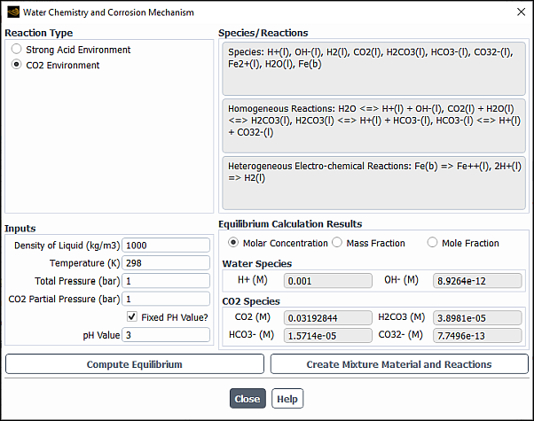
In addition to the volumetric and surface reactions described in the previous sections, you can also use Ansys Fluent to solve a species mixing problem without reactions. The species transport equations that Ansys Fluent will solve are described in Volumetric Reactions in the Theory Guide, and the procedure you will follow to set up the non-reacting species transport problem is the same as that described in Overview of User Inputs for Modeling Species Transport and Reactions – Defining Other Sources of Chemical Species, with some simplifications.
The basic steps are listed below:
Enable Species Transport in the Species Model dialog box and select the appropriate Mixture Material.
Setup → Models → Species Edit...
See Overview of User Inputs for Modeling Species Transport and Reactions for information about the mixture material concept, and Enabling Species Transport and Reactions and Choosing the Mixture Material for more details about using the Species Model dialog box.
(optional) If you want to model full multicomponent (Stefan-Maxwell) diffusion or thermal (Soret) diffusion, enable the Full Multicomponent Diffusion or Thermal Diffusion option.
Check and/or define the properties of the mixture and its constituent species.
Setup → Materials
Mixture properties include the following:
species in the mixture
other physical properties (for example, viscosity, specific heat)
See Defining Properties for the Mixture and Its Constituent Species for details.
Set species boundary conditions, as described in Defining Cell Zone and Boundary Conditions for Species.
No special solution procedures are usually required for a non-reacting species transport calculation. Upon completion of the calculation, you can display or report the following quantities:
Mass fraction of species-n
Mole fraction of species-n
Concentration of species-n
Lam Diff Coef of species-n
Eff Diff Coef of species-n
Enthalpy of species-n (pressure-based solver calculations only)
Relative Humidity (when the water vapors (H2O) is present in the species mixture material)
Mean Molecular Weight
Liquid species mass fraction of species-n (solidification and melting model only)
These variables are contained in the Species... and Properties... categories of the variable selection drop-down list that appears in postprocessing dialog boxes. See Field Function Definitions for a complete list of flow variables, field functions, and their definitions. Displaying Graphics and Reporting Alphanumeric Data explain how to generate graphics displays and reports of data.
Information about using the reacting channel model is presented in the following subsections. For more information about the theoretical background, see Reacting Channel Model in the Theory Guide.
The reacting channel model in Ansys Fluent offers an efficient solution methodology for solving reacting flow in shell and tube heat exchangers with long and thin channels. The volume inside the reacting channels is not meshed and solved with the outer flow. Instead, a plug flow approximation is used for the reacting channels, which is coupled to the outer flow through heat transfer across the channel walls.
The reacting channel model has the following limitations:
The reacting channel model is available only for steady-state 3D problems.
Shell conduction cannot be used on reacting channel walls.
The reacting channel model solves the one-dimensional species equations at the centerline of the reacting channel. The accuracy of the model depends on how well Ansys Fluent computes the channel centerline from the channel wall surface mesh. It is highly recommended to use a swept structured surface mesh on the channel wall (see Figure 19.26: Optimal Surface Mesh on the Reacting Channel Wall). Unstructured channel wall surface meshes may result in loss of accuracy due to inconsistent channel centerlines.
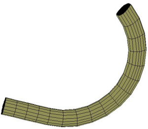
The steps and procedure to set up a reacting channel model are outlined below. In this section, the steps pertinent to the reacting channel model only are explained. The setting up of other models used in conjunction with reacting channel models are explained in other sections of the User's Guide.
Enable the reacting channel model.
Setup → Models →
Species → Reacting Channel Model
Edit...
When you enable the Enable Reacting Channel Model option, the dialog box will expand to show the relevant inputs (see Figure 19.27: The Reacting Channel Model Dialog Box).
Specify the Number of Boundary Groups. If you have multiple channels, you can group together channels with common flow direction, mixture materials, inlet compositions, temperature, pressure, and mass flow rate. You will be required to provide the inputs for each boundary group.
Note: If you have multiple tubes, you will need to define each tube as a different wall and set up the model by grouping the walls together if they have the same boundary conditions.
Enter the number of Flow Iterations Per Coupling Iteration. This is the number of outer flow iterations for each channel flow iteration.
Optionally change an Under-Relaxation Factor. The value of the under-relaxation factor is used to update the heat flux from the reacting channel. See Equation 7–145 in the Theory Guide.
Set the Group Index. Note that the Group Index for the first boundary group is set to
0.The inputs for each boundary group are entered in the Group Settings and Group Inlet Conditions tabs as further described.
Under the Group Settings tab, specify the model settings and options. (see Figure 19.28: The Reacting Channel Model Dialog Box (Group Inlet Conditions Tab)).
In the Channel Walls in Group selection list, select the wall boundary zones that correspond to the reacting channels.
Select the group material from the Material drop-down list. You can choose any mixture material available in the case as a group material.
Optionally, import a CHEMKIN mechanism using button. For details see Importing a Volumetric Kinetic Mechanism in CHEMKIN Format.
To model surface reactions within the channel, enable Surface Reactions under Model Options group box. The dialog box will expand to show the related inputs as shown in Figure 19.27: The Reacting Channel Model Dialog Box. These inputs include:
Surface to Volume Ratio of the channel group
Surface reaction mechanism of the group (selected from the Reaction Mechanism drop-down list)
To model porous medium, enable Porous Medium under Model Options group box. The dialog box will expand to show porous medium inputs as shown in Figure 19.27: The Reacting Channel Model Dialog Box. These inputs include:
Porosity of the channel
Viscous Resistance in axial direction of the channel
Inertial Resistance in axial direction of the channel
Solid material of the porous medium inside the channel (selected from the Solid Material drop-down list)
Under the Group Inlet Conditions tab, specify the inlet conditions for the boundary group (see Figure 19.28: The Reacting Channel Model Dialog Box (Group Inlet Conditions Tab)). You can specify the inlet condition parameters as constant values. Ansys Fluent provides you also with the option of redefining any or all of the inlet condition parameters using user-defined functions (UDFs).
Specify the X-, Y-, and Z-component of the flow at the inlets of the channels in the current group in the Flow Direction group box.
Note: Since there is no surface or zone to identify the channel inlet or outlet, the inlet flow direction of the group is used to determine the channel inlet. Therefore, It is very important to specify the flow direction correctly.
Enter the inlet channel Temperature, Flow Rate and Pressure in the group.
Specify the inlet mass fractions for each species in the group in the Species Composition group box.
To specify an inlet condition using a user-defined function (UDF), select the User Defined Inlet Conditions check box and then select the appropriate user-defined function from the drop-down list. For information about specifying and hooking DEFINE_REACTING_CHANNEL_BC UDFs, see
DEFINE_REACTING_CHANNEL_BCin the Fluent Customization Manual.
Click the button to save the settings.
If you specified more than one boundary group in step 1, change the group ID value in Group Index integer number entry box and repeat steps 5–7 for each remaining boundary group.
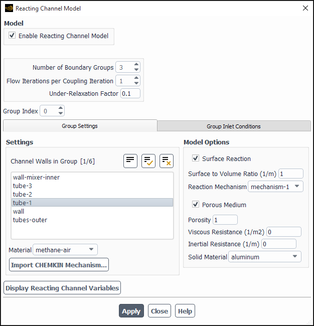
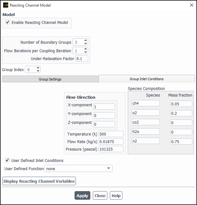
Once the reacting channel model is defined, you can generate reports or plots of reacting channel variables using the Reacting channel 2D Curves dialog box (Figure 19.30: Reacting Channel 2D Curves Dialog Box (Plot)). You can open the Reacting channel 2D Curves dialog box by clicking the button in the Reacting Channel Model dialog box. For information about the plotting of reacting channel model variables, see Postprocessing for Reacting Channel Model Calculations.
Modeling Curvilinear Reacting Channels
In the reacting channel model, the two ends of a channel are identified as the inlet and the outlet based on the inputs provided for the inlet flow direction of the group. However, for some special channel configurations, such as U-tubes, it is not possible to identify the inlet/outlet of the channel based on the information of the inlet flow direction. For such cases, an additional input is required to differentiate between the end points of the channel as inlet or outlet. The additional input is to provide the centroid coordinates of the inlet of the U shaped channel. Therefore, for U-tube configurations, after setting up the reacting channel model following the earlier steps in this section, it is required to use the following text user interface commands to set the inlet and outlets correctly:
/define/models/species> reacting-channel-model-options
Are any of the channels a U-tube configuration? [no] yes
Is wall tube1 a U-tube configuration? [no] yes
Enter the coordinates of the center of the inlet for wall tube1
X coordinate [0] 0.01
Y coordinate [0] 0
Z coordinate [0] 0
Where tube1 is
a reacting channel wall having a U shape. You will be asked the same
questions for each of the existing reacting channel walls.
In the Ansys Fluent wall boundary conditions dialog box, the wall surfaces that you selected as channel walls in the Reacting Channel Model dialog box will have zero heat flux boundary conditions, which are disabled as shown in Wall Surface Reactions and Chemical Vapor Deposition).
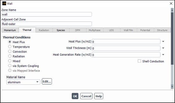
The heat flux at the channel walls is calculated internally through the coupling of the reacting channel model with the outer flow as described in Reacting Channel Model in the Theory Guide. For all other wall surfaces, which are not channel walls, all boundary conditions as described in Wall Boundary Conditions are applicable.
Ansys Fluent provides postprocessing options for plotting and reporting channel variables using the Reacting Channel 2D Curves dialog box that opens by clicking the button in the Reacting Channel Model dialog box. You can generate X-Y plots or reports of the following reacting channel variables:
Bulk mean temperature of the channel
Wall temperature of the channel
Nusselt Number (for the channel wall on the channel side)
Wall heat flux through the channel walls
Velocity inside the channel
Density of the channel
Mass fraction of the species inside the channel
The surface coverage and the deposition rate of the surface species.
The steps for generating the plots/reports are as follows:
Select either Plot Reacting Channel Variables or Report Reacting Channel Outlet Average.
The Reacting Channel 2D Curves dialog box displays either the Variable Name drop-down list for selecting a single species for X-Y plot generation, or the Variable Names selection list for selecting multiple species for report generation as shown in Figure 19.30: Reacting Channel 2D Curves Dialog Box (Plot) and Figure 19.31: Reacting Channel 2D Curves Dialog Box (Report).
Specify whether you want to write the plot data to a file by using the Write To File check box.
If more than one boundary group is defined for reacting channel model, specify the group ID in the Group Index integer number entry box.
The Variable Name drop-down/Variable Names selection list contains reacting channel variables of the specified boundary group. Select the reacting channel variable(s) from the list.
Select the wall surface(s) from the Wall Surfaces selection list on which the plot/report will be generated (at least one wall surface must be selected).
Click one of the following as applicable:
Plot to view X-Y plot in the graphics window
Print to view report in the console window
Write... to save to file
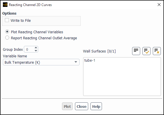
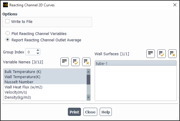
Information about using the Reactor Network model is presented in the following subsections.
For more information about the theoretical background, see Reactor Network Model in the Fluent Theory Guide.
The Reactor Network model allows rapid solution of combustors using detailed chemical kinetic mechanisms. This speed is achieved by first performing a Fluent CFD simulation with a fast chemistry model, such as a Non-Premixed, Partially-Premixed, or Eddy-Dissipation model, and then using the Reactor Network model to solve with a detailed kinetic mechanism. The Reactor Network model agglomerates cells from the CFD solution into a user-specified small number of reactors and computes detailed chemistry on this reactor network.
Since the chemical kinetics is decoupled from the flow, reactor network simulations are applicable to steady simulations where the chemical kinetics does not affect the flow significantly, such as pollutant formation. Inherently unsteady simulations, such as ignition and global extinction, cannot be modeled with reactor networks. Note that the Reactor Network model can be used for unsteady simulations of statistically steady flows, such as LES, where the time-averaged flow and species fields are used to construct the reactor network.
The steps and procedure for setting up and solving a Reactor Network model are outlined below.
Enable the Reactor Network model.
Setup → Models → Species → Reactor Network Edit...
Important: Note that this model is only available when one of the reacting species models is enabled.
When you select the Reactor Network Model option, the dialog box expands to show the relevant modeling controls (see Figure 19.32: Reactor Network Dialog Box (Steady-State Flow)).
If a detailed chemical mechanism has already been imported, select the mixture material from the Detailed Mechanism Material Name drop-down list. Otherwise import a mechanism in CHEMKIN format by clicking Import CHEMKIN Mechanism.... The mechanism files are imported into your case using the Import CHEMKIN Format Mechanism dialog box as described in Specifying a Chemical Mechanism File for Flamelet Generation.
Set the Number of Reactors in the reactor network. The default value of 50 is a good starting value, but it can be increased for greater accuracy.
Specify whether or not the temperature is calculated from the equation of state by selecting or clearing the Solve Temperature check box. By default, this option is selected, and Ansys Fluent will determine the temperatures in the reactor network.
Once cells are agglomerated and a reactor-network solution is calculated, you can select the Use Current Reactor Network option to perform further reactor network simulations with the existing network of connected reactors. This option can be used to continue iterations from the previous reactor- network solution if additional convergence is desired. The option also allows you to change the chemical mechanism or species boundary conditions to generate a new solution on the current reactor network.
(for transient analysis with the Data Sampling For Time Statistics option selected in the Run Calculation task page only) Specify whether or not you want to use the time-averaged composition fields to agglomerate the reactors and time-averaged velocity fields to calculate the reactor mass flux matrix (instead of the instantaneous fields) by selecting or clearing the Use Time Averaged Fields option.
Note: The Use Time Averaged Fields option should be used for unsteady simulations (for example, LES) of statistically stationary combustors.
If necessary, specify custom-field functions and adjust the default solver settings using the Expert Options control. When Expert Options is selected, the Reactor Network dialog box expands to reveal the following advanced options:
- ODE Relative Error Tolerance, ODE Absolute Error Tolerance
The default values for the ODE relative and absolute error tolerances are 1e-05 and 1e-12, respectively. If the ODE solver fails to converge, it is often helpful to lower the ODE Relative Error Tolerance and the ODE Absolute Error Tolerance.
- Reactor Network Convergence Tolerance
The default value for the reactor network convergence tolerance is 1e-08. Residuals should be well converged at the default tolerance. Higher tolerances may be acceptable for engineering accuracy.
- Solver
The default segregated solver typically converges faster than the coupled solver. However, when using the segregated solver, residuals may stall above an acceptable tolerance. In this case, the coupled solver should be used.
- Maximum Number of Iterations (segregated solver)
If residuals are still decreasing and better convergence is desired, increase the maximum number of iterations. If residuals are stalled and a quicker exit from the solver is desired, decrease the maximum number of iterations.
- Maximum Integration Time (coupled solver)
The ODE solver terminates the calculation at this time if residuals fail to converge.
- Use Custom Field Functions to Define Reactor Zones
When selected, this option allows you to use custom field functions (Custom Field Functions) as composition variables to create the reactor volumes. Ansys Fluent clusters CFD cells that have similar compositions using the following default composition variables:
temperature and mixture fraction for Non-Premixed and Partially-Premixed cases
temperature and mass fractions of N2 and H2O for Species Transport cases
You can override these default composition variables by selecting Use Custom Field Functions to Define Reactor Zones and then selecting up to four custom field functions from the Custom Field Functions selection list. Ansys Fluent will group CFD cells that are close in these custom field function composition variables. In the example shown in Figure 19.33: Reactor Network Dialog Box - Expert Options, cells with similar turbulent kinetic energy, x coordinate, and y coordinate will be agglomerated to form the reactor network.
Click Calculate Reactor Network to obtain a flow solution.
As the calculation is progressing, Ansys Fluent prints the reactor network residuals for each iteration in the console.
Note: The reactor network solution should converge with the default settings. However, if the model fails to converge with sufficient accuracy, you can adjust the default reactor network solver settings by using the Expert Options control.
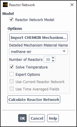
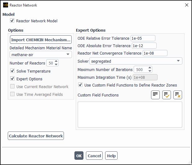
Ansys Fluent provides additional postprocessing options for reactor network calculations. The following reactor network variables are available for generating graphical plots:
Reactor Net Zone ID
Reactor Net Temperature
Reactor Net Mass fraction of species-n
These variables will appear under the Reactor Network… postprocessing category of the variable selection drop-down lists.