


The procedure for setting up and solving a general multiphase problem is outlined below, and described in detail in the subsections that follow. Remember that only the steps that are pertinent to general multiphase calculations are shown here. For information about inputs related to other models that you are using in conjunction with the multiphase model, see the appropriate sections for those models.
See also Additional Guidelines for Eulerian Multiphase Simulations for guidelines on simplifying Eulerian multiphase simulations.
Important: Double Precision is recommended for all multiphase cases.
Enable the multiphase model you want to use (VOF, mixture, or Eulerian) and specify the number of phases. For the VOF and Eulerian models, specify the volume fraction scheme as well.
 Setup → Models →
Multiphase
Setup → Models →
Multiphase  Edit...
See Enabling the Multiphase Model and Choosing Volume Fraction Formulation for details.
Copy the material representing each phase from the materials database.
Setup →  Materials
If the material you want to use is not in the database, create a new material. See Using the Create/Edit Materials Dialog Box for details about copying from the database and creating new materials. See Modeling Compressible Flows for additional information about specifying material properties for a compressible phase. It is possible to turn off reactions in some materials by selecting none in the Reactions drop-down list under Properties in the Create/Edit Materials dialog box.
Important: If your model includes a particulate (granular) phase, you will need to create a new material for it in the fluid materials category (not the solid materials category).
Define the phases, and specify any interaction between them (for example, surface tension if you are using the VOF model, slip velocity functions if you are using the mixture model, or drag functions if you are using the Eulerian model).
Setup → Models
→ Multiphase Edit...
See Defining the Phases – Defining the Phases for the Eulerian Model for details.
(Eulerian model only) If the flow is turbulent, define the multiphase turbulence model.
Setup → Models →  Viscous → Edit...
See Modeling Turbulence for details.
If body forces are present, enable gravity and specify the gravitational acceleration.
Setup → Cell Zone Conditions → Operating Conditions...
See Including Body Forces for details.
Specify the boundary conditions, including the secondary-phase volume fractions at flow boundaries and (if you are modeling wall adhesion in a VOF simulation) the contact angles at walls.
Setup → Boundary Conditions
See Defining Multiphase Cell Zone and Boundary Conditions for details.
Set any model-specific solution parameters.
Solution → Methods
Solution → Controls
See Setting Time-Dependent Parameters for the Explicit Volume Fraction Formulation and Solution Strategies for Multiphase Modeling for details.
Initialize the solution and set the initial volume fractions for the secondary phases.
Solution → Initialization
Patch...
See Setting Initial Volume Fractions for details.
Calculate a solution and examine the results. Postprocessing and reporting of results are available for each phase that is selected.
See Solution Strategies for Multiphase Modeling and Postprocessing for Multiphase Modeling for details.
Note:
For information on multiphase model compatibility with other Fluent models, see Appendix A: Ansys Fluent Model Compatibility.
If the multiphase model is used in combination with a species model, the mass fraction of a species may be displayed incorrectly in Ansys CFD-Post if the volume fraction of a cell is zero. This applies for all Ansys Fluent files written prior to release 19.2.
For all multiphase, multi-species simulations written in release 19.2 and beyond in the legacy format (
.datfiles), the mass fractions of species will not be available in Ansys CFD-Post, unless you add the mass fraction of a species as an additional quantity to be saved in the data file (through the Data File Quantities dialog box).
This section provides instructions and guidelines for using the VOF, mixture, and Eulerian multiphase models.
Information is presented in the following subsections:
- 26.2.1. Enabling the Multiphase Model
- 26.2.2. Choosing Volume Fraction Formulation
- 26.2.3. Solving a Homogeneous Multiphase Flow
- 26.2.4. Modeling Buoyancy-Driven Multiphase Flow
- 26.2.5. Modeling Compressible Flows
- 26.2.6. Defining the Phases
- 26.2.7. Including Body Forces
- 26.2.8. Modeling Multiphase Species Transport
- 26.2.9. Specifying Heterogeneous Reactions
- 26.2.10. Including Mass Transfer Effects
- 26.2.11. Defining Multiphase Cell Zone and Boundary Conditions
- 26.2.12. Setting Initial Conditions
To enable the VOF, mixture, or Eulerian multiphase model, select Volume of Fluid, Mixture, or Eulerian under Model in the Models tab of the Multiphase Model Dialog Box.
![]() Setup →
Setup → ![]() Models →
Models → ![]() Multiphase → Edit...
Multiphase → Edit...
The dialog box will expand to show the relevant inputs for the selected multiphase model.
Important: When setting up your case, if you have made changes in the current tab, you should click the button to make them effective before moving to the next tab. Otherwise, the relevant models may not be available in the other tabs, and your settings may be lost.
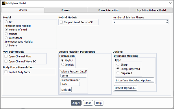
Number of Eulerian Phases
(optional) Coupled Level Set + VOF (see Coupled Level-Set and VOF Model in the Theory Guide)
volume fraction Formulation (Explicit or Implicit) and associated parameters (see Choosing Volume Fraction Formulation)
(optional) inclusion of sub-models such as and Open Channel Wave BC
Interface Modeling type and options (see Choosing Volume Fraction Formulation)
(optional) selection of Expert Options (see Expert Options)
(optional) inclusion of the Implicit Body Force formulation (see Including Body Forces)
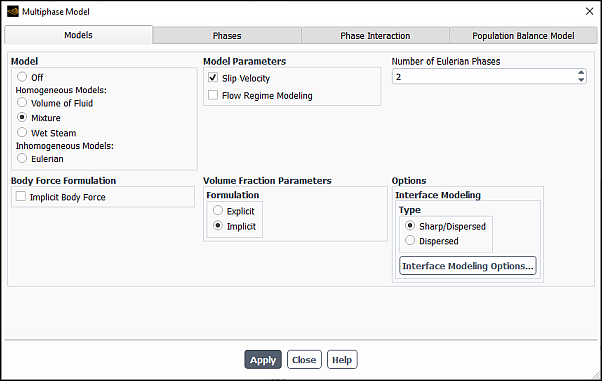
Number of Eulerian Phases
(optional) inclusion of Slip Velocity (see Solving a Homogeneous Multiphase Flow)
volume fraction Formulation (Explicit or Implicit) and associated parameters (see Choosing Volume Fraction Formulation)
Interface Modeling type and options (see Choosing Volume Fraction Formulation)
(optional) selection of Expert Options (see Expert Options)
(optional) inclusion of the Implicit Body Force formulation (see Including Body Forces)
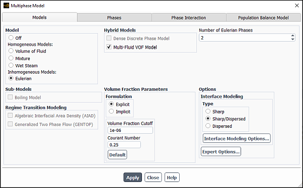
Number of Eulerian Phases
(optional) inclusion of the Dense Discrete Phase Model
(optional) inclusion of the Boiling Model
(optional) inclusion of the Multi-Fluid VOF Model
volume fraction Formulation (Explicit or Implicit) and associated parameters (see Choosing Volume Fraction Formulation)
Interface Modeling type and options (see Choosing Volume Fraction Formulation). This is only available if the Multi-Fluid VOF Model is enabled.
(optional) selection of Expert Options (see Expert Options)
To specify the number of phases for the multiphase calculation, enter the appropriate value in the Number of Eulerian Phases field. You can specify up to 20 phases.
Ansys Fluent supports the following options for volume fraction formulation:
- Explicit Formulation
The explicit formulation is non-iterative and is time-dependent. Thus it can only be used with the Transient solver. It exhibits better numerical accuracy compared to the implicit formulation. However the time step size is limited by a Courant-based stability criterion.
- Implicit Formulation
The implicit formulation is iterative and can be used with either the Steady or Transient solver. It is well-suited to steady-state applications as the solution information propagates much faster compared to the explicit formulation.
For steady-state flow applications, either a steady-state or a transient simulation may be required, depending on the characteristics of the flow:
Steady-state simulation: If the final steady-state solution is not affected by the initial flow conditions and there is a distinct inflow boundary for each phase.
Transient simulation: If the final steady-state solution is dependent on the initial flow conditions and/or you do not have a distinct inflow boundary for each phase.
For transient flow applications, the implicit formulation may allow you to use a much larger time step size than the explicit formulation due to the implicit formulation’s unconditional stability. However, the implicit time-step size may be limited by truncation errors. The implicit formulation produces more numerical diffusion than the explicit formulation when using the First Order transient formulation. Therefore, the implicit formulation should be used along with higher-order transient formulations to achieve better numerical accuracy.
To specify the volume fraction formulation to be used for the VOF and Eulerian multiphase models, select the appropriate Formulation under Volume Fraction Parameters in the Models tab of the Multiphase Model dialog box.
For the VOF and Mixture multiphase models and for the Eulerian multiphase model with Multi-Fluid VOF enabled, you must specify the interface regime that you will be modeling. This will determine the availability of the various volume fraction discretization schemes (Spatial Discretization Schemes for Volume Fraction). The following options are available for Interface Modeling Type:
- Sharp
(VOF and Multi-Fluid VOF models only) for when a distinct interface is present between the phases
- Dispersed
for when the phases are interpenetrating
- Sharp/Dispersed
a hybrid approach for flows consisting of both sharp and dispersed interfaces. This option can also be used to capture mildly sharp interfaces. Mildly sharp interfaces are those that are neither as sharp as would be captured by the schemes available with the Sharp option, nor as diffused as would be captured by the schemes available with the Dispersed option.
Interfacial Anti-Diffusion
If you are using the Sharp interface modeling type, you can optionally enable the Interfacial Anti-Diffusion treatment. This treatment is applied only in interfacial cells and attempts to suppress the numerical diffusion that can arise from the volume fraction advection schemes.
The use of this treatment can have adverse effects on convergence, especially with aggressive settings and large time step size. Therefore, it should be used in cases that use a coarse mesh, that have high aspect-ratio cells, that have large cell-volume jumps in the vicinity of the fluid-fluid interface, or that suffer from excess numerical diffusion.
The strength of the anti-diffusion treatment can be specified
using the define/models/multiphase/interface-modeling-options text command. The strength can range between 0 (none) and 1 (maximum).
The anti-diffusion treatment can sometimes produce artificial waves due to excessive sharpening. The dynamic anti-diffusion strength option may help in such cases by reducing the anti-diffusion strength in the direction tangential to the interface. Dynamic strength can be enabled using the following text commands.
solve/set/multiphase-numerics/advanced-stability-controls/anti-diffusion/enable-dynamic-strength?solve/set/multiphase-numerics/advanced-stability-controls/anti-diffusion/enable-dynamic-strength?Enable anti-diffusion treatment with dynamic strength? [no]yes
Dynamic strength is specified as:
 | (26–1) |
where
 = anti diffusion strength = anti diffusion strength |
 = interface unit normal = interface unit normal |
 = area unit normal = area unit normal |
 = angle between the area and interface unit normals = angle between the area and interface unit normals |
 = exponent (default = 1.5) = exponent (default = 1.5) |
 = maximum value of anti-diffusion strength ranging between 0 and 0.95
(default = 0.75) = maximum value of anti-diffusion strength ranging between 0 and 0.95
(default = 0.75) |
Values of the exponent and maximum strength can be adjusted using the following text commands, if needed:
-
solve/set/multiphase-numerics/advanced-stability-controls/anti-diffusion/set-dynamic-strength-exponent Sets the cosine exponent in the dynamic strength treatment (
 in Equation 26–1).
-
solve/set/multiphase-numerics/advanced-stability-controls/anti-diffusion/set-maximum-dynamic-strength Sets the maximum value of dynamic anti-diffusion strength (
 in Equation 26–1).
Sharp/Dispersed Interface Modeling Options
Selecting will make available some additional discretization options. To access these, click Interface Modeling Options... in the Multiphase Model dialog box.
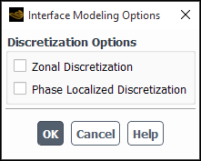
These options allow you to adjust the discretization behavior on a per-zone and/or per-phase-pair basis for cases in which it is important to simultaneously model dispersed and sharp interfaces.
- Zonal Discretization
This option is appropriate for applications that require either sharp or dispersed interface modeling depending on the cell zone. After enabling Zonal Discretization you will need to specify the slope limiter value on the Multiphase tab of the Fluid dialog box for each cell zone. (See Defining Multiphase Cell Zone and Boundary Conditions)
- Phase Localized Discretization
This option is appropriate for applications that require either sharp or dispersed interface modeling depending on the phase-pair comprising the interface. After enabling Phase Localized Discretization you will need to specify the slope limiter values for each phase pair in the Phase Interaction > Discretization tab of the Multiphase Model dialog box.
You can choose from various spatial discretization schemes for volume fraction depending on the multiphase model in use, the interface regime type, and the volume fraction formulation chosen. The available discretization schemes for each combination of model, formulation, and interface regime are summarized in the following tables:
Table 26.1: Spatial Discretization Schemes for the VOF and Eulerian with Multi-Fluid VOF Models
| Interface Modeling Type | Implicit Formulation | Explicit Formulation |
|---|---|---|
| Sharp |
Compressive |
Geo-Reconstruct |
| Sharp/Dispersed |
Compressive | |
| Dispersed |
First Order Upwind |
First Order Upwind |
Table 26.2: Spatial Discretization Schemes for the Eulerian Model without Multi-Fluid VOF
| Implicit Formulation | Explicit Formulation |
|---|---|
|
First Order Upwind |
First Order Upwind |
Table 26.3: Spatial Discretization Schemes for the Mixture Model
| Interface Modeling Type | Implicit Formulation | Explicit Formulation |
|---|---|---|
| Sharp/Dispersed |
Compressive | |
| Dispersed |
First Order Upwind | |
The Geo-Reconstruct scheme is an interface tracking scheme based on geometrical information. It is the most accurate scheme, but is more computationally expensive than the other schemes. Geo-Reconstruct is the preferred scheme when solving on meshes of poor quality.
The CICSAM, Modified HRIC, and Compressive schemes are interface capturing schemes based on algebraic information.
The Donor-Acceptor discretization is a scheme applicable only to quad- and hex-meshes. As it
is considered obsolete, it does not appear by default in the graphical user interface.
However, it can be made available if required using the following text command:
solve/set/advanced/show-all-discretization-schemes. This
command can also be used to expose discretization schemes that may be applicable, but are
hidden by default according to the tables above.
Important: For the geometric reconstruction and donor-acceptor schemes, if you are using a conformal mesh (that is, if the mesh node locations are identical at the boundaries where two subdomains meet), you must ensure that there are no two-sided (zero-thickness) walls within the domain. If there are, you will need to slit them, as described in Slitting Face Zones.
For more details about the implementations of the volume fraction discretization schemes, refer to Interpolation Near the Interface in the Fluent Theory Guide.
The Volume Fraction Cutoff allows you to specify a cutoff limit for the volume fraction values. The value that you provide is used as the lower cutoff for the volume fraction. All volume fraction values in the domain below this cutoff value are set to zero. The upper cutoff is calculated as (1.0 - lower cutoff). All volume fraction values above the upper cutoff value are set to 1.0. The default value is 1e-6, which is the recommended value. Using a higher value may lead to a higher volume imbalance.
Important: The Volume Fraction Cutoff value can be specified only with the Explicit formulation for volume fraction.
Note: For the Implicit formulation, the minimum value allowed is 0 and the maximum allowable value is 1e-6. For the Explicit formulation, the minimum value allowed is 0 and the maximum allowable value is 1e-4. A higher cutoff value is available with the Explicit formulation because it allows for the local redistribution procedure of partially filled cells, which accounts for volume loss. This treatment is not available with the Implicit formulation.
When using the Explicit formulation, there are several additional options that you can access in the Expert Options dialog box that opens by clicking Expert Options... in the Multiphase Model dialog box (Models tab).
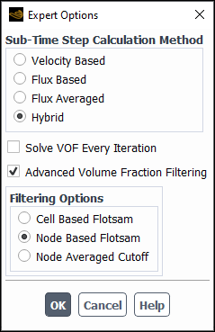
- Sub-Time Step Calculation Method
This setting controls how the time-scale is computed when determining the time step used for volume fraction.
- Solve VOF Every Iteration
This setting controls whether to solve the volume fraction equations once per iteration, or only once per time step.
For a more detailed discussion of how to use these options, refer to Setting Time-Dependent Parameters for the Explicit Volume Fraction Formulation.
In addition, you can enable Advanced Volume Fraction Filtering if you want to filter out small values of the volume fraction, which may be purely numerical causing solution instability. Small-scale numerical errors in the volume fraction field may arise due to the various reasons:
Time truncation errors at large time step size
Insufficient number of sub-time integration steps
Limiting and normalization of the volume fraction field
Ansys Fluent uses the flotsam filtering method to identify whether these errors are physical or numerical. The method is based on a principle that an interface cannot be constructed in a single cell.
Figure 26.5: Numerical Flotsams in the Volume Fraction Field depicts generation of a numerical flotsam. In scenario A, the neighboring cells are completely full, while the central cell is not full. In scenario B, the neighboring cells are completely void, but the central cell contains a non-zero volume fraction. Both scenarios cannot exist unless there is a mass source/sink present in a single cell.
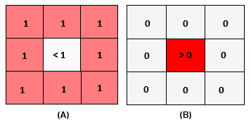
Once a cell is identified as a flotsam, its volume fraction is removed from the cell and distributed to the partial cells (that is, cells with the volume fraction between 0 and 1).
You can select one of the following Filtering Options:
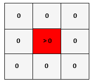
- Cell Based Flotsam
Flotsams are identified using only face-connected neighbors (see Figure 26.6: The Volume Fraction Field for the Cell Based Flotsam Detection). This method is rather aggressive, and there is a possibility of filtering out a ligament that passes through a central cell diagonally (in both scenarios A and B shown in Figure 26.5: Numerical Flotsams in the Volume Fraction Field).
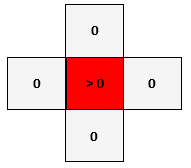
- Node Based Flotsam
Flotsams are identified using node-connected neighbors (see Figure 26.7: The Volume Fraction Field for the Node Based Flotsam Detection). This method is quite conservative, and there is no possibility of filtering out a ligament that passes a central cell diagonally (in both scenarios A and B shown in Figure 26.5: Numerical Flotsams in the Volume Fraction Field).
- Node Averaged Filtering Method
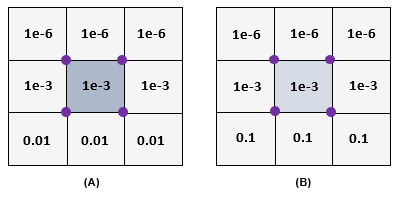
This method filters out the volume fraction in a cell when the node-averaged volume fraction in the cell falls below a specified cutoff value.
For example, Figure 26.8: The Volume Fraction Field for the Node-Averaged Filtering shows different scenarios for a cutoff value of 0.01. In the left-hand side (A), the central cell qualifies for the filtering criterion because the node-averaged value in the central cell is below 0.01; and therefore, the volume fraction will be removed from the cell and distributed in the neighboring cells. In the right-hand side (B), the central cell does not fall under the cutoff criterion, so its volume fraction will remain intact.
If you select this method, you can adjust the Volume Fraction Filtering Cutoff. The default value is 0.001.
If you are using the mixture model, you have the option to disable the calculation of slip velocities and solve a homogeneous multiphase flow (that is, one in which the phases all move at the same velocity). By default, Ansys Fluent will compute the slip velocities for the secondary phases, as described in Relative (Slip) Velocity and the Drift Velocity in the Theory Guide. If you want to solve a homogeneous multiphase flow, turn off Slip Velocity under Mixture Parameters.
Ansys Fluent provides the following methods for calculation of operating density for a buoyancy-driven flow. These options appear in the Operating Density drop-down list in the Operating Conditions dialog box (Variable-Density Parameters group box).
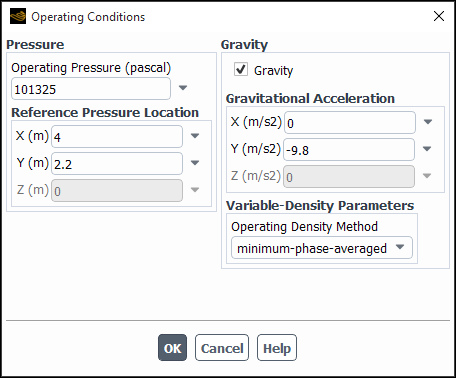
minimum-phase-averaged: ( default) Operating density is taken as the minimum of averaged densities calculated for each phase. For a compressible flow, operating density is internally set to zero.
primary-phase-averaged: Operating density is taken as the averaged density of the primary phase.
mixture-averaged: Operating density is taken as the averaged density of the mixture in the whole domain.
user-input: Allows you to provide your own values for specific needs.
The default method, minimum-phase-averaged, is appropriate for most cases, and typically you do not need to change it. It automatically handles the operating density requirements for both incompressible and compressible flows by resolving the correct hydrostatic pressure gradient distribution.
If you are interested only in the pressure gradient (rather than the hydrostatic pressure values), you can use either the primary-phase-averaged or mixture-averaged method.
When using the Boussinesq approximation for density variation in multiphase flows, there are several important items to consider:
The Boussinesq approximation is only valid for small variations in fluid densities caused by small variations in temperature. Therefore, constant density is assumed, and a momentum source is only added for modeling buoyancy.
The Boussinesq approximation assumes that small density variations have little effect on inertial terms and strong effects on gravitational terms. Thus, the differences in specific weights between two fluids or layers of fluids is the force driving the flow. (Waves cannot use this approximation.) Two non-dimensional numbers quantify the effect of buoyancy: the Richardson number and the Rayleigh number.
Operating density should be set to zero.
For additional information on the Boussinesq approximation, see The Boussinesq Model.
If you are using any of the multiphase models for a compressible flow, note the following:
Ansys Fluent allows the modeling of:
Multiple compressible ideal gas phases and/or incompressible/compressible liquids at any inlet
A single real gas or real liquid at any inlet
Multiple real gases at a single inlet
Multiple compressible liquids using either the Fluent built-in compressible liquid density model based on the Tait law (see Compressible Liquid Density Method) or user-defined functions
For multiple compressible phases, the fundamental equations for compressible flow remain the same. However, boundary conditions are modified to account for changes in material properties due to compressible fluid mixtures.
In cases of a mixture of ideal and real gases, the phases must enter the domain through separate inlets.
When using the VOF model, stability is improved if the primary phase is the compressible ideal gas.
If you specify the total pressure at a boundary (for example, for a pressure inlet or intake fan), Fluent will use the specified value for temperature at that boundary as total temperature for the compressible phase, and as static temperature for the other phases (which are incompressible).
For each mass-flow inlet, you will need to specify mass flow or mass flux for each individual phase.
Important: Note that if you read a case file that was set up in a version of Fluent previous to 6.1, you will need to redefine the conditions at the mass-flow inlets. See Defining Multiphase Cell Zone and Boundary Conditions for more information on defining conditions for a mass-flow inlet in multiphase calculations.
Enhanced Compressible Flow Numerics
Compressible flow simulations may have convergence difficulties due to explicit handling of source term accounting for density variation. These simulations could become extremely unstable in the presence of a large variation in pressure and temperature. In Ansys Fluent, an enhanced numerical treatment that provides better stability at startup and during calculation of compressible flows is enabled by default. The treatment controls the rate of change of pressure and temperature between iterations and provides additional diagonal dominance to the matrix of equations.
Although disabling the enhanced numerical treatment is not recommended, you can temporarily turn it off to investigate unstable cases using the following text user interface command:
solve/set/multiphase-numerics/compressible-flow/enhanced-numerics
...
enhanced compressible flow numerics? [yes] no
See Compressible Flows for more information about compressible flows.
Alternative Compressible Flow Numerics
A more general formulation for compressible multiphase flows employs a mathematically rigorous treatment of compressible phases at an inlet boundary. Instead of treating the entering incompressible and compressible phases as a pseudo-mixture, this formulation calculates static temperature and pressure using an iterative method based on fundamental thermodynamic relations (such as the Maxwell relations). This approach involves evaluation of the property derivatives, which can be computed either numerically or through analytic expressions. You can enable this alternative treatment via the text command:
solve/set/multiphase-numerics/compressible-flow/alternate-bc-formulation alternate compressible bc formulation? [no]yuse analytical thermodynamic derivatives? [no]y
You can define the phases (including their material properties) in the Phases tab of the Multiphase Model dialog box (Figure 26.10: The Multiphase Model dialog box - Phases tab).
![]() Setup
→ Models → Multiphase
Setup
→ Models → Multiphase![]() Edit...
Edit...

Each item in the Phases list is one of two types:
A Primary-Phase indicates that the selected item is the primary phase.
A Secondary-Phase indicates that the selected item is a secondary phase.
In the Phase Setup group box, you can specify the name of the phase (19 characters maximum) and select its material.
You can specify any interaction between the phases (for example, surface tension and wall adhesion for the VOF model, slip velocity for the mixture model, drag functions for the mixture and the Eulerian models) in the Phase Interaction tab of the Multiphase Model dialog box.
Instructions for defining mass transfer between phases can be found in Including Mass Transfer Effects.
Instructions for defining heterogeneous reactions for species transport cases are provided in Specifying Heterogeneous Reactions.
Instructions for defining the phases and model-specific phase interactions are provided in the following sections:
VOF model: Defining the Phases for the VOF Model
Mixture model: Defining the Phases for the Mixture Model
Eulerian model: Defining the Phases for the Eulerian Model
When large body forces (for example, gravity or surface tension forces) exist in multiphase flows, the body force and pressure gradient terms in the momentum equation are almost in equilibrium while the contributions of convective and viscous terms are small in comparison. Segregated algorithms converge poorly unless partial equilibrium of pressure gradient and body forces is taken into account. Ansys Fluent provides an optional “implicit body force” treatment that can account for this effect, making the solution more robust.
The basic procedure involves augmenting the correction equation for the face flow rate, Equation 23–56 in the Theory Guide, with an additional term involving corrections to the body force. This results in extra body force correction terms in Equation 23–54 in the Theory Guide, and allows the flow to achieve a realistic pressure field very early in the iterative process.
To include this body force, enable Gravity in the Operating Conditions Dialog Box and specify the Gravitational Acceleration.
![]() Setup →
Setup → ![]() Cell Zone Conditions → Operating Conditions...
Cell Zone Conditions → Operating Conditions...
For VOF calculations, you should also enable the Specified Operating Density option in the Operating Conditions dialog box, and set the Operating Density to be the density of the lightest phase. (This excludes the buildup of hydrostatic pressure within the lightest phase, improving the round-off accuracy for the momentum balance.) If any of the phases is compressible, set the Operating Density to zero.
Important: For VOF and mixture calculations involving body forces, it is recommended that you also enable the Implicit Body Force treatment for the Body Force Formulation in the Multiphase Model dialog box. This treatment improves solution convergence by accounting for the partial equilibrium of the pressure gradient and body forces in the momentum equations. See Including Body Forces for details.
In Ansys Fluent , you can set up a multiphase species transport and volumetric reaction (Modeling Species Transport in Multiphase Flows in the Theory Guide) in a fashion that is similar to setting up a single-phase chemical reaction using the Species Model dialog box (for example, Figure 26.11: The Species Model Dialog Box with a Multiphase Model Enabled).
Note: Note that the Full Multicomponent Diffusion option in the Species Model dialog box (Options group), in not used when modeling multiphase species transport. Instead, you can enable the Full Multicomponent Diffusion option for a selected phase in the Phase Properties dialog box as further described.
![]() Setup →
Setup → ![]() Models →
Models → ![]() Species → Edit...
Species → Edit...
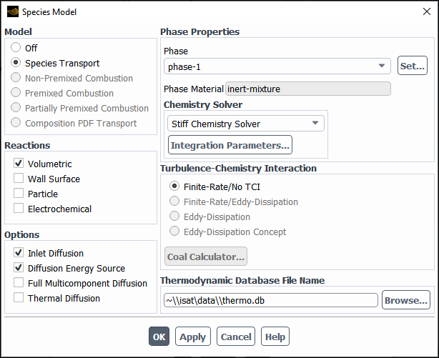
Select Species Transport under Model.
Enable Volumetric under Reactions.
If you have already enabled a multiphase model, then you need to select a multi-species phase and assign to it a mixture material. By default, the primary phase is selected in the Phase drop-down list, and the fluid material assigned to it is displayed in the Phase Material information box (Phase Properties group box).
In the Phase drop-down list, select a phase for a species mixture material.
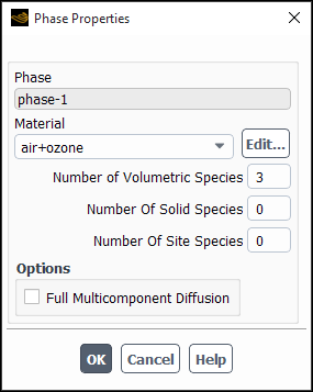
Click the button to display the Phase Properties dialog box (see Figure 26.12: The Phase Properties Dialog Box).
In the Material drop-down list, the materials for each phase already defined in your case are listed at the top followed by the mixture materials from the Fluent database materials. From this list, choose the material that you want to use for a multi-species phase.
If you want to use the full multicomponent diffusion model described in Full Multicomponent Diffusion in the Fluent Theory Guide for the selected phase, enable the Full Multicomponent Diffusion option.
Click to close the Phase Properties dialog box.
(Eulerian multiphase model only) In the Species Model dialog box, select the solver for your simulation from the Chemistry Solver drop-down list.
If you want to solve finite-rate chemistry, select the Stiff Chemistry Solver.
Note: The Stiff Chemistry Solver can be used only for one mixture-material phase.
If you want to make explicit use of chemistry source terms in the phase-specific species transport equations, without a stiff-chemistry solver, select None – Explicit Source. Note that this solver is not recommended for stiff or complex chemistry.
(optional) If you selected Stiff Chemistry Solver in the previous step, then in the Integration Parameters Dialog Box (opened by clicking the Integration Parameters... button), you can:
adjust the ODE Parameters
enable the ISAT integration method to accelerate chemistry calculations and set up its parameters. See Using ISAT for additional information.
In the Species Model dialog box, choose the Turbulence-Chemistry Interaction model. Three models are available:
- Finite-Rate/No TCI
computes only the Arrhenius rate (see Equation 7–21 in the Theory Guide) and neglects turbulence-chemistry interaction.
- Finite-Rate/Eddy-Dissipation
(for turbulent flows) computes both the Arrhenius rate and the mixing rate and uses the smaller of the two.
Click in the Species Model dialog box.
Once you click , the mixture material you selected for the multi-species phase will be copied to your case and appear under the Setup/Materials/Mixture tree node in the Outline View.
When modeling multiphase species transport, additional inputs may also be required depending on your modeling needs. See, for example, Specifying Heterogeneous Reactions for more information defining heterogeneous reactions, or Including Mass Transfer Effects for more information on mass transfer effects.
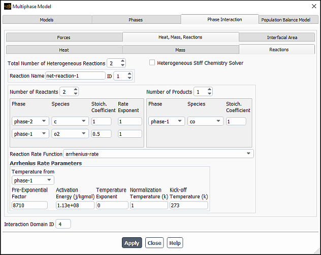
You can define multiple heterogeneous reactions and stoichiometry in the Reactions tab of the Multiphase Model dialog box (for example, Figure 26.13: The Reactions Tab for Heterogeneous Reactions).
![]() Setup → Models →
Multiphase
Setup → Models →
Multiphase ![]() Edit...
Edit...
In the Multiphase Model dialog box (Figure 26.10: The Multiphase Model dialog box - Phases tab), go to the Phase Interaction > Heat, Mass, Reactions > Reactions tab.
Set the total number of reactions (volumetric reactions, wall surface reactions, and particle surface reactions) in the Total Number of Heterogeneous Reactions field. (Use the arrows to change the value, or type in the value and press Enter.)
Enable the Heterogeneous Stiff Chemistry Solver option if your interphase reaction mechanism contains numerically stiff reactions. This option can improve convergence and is available for transient Eulerian multiphase simulations. When this option is enabled, Ansys Fluent uses a fractional step algorithm where the flow is advanced without reaction sources for a time step, and then the chemistry is integrated point-by-point for the same time step. The stiff chemistry scheme solves all species in all phases coupled. Note that it is possible to include homogeneous (intra-phase) reactions along with the heterogeneous reactions in the Reactions tab (instead of in the reaction mechanism in the Create/Edit Materials dialog box), and these reactions will be solved with the stiff solver. The stiff ODE solver tolerances can be set using the following text command:
solve→set→heterogeneous-stiff-chemistrySpecify the Reaction Name of each reaction that you want to define.
Set the ID of each reaction you want to define. (Again, if you type in the value be sure to press Enter.)
For each reaction, specify how many reactants and products are involved in the reaction by increasing the value of the Number of Reactants and the Number of Products. Select each reactant or product in the Reaction tab and then set its stoichiometric coefficient in the Stoich. Coefficient field. (The stoichiometric coefficient is the constant
 or
or  in Equation 7–20 in the Theory Guide.)
For each reaction, indicate the Phase and Species and the stoichiometric coefficient for each of your reactants and products.
For each reaction, use the Reaction Rate Function drop-down list to select one of the following:
- none
if you do not want to include a reaction rate
- population-balance
is the mass transfer due to nucleation and growth. If neither the primary phase or secondary phase has species associated with it, then the mass transfer is modeled as unidirectional. If the mass transfer process involves reactions or species, the problem must be set up as one involving heterogeneous reaction/mass transfer.
Important: The population-balance option for Reaction Rate Function should not be used if there are multiple reactions leading to the formation of the secondary phase. In this case, the reaction rate functions should be specified either through the standard dialog boxes or user-defined functions and the growth rate function should be a sum of the individual reaction rates. This would ensure consistency between the individual reaction rates and the total mass transfer from the primary to the secondary phase.
You can always use
DEFINE_MASS_TRANSFERorDEFINE_HET_RXN_RATEuser-defined function types instead of the population-balance option to specify mass transfer rates. However, the growth rate function and the mass transfer rates returned from the UDFs need to be consistent with each other.- arrhenius-rate
to specify rate exponents for an Arrhenius-type reaction (see Heterogeneous Phase Interaction in the Theory Guide for more information)
Important: This simple form of the Arrhenius rate option may only be used for devolatilization reactions only. Char combustion reaction may be more involved and complicated to be simply casted in this form. Additional diffusion rate formulations may be needed to formulate a complete char (or solid phase) reaction system.
Important: Note that you can also specify the heterogeneous reaction rates using a user-defined function. A user-defined function is available for an Arrhenius-type reaction with rate exponents that are equivalent to the stoichiometric coefficients. For more information, see
DEFINE_HET_RXN_RATEin the Fluent Customization Manual.Click Apply.
Important: Ansys Fluent assumes that the reactants are mixed thoroughly before reacting together, therefore the heat and momentum transfer is based on this assumption. This assumption can be disabled using a text command. For more information, contact your Ansys Fluent support engineer.
As discussed in Modeling Mass Transfer in Multiphase Flows in the Theory Guide, mass transfer effects in the framework of Ansys Fluent’s general multiphase models (that is, Eulerian multiphase, mixture multiphase, or VOF multiphase) can be modeled in one of three ways:
Unidirectional constant rate mass transfer
UDF-prescribed mass transfer
mass transfer through cavitation, evaporation-condensation, boiling, or generalized species mass transfer
Note: For limitations regarding the cavitation models, see Limitations of the Cavitation Models in the Fluent Theory Guide.
You can define mass transfer in a multiphase simulation as a unidirectional constant, using a user-defined function, through population balance, cavitation, evaporation/condensation, or species mass transfer. To do this, go to the Phase Interaction > Heat, Mass, Reactions > Mass tab in the Multiphase Model dialog box.
![]() Setup → Models →
Multiphase
Setup → Models →
Multiphase ![]() Edit...
Edit...
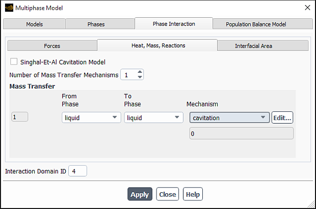
Specify the Number of Mass Transfer Mechanisms.
Important: In general, you should use only one mass transfer mechanism when you employ one of the available mass transfer models (see Step 7). Although using multiple mass transfer mechanisms is allowed for any pairs of phases (including the same pair of phases), it is not recommended because the mass transfer models have been fundamentally developed for a single mass transfer process. These models do not account for possible interactions between two mass transfer mechanisms in a flow system. In order to account for all relevant physics using UDFs in multiple mass transfer mechanisms, you can use the user-defined option. For additional restrictions when using multiple mass transfer mechanisms, see Step 7.
For each mechanism, specify the phase of the source material under From Phase. Note that the phase you select for From Phase must be a liquid if you plan to select cavitation, evaporation-condensation, or boiling from the Mechanism drop-down menu (see Step 7).
If species transport is part of the simulation, and the source phase is composed of a mixture material, then specify the species of the source phase mixture material in the corresponding Species drop-down list.
For each mechanism, specify the phase of the destination material phase under To Phase. Note that the phase you select for To Phase must be a vapor if you plan to select cavitation, evaporation-condensation, or boiling from the Mechanism drop-down menu. If you plan to select species-mass-transfer and one of the phases is a gas, it must be specified as the To Phase (see Step 7).
If species transport is part of the simulation, and the destination phase is composed of a mixture material, then specify the species of the destination phase mixture material in the corresponding Species drop-down list.
For each pair of phases with mass transfer, select the desired mass transfer mechanism under Mechanism. The available mechanisms and their inputs are described in Mass Transfer Mechanisms.
Ansys Fluent will automatically include the terms needed to model mass transfer in all relevant conservation equations. Another option to model mass transfer between phases is through the use of user-defined sources and their inclusion in the relevant conservation equations. This approach is more involved, but more powerful, allowing you to split the source terms according to a model of your choice.
Click Apply.
Important:
Except for the species-mass-transfer mechanism, if the same mass transfer model is selected for multiple mass transfer mechanisms, the most recently edited mechanism sub-model, including its parameters, options, and constants (excluding its material properties, such as vaporization pressure or saturation temperature), will apply to all the mass transfer mechanisms.
When modeling multiple species-mass-transfer mechanisms, you can select different species mass transfer models and model options, such as Raoult's Law, Henry's Law, etc. However, because there is a lack of interaction between different species mass transfer models, this should be done with caution. For information on modeling restrictions for interphase species mass transfer, see Interphase Species Mass Transfer in the Fluent Theory Guide.
Momentum, energy, and turbulence are also transported with the mass that is transferred. Ansys Fluent assumes that the reactants are mixed thoroughly before reacting together, therefore the heat and momentum transfer is based on this assumption. This assumption can be disabled using a text command. For more information, contact your Ansys Fluent support engineer.
When your model involves the transport of multiphase species, you can define a mass transfer mechanism between species from different phases. If a particular phase does not have a species associated with it, then the mass transfer throughout the system will be performed by the bulk fluid material.
Important: Including species transport effects in the mass transport of multiphase simulation requires that Species Transport be selected in the Species Model dialog box.
![]() Setup →
Setup → ![]() Models →
Models → ![]() Species
Species
The existing formulation of sensible enthalpy for interphase mass transfer includes the formation enthalpy, which could be problematic for some cases, such as cases that involve species transport and reactions. The alternative treatment, which is available with the VOF and Mixture multiphase models, is based on the explicit modeling of the energy source driven by mass transfer. You can enable the alternative formulation by using the following text command:
solve/set/multiphase-numerics/heat-mass-transfer/alternative-energy-treatment?
enable alternative treatment of handling latent heat source [no]
              y
Energy Source Treatment
The energy source is modeled explicitly as:
 | (26–2) |
where  is the mass transfer rate, and
  is latent heat of vaporization. If you are using the
tabular-ptl-sat method to specify saturation temperature for the
Evaporation-Condensation Mechanism or vaporization pressure for the
Cavitation Mechanism, Ansys Fluent will take the latent heat
values directly from the tabular data. Otherwise, it is calculated as:
is latent heat of vaporization. If you are using the
tabular-ptl-sat method to specify saturation temperature for the
Evaporation-Condensation Mechanism or vaporization pressure for the
Cavitation Mechanism, Ansys Fluent will take the latent heat
values directly from the tabular data. Otherwise, it is calculated as:
 | (26–3) |
Here,  and
and  are saturation enthalpies of phase
  and phase
  at the saturation temperature, respectively. They are calculated
as:
at the saturation temperature, respectively. They are calculated
as:
 | (26–4) |
 | (26–5) |
| where, | |
 and and  = formation enthalpies of phase = formation enthalpies of phase  and phase and phase  , respectively , respectively | |
 and and  = specific heats of phase and phase , respectively = specific heats of phase and phase , respectively | |
 and and  = reference temperatures of phase and phase as specified in the Create/Edit Materials
dialog box, respectively. = reference temperatures of phase and phase as specified in the Create/Edit Materials
dialog box, respectively. | |
 = saturation temperature = saturation temperature |
Note: For mass transfer mechanisms that do not require explicit input of saturation temperature, such as cavitation and species mass transfer, the saturation temperature is assumed as the reference temperature of the liquid.
Sensible Enthalpy Definition
For mass transfer cases, Ansys Fluent by default uses the following definition of sensible enthalpy:
 | (26–6) |
| where, | |
 = sensible enthalpy of phase = sensible enthalpy of phase
| |
 = formation enthalpy of phase = formation enthalpy of phase
| |
 = specific heat of phase = specific heat of phase
| |
 = temperature of phase = temperature of phase
| |
 = reference temperature of phase as specified in the Create/Edit Materials
dialog box = reference temperature of phase as specified in the Create/Edit Materials
dialog box |
The alternative treatment considers the definition of sensible enthalpy that excludes formation enthalpy. Sensible enthalpy for each phase is expressed as:
 | (26–7) |
with  =298.15 K.
Heat Flux Reporting Strategies
When you use the alternative formulation, the following additional variable become available for postprocessing under the Phase Interaction... category:
Latent Heat
In the variable selection drop-down lists that appear in postprocessing dialog boxes, this quantity will be appended with the ID of the corresponding mass transfer mechanism.
Due to the explicit nature of the alternative formulation, the latent heat source appears as the heat imbalance in heat flux reporting.
If you want to know the heat imbalance due to the latent heat source, you should create a custom-field function for the mass transfer rate multiplied by latent heat, and then report it as a volume integral. Ansys Fluent will report the following value:
 | (26–8) |
| where, | |
 = heat imbalance = heat imbalance | |
 = number of mass transfer mechanisms that you defined = number of mass transfer mechanisms that you defined | |
 = mass transfer rate of = mass transfer rate of  th mechanism
 | |
 = Latent heat of = Latent heat of  th mechanism
 | |
 = volume = volume |
When including mass transfer effects in a multiphase simulation, you can choose from the following mechanisms for each phase pair that undergoes mass transfer:
constant-rate
user-defined
population-balance
cavitation
evaporation-condensation
species-mass-transfer
boiling
Details for each mechanism are provided in the following sections:
You can use the constant-rate option to specify a constant value for unidirectional mass transfer. The constant-rate must be entered in units of 1/time unit.
The user-defined option allows you to implement a correlation reflecting a model of your choice, through a user-defined function.
With the population-balance mechanism, you can model flow where a number density function is introduced to account for the particle population. With the aid of particle properties (for example, particle size, porosity, composition, and so on), different particles in the population can be distinguished and their behavior can be described. For a comprehensive understanding of this option, refer to Population Balance Model .
The cavitation mechanism allows you to select a cavitation model. For a cavitating flow, it is recommended that you select liquid as the primary phase and vapor as the secondary phase.
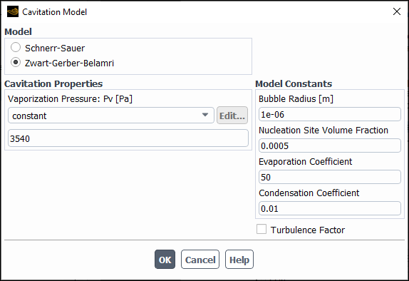
The cavitation models are available when using mixture, VOF, and Eulerian multiphase models. You are provided with two model options: Schnerr-Sauer and Zwart-Gerber-Belamri. To open the Cavitation Model dialog box, select cavitation from the Mechanism drop-down list. For information about the cavitation models, refer to Cavitation Models in the Theory Guide.
For the Schnerr-Sauer model, specify the Bubble Number Density (
 in Equation 14–588 in the Fluent Theory Guide)
under Model Constants. The default value of 1e11 is suitable
for most cases.
in Equation 14–588 in the Fluent Theory Guide)
under Model Constants. The default value of 1e11 is suitable
for most cases.For the Zwart-Gerber-Belamri model, specify the Bubble Radius, the Nucleation Site Volume Fraction, the Evaporation Coefficient, and the Condensation Coefficient under Model Constants.
Under Cavitation Properties, specify the Vaporization Pressure and, if desired, a temperature dependence function. In addition to the methods described in Defining Properties Using Temperature-Dependent Functions (constant, polynomial, piecewise-linear, piecewise-polynomial, or user-defined), you can choose one of the following:
rgp-table-sat
This option allows you to use to define the vaporization pressure using RGP tables as described in Defining Saturation Properties via RGP Tables.
taylor-approximation
The taylor-approximation method models the vaporization pressure as linearly varying with temperature about the free-stream value. This approach can improve numerical stability, but is only appropriate when deviations about the free-stream temperature are sufficiently small that higher-order terms can be neglected. The expression for the vaporization pressure using the taylor-approximation method is:

(26–9)
where
 is the free-stream temperature,
  is the latent heat, and
  is a user-modifiable coefficient. In the Taylor
Approximation dialog box, you will specify Vaporization
Pressure (at the free-stream temperature), Free Stream
Temperature, and Thermal Coefficient
(
is a user-modifiable coefficient. In the Taylor
Approximation dialog box, you will specify Vaporization
Pressure (at the free-stream temperature), Free Stream
Temperature, and Thermal Coefficient
( ).
).tabular-pt-sat
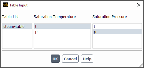
This method allows you to specify vaporization pressure using a table that contains data points for saturation temperature and saturation pressure. Saturation pressure will be interpolated based on the static temperature from the solution, which is assumed to be at a saturated state. The table format is described in Reading Files in Tabular Format. Once you select tabular-pt-sat, the Table Input dialog box opens where you can select the appropriate table and the names of the columns from the Saturation Temperature and Saturation Pressure selection lists.
tabular-ptl-sat
(available only with Alternative Modeling of Energy Sources) The method allows you to specify saturation pressure using a table that contains data points for saturation temperature, saturation pressure, and latent heat. Saturation pressure and latent heat will be interpolated based on the static temperature from the solution, which is assumed to be at a saturated state. The table format is described in Reading Files in Tabular Format. Once you select tabular-ptl-sat, the Table Input dialog box opens where you can select the appropriate table and the names of the columns from the Saturation Temperature, Saturation Pressure and Latent Heat selection lists.
Note: If you are using tabular-pt-sat or tabular-ptl-sat to specify vaporization pressure, you must first read an appropriate table following the procedure outlined in Reading Files in Tabular Format. All table data must be in SI units (saturation temperature in Kelvin (K), saturation pressure in Pascal (Pa), and latent heat in Joule/Kg).
If you want to include the influence of turbulence on the threshold cavitation pressure, enable Turbulence Factor. If desired, you can adjust the value of the Turbulent Coefficient. For details about the implementation of the Turbulence Factor, see Turbulence Factor in the Fluent Theory Guide.
By default, the minimum vapor pressure limit is set to 1 Pa. The default value for
the maximum vapor pressure limit is set to five times the local vapor pressure with
consideration of the turbulent and thermal effects for each computational cell and
phase. The default and recommended value for the evaporation and condensation
coefficients in the Schnerr-Sauer model ( and
and  in Equation 14–592 in the Fluent Theory Guide) are 1
and 0.2, respectively. You can modify these default values using the following expert
text commands:
in Equation 14–592 in the Fluent Theory Guide) are 1
and 0.2, respectively. You can modify these default values using the following expert
text commands:
solve/set/multiphase-numerics/heat-mass-transfer/cavitation/min-vapor-pressuresolve/set/multiphase-numerics/heat-mass-transfer/cavitation/max-vapor-pressure-ratiosolve/set/multiphase-numerics/heat-mass-transfer/cavitation/schnerr-cond-coeffsolve/set/multiphase-numerics/heat-mass-transfer/cavitation/schnerr-evap-coeff
Note:
If you use multiple cavitation mass transfer mechanisms in your simulation, the value you specify for Turbulence Factor will automatically apply to all cavitation mechanisms, thereby overwriting previously existing turbulent coefficients.
For the Mixture multiphase model, in addition to the Schnerr-Sauer and Zwart-Gerber-Belamri models, the Singhal et al. expert cavitation model can be used. See Using the Singhal et al. Expert Cavitation Model for more information on using this model.
Pressure Limiting Method
When calculating the properties of a compressible flow (such as densities and sound speeds), the cavitation model by default limits the absolute pressure to the vapor pressure whenever the absolute pressure drops below the vapor pressure. This default treatment may not predict correct results for a compressible flow because at saturation pressure, the density method behaves as the incompressible-ideal-gas law rather than the ideal-gas law. In such a case, you can apply a special treatment that allows the pressure to drop to the minimum absolute pressure. The treatment correctly predicts shock, which is not possible with the default treatment. To set the pressure limiting method, use the following text command:
solve/set/multiphase-numerics/heat-mass-transfer/cavitation/p-limit-method
The available methods are:
local-pvap-min: Limits the pressure to the local minimum of vapor pressuresglobal-pvap-min: Limits the pressure to the global minimum of vapor pressures from all cellspabs-min: Limits the pressure to the absolute minimum pressure specified under solution limits specified in the Solution Limits dialog box.
For a cavitating flow, by default, pressure contours are clipped to the pressure specified by the pressure limiting method wherever the pressure drops below the vapor pressure. To see the actual pressure contours, use the following text command:
solve/set/multiphase-numerics/heat-mass-transfer/cavitation/display_clipped_pressure?
display clipped pressure in the post-processing [yes]:
no
Note: Clipped pressure values are only used in the computation of properties, while the actual pressure, which is used in the calculation of the mass transfer rate, remains unclipped.
Turbulent Diffusion Treatment
For turbulent flows, if one of the phases participating in cavitation is primary, then Ansys Fluent automatically enables the generalized turbulent diffusion treatment. The treatment adds a diffusion source in the volume fraction equation by assuming the diffusion coefficient as a function of turbulent viscosity of the respective phase. This helps avoid instantaneous solution instability due to cavitation. For more information about this treatment, see Diffusion in VOF Model in the Fluent Theory Guide.
The generalized turbulent diffusion treatment can be used for simulating flows with two or more phases. By default, for a flow with more than two phases, the turbulent diffusion acts between primary and secondary phases only. The turbulent diffusion between secondary phases is not accounted for.
If you want to use the old turbulent diffusion treatment supported in releases prior to Release 19.2, enter the following text commands:
solve/set/multiphase-numerics/heat-mass-transfer/cavitation/turbulent-

diffusion
use generalized treatment of turbulent diffusion [yes] no
use old treatment of turbulent diffusion [yes] yes
Unlike the generalized turbulent diffusion treatment, the old treatment is applicable to only two-phase flows. If used for flows with more than two phases, the old treatment unphysically accounts for each secondary phase interacting with the primary phase, despite the secondary non-vapor phases not participating in cavitation.
If your want to disable the turbulent diffusion treatment for cases where the high turbulent viscosity may be a source of an unstable solution, enter the following text commands:
solve/set/multiphase-numerics/heat-mass-transfer/cavitation/turbulent-

diffusion
use generalized treatment of turbulent diffusion [yes] no
use old treatment of turbulent diffusion [yes] no
The evaporation-condensation mass transfer mechanism enables you to apply the evaporation-condensation model as the mass transfer mechanism. The VOF and Mixture multiphase models use the Lee model (see Lee Model in the Fluent Theory Guide). With the Eulerian multiphase model, you can choose between the Lee model and the Thermal Phase Change model (see Thermal Phase Change Model in the Fluent Theory Guide). When you select evaporation-condensation under Mechanism in the Phase Interaction > Heat, Mass, Reactions > Mass tab of the Multiphase Model dialog box, you will be prompted with the Evaporation-Condensation Model dialog box. Note that this dialog box could also be accessed by clicking Edit... next to the evaporation-condensation mechanism drop-down list.
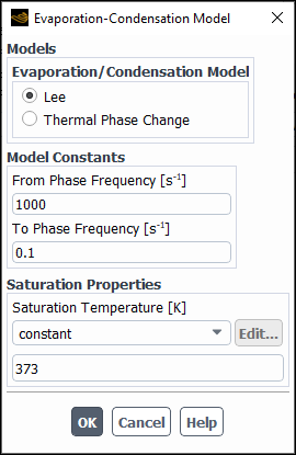
You need to specify the following settings:
(Eulerian multiphase model only) Select the evaporation-condensation Model. The following models are available:
Lee
Thermal Phase Change
Specify the Saturation Temperature for your flow regime. In addition to the methods described in Defining Properties Using Temperature-Dependent Functions (constant, polynomial, piecewise-linear, piecewise-polynomial, or user-defined) you can choose one of the following:
rgp-table-sat
This option allows you to use to define the saturated temperature using RGP tables as described in Defining Saturation Properties via RGP Tables.
tabular-pt-sat
The tabular-pt-sat allows you to specify saturation temperature using a table that contains data points for saturation temperature and saturation pressure. Saturation temperature will be interpolated based on the absolute pressure from the solution, which is assumed to be at a saturated state. The table format is described in Reading Files in Tabular Format. Once you select tabular-pt-sat, the Table Input dialog box opens where you can select the appropriate table and the names of the columns for your simulation from the Saturation Temperature and Saturation Pressure selection lists.
tabular-ptl-sat
(available only with Alternative Modeling of Energy Sources) The method allows you to specify saturation temperature using a table that contains data points for saturation temperature, saturation pressure, and latent heat. Saturation temperature and latent heat will be interpolated based on absolute pressure from the solution, which is assumed to be at a saturated state. The table format is described in Reading Files in Tabular Format. Once you select tabular-ptl-sat, the Table Input dialog box opens where you can select the appropriate table and the names of the columns from the Saturation Temperature, Saturation Pressure and Latent Heat selection lists.
Note:If you use tabular-pt-sat or tabular-ptl-sat to specify saturation temperature, you must first read an appropriate table following the procedure outlined in Reading Files in Tabular Format. All table data must be in SI units (saturation temperature in Kelvin (K), saturation pressure in Pascal (Pa), and latent heat in Joule/Kg).
If you use the tabular-pt-sat, tabular-ptl-sat, polynomial, piecewise-polynomial, or piecewise-linear option for Saturation Temperature, the pressure-dependency must be specified in terms of absolute pressure.
(Lee model only) Specify the From Phase Frequency and To Phase Frequency model constants. These values correspond to the coefficient
 (Equation 14–617 in the
Theory Guide). The values are
(Equation 14–617 in the
Theory Guide). The values are
0.1by default. However, note that the bubble diameter and accommodation coefficient are usually not very well known, so the appropriate values for a given problem can be very different. It is important to tune the values to match experimental data.(Mixture multiphase model only) For certain models and conditions, you can select the Semi-Mechanistic boiling model to model sub-cooled nucleate boiling at low pressure, as described in Including Semi-Mechanistic Boiling.
(Thermal Phase Change model only) Specify the following model coefficients:
From Phase Scaling Factor:
 in Equation 14–618 in the Fluent Theory Guide
To Phase Scaling Factor:
 in Equation 14–619 in the Fluent Theory Guide
If you are using the two-resistance option for heat transfer, these values act as multipliers for the phase heat transfer coefficients determined for each phase and the default value of
1is usually appropriate. If you are using one of the other heat transfer options, then these parameters correspond to the coefficient (Equation 14–617 in the
Theory Guide) and should be
tuned based on experimental data.
(Equation 14–617 in the
Theory Guide) and should be
tuned based on experimental data. Note: For a phase pair, only one evaporation-condensation mechanism that uses the Thermal Phase Change model can be defined, and it cannot be combined with other mass transfer mechanisms.
The species-mass-transfer mechanism enables you to model generalized interphase species mass transfer in either the Mixture model or the Eulerian model subject to the following conditions:
Both phases consist of mixtures with at least two species, and at least one of species is present in both phases.
The two mixture phases are in contact and separated by an interface.
Species mass transfer can only occur between the same species from one phase to the other. For example, evaporation/condensation between water liquid and water vapor.
As in all interphase mass transfer models in Fluent, if a gas mixture is involved in an interphase species mass transfer process, it is always treated as a To Phase and the liquid mixture as a From Phase.
For the species involved in the mass transfer, the mass fractions in both phases must be determined by solving transport equations. For example, the mass fractions of water liquid and water vapor in an evaporation/condensation case must be solved directly from the governing equations, rather than algebraically or from the physical constraint relations.
When you select species-mass-transfer under Mechanism in the Phase Interaction > Heat, Mass, Reactions > Mass tab of the Multiphase Model dialog box, you will be prompted with the Species Mass Transfer Model dialog box.
Note: If multiple phase pairs have the species-mass-transfer mechanism selected, the same settings in the Species Mass Transfer Model dialog box will be used for all phase pairs.

The steps to configure the species mass transfer model are as follows:
Under Model Options, choose the sub-model for determining the dynamic equilibrium relations between the same species in a pair of phases.
- Raoult’s Law
Use Raoult’s Law as described in Raoult’s Law in the Fluent Theory Guide. This model is appropriate for gas-liquid cases in which the liquid phase can be modeled as an ideal liquid mixture. If you use Raoult’s Law, you need to specify the saturation pressure as a constant, polynomial, piecewise-linear, piece-wise polynomial, or as a user-defined function using the
DEFINE_PROPERTYmacro. You can also specify the saturation pressure using RGP tables as described in Defining Saturation Properties via RGP Tables.- Henry’s Law
Use Henry’s Law as described in Henry’s Law in the Fluent Theory Guide. This model is appropriate for cases in which a gas species is dissolved into a liquid mixture phase. If you use Henry’s Law you must specify the method for the Molar Fraction or Molar Concentration. You can choose a constant, vant-hoff (to use the Van’t Hoff correlation), or a user-defined function using the
DEFINE_MASS_TRANSFERmacro. For the vant-hoff model, you will need to specify Reference Henry Constant ( in Equation 14–658 in the Fluent Theory Guide) and Temperature
Dependence (
in Equation 14–658 in the Fluent Theory Guide) and Temperature
Dependence ( ) in the Vant Hoff’s Correlation
dialog box.
) in the Vant Hoff’s Correlation
dialog box.- Equilibrium Ratio
Use the Equilibrium Ratio method as described in Equilibrium Ratio in the Fluent Theory Guide. This model allows you to specify the equilibrium ratio as a constant, or as a user-defined function. If you use Equilibrium Ratio you must specify a constant or user-defined function using the
DEFINE_MASS_TRANSFERmacro for Molar Fraction, Molar Concentration, or Mass Fraction.
Under Interphase Mass Transfer Coefficient, choose whether you want to specify the mass transfer coefficient on a per-phase basis or on all phases:
If you selected Per Phase, you can choose the sub-models for calculating the phase-specific mass transfer coefficients
 and
and  for the source phase
  and
and  the destination phase, respectively using Equation 14–647 in the Fluent Theory Guide. The following
models are available in Ansys Fluent:
the destination phase, respectively using Equation 14–647 in the Fluent Theory Guide. The following
models are available in Ansys Fluent:- constant
Specify a constant value for the mass transfer coefficient.
- sherwood-number
Specify a constant value for the Sherwood Number. The mass transfer coefficient is calculated from Equation 14–661 in the Fluent Theory Guide.
- ranz-marshall
Use the Ranz-Marshall model as described in Ranz-Marshall Model in the Fluent Theory Guide. The Ranz-Marshall model is based on boundary layer theory for steady flow past a spherical particle. It is applicable under the following flow conditions:
- hughmark
Use the Hughmark model as described in Hughmark Model in the Fluent Theory Guide. The Hughmark model extends the Ranz-Marshall model for a wider range of relative Reynolds number,
 .
.- higbie
Use the Higbie model as described in Higbie Model in the Fluent Theory Guide. Note the following when using the Higbie method:
The Higbie method is suitable for modeling mass transfer between gas and liquid phases such as in the simulation of oxygen dissolution in mixing tanks.
The Higbie correlation is valid only for turbulent flows.
The primary phase should be modeled as the liquid phase.
When using the Higbie species-mass-transfer mechanism, higbie must be selected for the liquid primary phase, while any available method can be used for the secondary phase.
- zero-resistance
Specify zero-resistance mass transfer between the bulk phase and interface.
- user-defined
Use a user-defined function for the mass transfer coefficient defined with the
DEFINE_MASS_TRANSFERmacro.
The selection of physically correct mass transfer correlations is highly problem dependent. In the case of mass transfer between a continuous phase and a dispersed phase of approximately spherical particles, the following should be adequate under most situations:
ranz-marshall or hughmark for the continuous phase
zero-resistance for the dispersed phase
Using zero-resistance for the dispersed phase implies that the mass transfer occurs very quickly from the interface to the bulk of the dispersed phase. Consequently, the interface concentration and bulk concentration in the dispersed phase are equal. This is usually valid for droplet evaporation or gas absorption/dissolution in bubbles. If there exists significant resistance to the mass transfer on the dispersed phase side, one of the other correlations should be chosen for the dispersed phase.
If you select Overall, you can specify the Overall Mass Transfer Coefficient
 in Equation 14–647 in the Fluent Theory Guide either as a constant or as a
user-defined function. These options are the same as
those for the Per Phase option. The
Overall option is recommended only if the mass transfer
coefficient in each phase is unknown.
in Equation 14–647 in the Fluent Theory Guide either as a constant or as a
user-defined function. These options are the same as
those for the Per Phase option. The
Overall option is recommended only if the mass transfer
coefficient in each phase is unknown.
For more information about these options, see Mass Transfer Coefficient Models in the Fluent Theory Guide.

The boiling mechanism applies the boiling model as the mass transfer mechanism. This model is only available with the Eulerian multiphase model (when Boiling is enabled in the Multiphase Model dialog box). For information about the inputs in Figure 26.87: The Boiling Model Dialog Box, refer to Including the Boiling Model.
The procedure for setting multiphase cell and boundary conditions is slightly different than for single-phase models. You will need to set some conditions separately for individual phases, while other conditions are shared by all phases (that is, the mixture), as described in Boundary and Cell Zone Conditions for the Mixture and the Individual Phases.
![]() Setup → Boundary
Conditions → <boundary-type>
Setup → Boundary
Conditions → <boundary-type>
![]() Edit...
Edit...
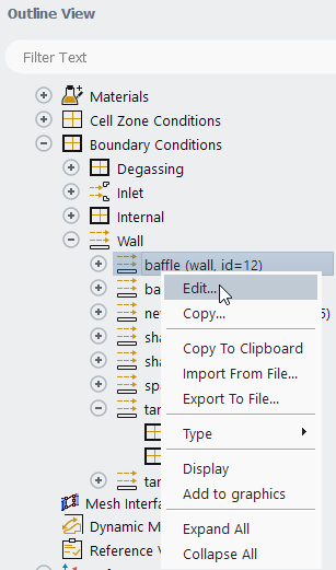
The steps you need to perform for each boundary are as follows:
Select the boundary that you want to edit from the Outline View tree, right-click the boundary and click Edit....
Set the conditions for the mixture at this boundary, if necessary. (For information about which conditions need to be set for the mixture, refer to Boundary and Cell Zone Conditions for the Mixture and the Individual Phases.)
In the boundary condition dialog box for the selected zone type (for example, the Pressure Inlet dialog box for the Eulerian model, shown in Figure 26.19: The Pressure Inlet Dialog Box for a Mixture), specify the mixture boundary conditions.
Note that only those conditions that apply to all phases, as described in Boundary and Cell Zone Conditions for the Mixture and the Individual Phases, will appear in this dialog box.
For information about inputs related to the relevant boundary conditions, refer to the appropriate sections for those boundary conditions.
If you have enabled the Wall Adhesion option in the Multiphase Model dialog box (Phase Interaction > Forces) tab, you need to specify the contact angle at the wall for each pair of phases as a constant (as shown in Figure 26.20: The Wall Dialog Box for a Mixture in a Multiphase Calculation with Wall Adhesion) or a user-defined function (see the Fluent Customization Manual for more information).
The contact angle (
 in Figure 26.21: Measuring the Contact Angle) is the angle
between the wall and the tangent to the interface at the wall, measured inside the
phase listed in the left column under Wall Adhesion in the
Momentum tab of the Wall dialog box.
For example, if you are setting the contact angle between the air and water phases
in the Wall dialog box shown in Figure 26.20: The Wall Dialog Box for a Mixture in a Multiphase Calculation with Wall
Adhesion,
in Figure 26.21: Measuring the Contact Angle) is the angle
between the wall and the tangent to the interface at the wall, measured inside the
phase listed in the left column under Wall Adhesion in the
Momentum tab of the Wall dialog box.
For example, if you are setting the contact angle between the air and water phases
in the Wall dialog box shown in Figure 26.20: The Wall Dialog Box for a Mixture in a Multiphase Calculation with Wall
Adhesion,  is measured inside the air phase. For more information, refer to
Wall Adhesion in the Theory Guide.
is measured inside the air phase. For more information, refer to
Wall Adhesion in the Theory Guide.The default value for all pairs is 90 degrees, which means that the interface is normal to the adjacent wall. Note that this is different from not including wall adhesion effects (see Surface Tension in the Fluent Theory Guide).
Define additional boundary conditions that are specific to the multiphase models.
(VOF model) If you enabled the Jump Adhesion option in the Phase Interaction > Forces tab in the Multiphase Model dialog box (Global Options group box), specify the contact angle at the porous jump for each pair of phases. When the Jump Adhesion option is enabled, it becomes visible at each of the porous jump boundaries. You can enable or disable the Jump Adhesion option in the Porous Jump dialog boxes and provide the inputs for the contact angle at the desired porous jump boundary, as shown in Figure 26.22: The Porous Jump Dialog Box Displaying Jump Adhesion.
The contact angle
 is the angle at the porous jump. To constrain the contact angle at the porous jump based on porous or non-porous fluid zones, enable the Constrained Two-Sided Adhesion option. Otherwise, if it is disabled, then the forced two-sided adhesion treatment is in effect. For more detail, see Jump Adhesion.
Click once you complete the boundary condition definition for the mixture.
Set the conditions for each phase at this boundary, if necessary. (See Boundary and Cell Zone Conditions for the Mixture and the Individual Phases for information about which conditions need to be set for the individual phases.)
Select the phase from the Phase drop-down list, located in the upper-right of each boundary condition dialog box. For example, see Figure 26.23: The Wall Dialog Box for a Phase.
Specify the boundary conditions for the phase. Note that only those conditions that apply to the individual phase, as described in Boundary and Cell Zone Conditions for the Mixture and the Individual Phases, will appear in this dialog box.
(Secondary phase only) For the pressure outlet, exhaust fan or outlet vent boundary, you can specify the volume fraction specification method as one of the following options:
Backflow Volume Fraction: You can define the backflow volume fraction as a constant, a profile (see Profiles), or a user-defined function (see the Fluent Customization Manual).
From Neighboring Cell: This option does not require the specification of the backflow volume fraction, and the volume fraction value is directly taken from the neighboring cells.
In the case of reverse flow at the pressure outlet boundary, sometimes it becomes tricky to specify the correct values for the backflow volume fraction. Incorrect specification might lead to instability, convergence issues and unphysical behavior. The backflow volume fraction specification from the neighboring interior cells can be a good choice if information at the pressure outlet boundary is not known.
Click once you complete the boundary condition definition for the phase.
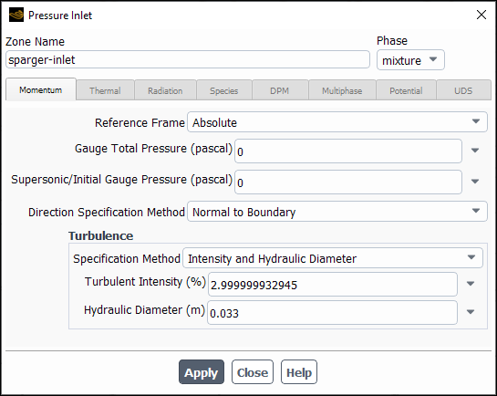
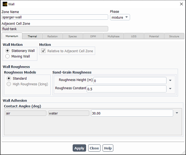
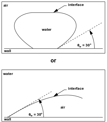
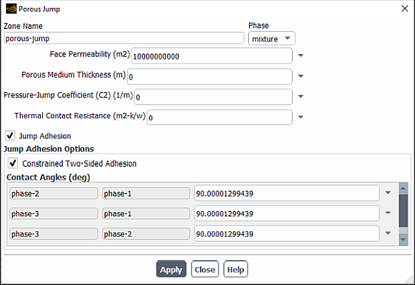
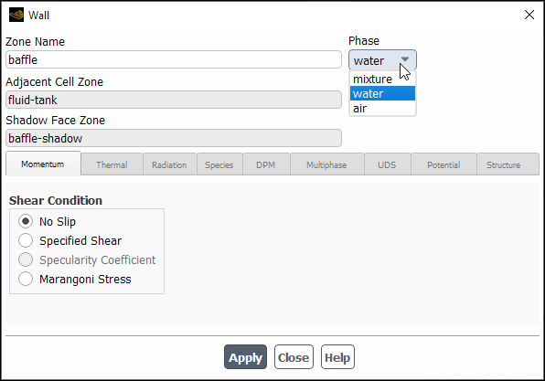
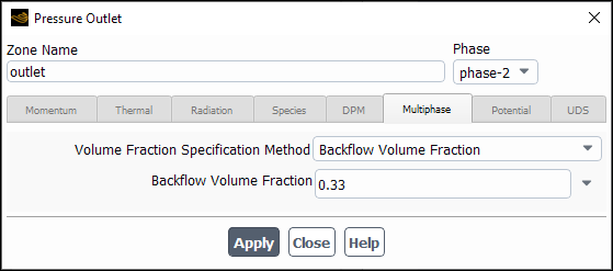
![]() Setup →
Setup → ![]() Cell Zone Conditions
Cell Zone Conditions

The steps for specifying the mixture and individual phase cell zone conditions are listed below:
Select the cell zone in the Zone list in the Cell Zone Conditions task page.
If needed, set the cell zone conditions for the mixture. (For information about which conditions need to be set for the mixture, refer to Boundary and Cell Zone Conditions for the Mixture and the Individual Phases.)
In the Phase drop-down list, select mixture.
Make sure that the selected Type is appropriate for this zone and click .
In the Fluid dialog box, set the cell zone conditions that are applicable to the mixture.
Define additional cell zone conditions that are specific to the multiphase models.
If Zonal Discretization is enabled in the Interface Modeling Options dialog box, you can specify the Compressive Scheme Slope Limiter in the Multiphase tab of the Fluid dialog box. The setting of the slope limiter can be any value between 0 and 2, inclusive. Values of 0, 1, and 2 correspond to first order upwind, second order upwind, and compressive discretization, respectively with intermediate values resulting in a blended formulation. For more details about the slope limiter, refer to The Compressive Scheme and Interface-Model-based Variants in the Fluent Theory Guide.
If required, set the conditions for each phase. (See Boundary and Cell Zone Conditions for the Mixture and the Individual Phases for information about which conditions need to be set for the individual phases.)
In the Phase drop-down list, select the phase (for example, water) and click Edit....
In the Fluid dialog box, set the cell zone conditions that are applicable to the individual phase.
For more information about inputs for cell zone conditions, see Fluid Conditions.
The boundary conditions you need to specify for the mixture and for the individual phases will depend on which multiphase model you are using.
Details for each model are provided in the following sections:
If you are using the VOF model, the conditions you need to specify for each type of boundary zone are listed below and summarized in Table 26.4: Phase-Specific and Mixture Conditions for the VOF Model.
For an inlet vent, intake fan, pressure inlet, or velocity inlet, there are no conditions to be specified for the primary phase. For each secondary phase, you will need to set the volume fraction as a constant, a profile (see Profiles), or a user-defined function (see the Fluent Customization Manual). All other conditions are specified for the mixture.
For an exhaust fan, outlet vent, or pressure outlet, there are no conditions to be specified for the primary phase. For each secondary phase, you will need to specify the volume fraction specification method as either Backflow Volume Fraction or From Neighboring Cell (see step 3. in Steps for Setting Boundary Conditions). All other conditions are specified for the mixture.
For a mass-flow inlet, you will need to set the mass flow rate, mass flux, or average mass flux for each individual phase. All other conditions are specified for the mixture.
Important: Note that if you read a VOF case that was set up in a version of Ansys Fluent prior to 6.1, you will need to redefine the conditions at the mass-flow inlets.
For an axis, fan, outflow, periodic, porous jump, radiator, solid, symmetry, or wall zone, all conditions are specified for the mixture. There are no conditions to be set for the individual phases.
For a wall zone, you can specify the contact angle for the mixture if the wall adhesion option is enabled.
For a fluid zone, mass sources are specified for the individual phases, and all other sources are specified for the mixture.
If the fluid zone is not porous, all other conditions are specified for the mixture.
If the fluid zone is porous, you will enable the Porous Zone option in the Fluid dialog box for the mixture. The porosity inputs (if relevant) are also specified for the mixture. The resistance coefficients and direction vectors, however, are specified separately for each phase. See User Inputs for Porous Media for the mixture.
If Open Channel Flow and/or Open Channel Wave BC is/are enabled in the Multiphase Model dialog box, then the Numerical Beach option becomes available under the Multiphase tab of the Fluid dialog box. To learn how to include numerical beach in your simulation, refer to Numerical Beach Treatment for Open Channels.
See Cell Zone and Boundary Conditions for details about the relevant conditions for each type of boundary. Note that the pressure far-field boundary is not available with the VOF model.
Table 26.4: Phase-Specific and Mixture Conditions for the VOF Model
| Type | Primary Phase | Secondary Phase | Mixture |
|---|---|---|---|
| inlet vent, intake fan, pressure inlet, velocity inlet | nothing | volume fraction | all others |
| exhaust fan, outlet vent, pressure outlet | nothing | volume fraction specification method | all others |
| mass-flow inlet | mass flow/flux | mass flow/flux | all others |
| axis; fan; outflow; periodic; porous jump; radiator; solid; symmetry; wall | nothing | nothing | all others |
| pressure far-field | not available | not available | not available |
| fluid | mass source; other porous inputs | mass source; other porous inputs | porous zone; porosity; all others |
If you are using the mixture model, the conditions you need to specify for each type of boundary zone are listed below and summarized in Table 26.5: Phase-Specific and Mixture Conditions for the Mixture Model.
For an exhaust fan, outlet vent, or pressure outlet, there are no conditions to be specified for the primary phase. For each secondary phase, you will need to specify the volume fraction specification method as either Backflow Volume Fraction or From Neighboring Cell (step 3 in Steps for Setting Boundary Conditions. All other conditions are specified for the mixture.
For an inlet vent, intake fan, or pressure inlet, you will specify for the mixture which direction specification method will be used at this boundary (Normal to Boundary or Direction Vector). If you select the Direction Vector specification method, you will specify the coordinate system (3D only) and flow-direction components for the individual phases. For each secondary phase, you will need to set the volume fraction (as described above). All other conditions are specified for the mixture.
For a mass-flow inlet, you will need to set the mass flow rate, mass flux, or average mass flux for each individual phase. All other conditions are specified for the mixture.
Important: Note that if you read a mixture multiphase case that was set up in a version of Ansys Fluent previous to 6.1, you will need to redefine the conditions at the mass-flow inlets.
For a velocity inlet, you will specify the velocity for the individual phases. For each secondary phase, you will need to set the volume fraction (as described above). All other conditions are specified for the mixture.
For an axis, fan, outflow, periodic, porous jump, radiator, solid, symmetry, or wall zone, all conditions are specified for the mixture. There are no conditions to be set for the individual phases. Outflow boundary conditions are not available for the cavitation model.
For a fluid zone, mass sources are specified for the individual phases, and all other sources are specified for the mixture.
If the fluid zone is not porous, all other conditions are specified for the mixture.
If the fluid zone is porous, you will enable the Porous Zone option in the Fluid dialog box for the mixture. The porosity inputs (if relevant) are also specified for the mixture. The resistance coefficients and direction vectors, however, are specified separately for each phase. See User Inputs for Porous Media for details about these inputs. All other conditions are specified for the mixture.
See Cell Zone and Boundary Conditions for details about the relevant conditions for each type of boundary. Note that the pressure far-field boundary is not available with the mixture model.
Table 26.5: Phase-Specific and Mixture Conditions for the Mixture Model
| Type | Primary Phase | Secondary Phase | Mixture |
|---|---|---|---|
| exhaust fan; outlet vent; pressure outlet | nothing | volume fraction specification method | all others |
| inlet vent; intake fan; pressure inlet | coord. system; flow direction | coord. system; flow direction; volume fraction | dir. spec. method; all others |
| mass-flow inlet | mass flow/flux | mass flow/flux | all others |
| velocity inlet | velocity | velocity; volume fraction | all others |
| axis; fan; outflow (n/a for cavitation model); periodic; porous jump; radiator; solid; symmetry; wall | nothing | nothing | all others |
| pressure far-field | not available | not available | not available |
| fluid | mass source; other porous inputs | mass source; other porous inputs | porous zone; porosity; all others |
If you are using the Eulerian model, the conditions you need to specify for each type of boundary zone are listed below and summarized in
Note that the specification of turbulence parameters will depend on which of the three multiphase turbulence models you are using, as indicated in
See Turbulence Models in the Theory Guide and Modeling Turbulence for more information about multiphase turbulence models.
For an exhaust fan, outlet vent, or pressure outlet, there are no conditions to be specified for the primary phase if you are modeling laminar flow or using the mixture turbulence model (the default multiphase turbulence model), except for backflow total temperature if heat transfer is on.
For each secondary phase, you will need to specify the volume fraction specification method as either Backflow Volume Fraction or From Neighboring Cell (step 3 in Steps for Setting Boundary Conditions. If the phase is granular, you will also need to set its backflow granular temperature. If heat transfer is on, you will also need to set the backflow total temperature.
If you are using the mixture turbulence model, you will need to specify the turbulence boundary conditions for the mixture. If you are using the dispersed turbulence model, you will need to specify them for the primary phase. If you are using the per-phase turbulence model, you will need to specify them for the primary phase and for each secondary phase.
All other conditions are specified for the mixture.
For an inlet vent, intake fan, or pressure inlet, you will specify for the mixture which direction specification method will be used at this boundary (Normal to Boundary or Direction Vector). If you select the Direction Vector specification method, you will specify the coordinate system (3D only) and flow-direction components for the individual phases. If heat transfer is on, you will also need to set the total temperature for the individual phases.
For each secondary phase, you will need to set the volume fraction (as described above). If the phase is granular, you will also need to set its granular temperature.
If you are using the mixture turbulence model, you will need to specify the turbulence boundary conditions for the mixture. If you are using the dispersed turbulence model, you will need to specify them for the primary phase. If you are using the per-phase turbulence model, you will need to specify them for the primary phase and for each secondary phase.
All other conditions are specified for the mixture.
For a mass-flow inlet, you will need to set the mass flow rate, mass flux, or average mass flux for each individual phase. You will also need to specify the temperature of each phase, since the energy equations are solved for each phase.
For mass-flow inlet boundary conditions, you can specify the slip velocity between phases. When you select a mass-flow inlet boundary for the secondary phase, two options will be available for the Slip Velocity Specification Method, as shown in Figure 26.26: Mass-Flow Inlet Boundary Condition Dialog Box :
Velocity Ratio
The value for the Velocity Ratio is the secondary phase to primary phase velocity ratio. By default, it is 1.0, which means velocities are the same (no slip). By entering a ratio that is greater than 1.0, you are indicating a larger secondary phase velocity. Otherwise, you can enter a ratio that is less than 1.0 to indicate a smaller secondary phase velocity.
Volume Fraction
If you specify the volume fraction at an inlet, Ansys Fluent will calculate the phase velocities.
Important:If a secondary phase has zero mass flux (that is, the Eulerian model is used to run a single phase case), neither Velocity Ratio nor Volume Fraction will affect the solution.
The Velocity Ratio and Volume Fraction slip velocity methods cannot be mixed for different secondary phases. That is, you should specify one or the other condition for all phases.
The volume fraction is basically the fraction of area covered by that phase.
For a velocity inlet, you will specify the velocity for the individual phases. If heat transfer is on, you will also need to set the static temperature for the individual phases.
For each secondary phase, you will need to set the volume fraction (as described above). If the phase is granular, you will also need to set its granular temperature.
If you are using the mixture turbulence model, you will need to specify the turbulence boundary conditions for the mixture. If you are using the dispersed turbulence model, you will need to specify them for the primary phase. If you are using the per-phase turbulence model, you will need to specify them for the primary phase and for each secondary phase.
All other conditions are specified for the mixture.
For an axis, outflow, degassing, periodic, solid, or symmetry zone, all conditions are specified for the mixture. There are no conditions to be set for the individual phases.
For a wall zone, shear conditions are specified for the individual phases. All other conditions are specified for the mixture, including thermal boundary conditions, if heat transfer is on.
For a fluid zone, all source terms and fixed values are specified for the individual phases, unless you are using the mixture turbulence model or the dispersed turbulence model. If you are using the mixture turbulence model, source terms and fixed values for turbulence are specified instead for the mixture. If you are using the dispersed turbulence model, they are specified only for the primary phase.
If the fluid zone is not porous, all other conditions are specified for the mixture.
If the fluid zone is porous, you will enable the Porous Zone option in the Fluid dialog box for the mixture. The porosity inputs (if relevant) are also specified for the mixture. The resistance coefficients and direction vectors, however, are specified separately for each phase. See User Inputs for Porous Media for details about these inputs. All other conditions are specified for the mixture.
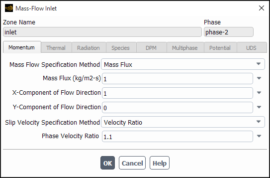
See Cell Zone and Boundary Conditions for details about the relevant conditions for each type of boundary. Note that the pressure far-field, fan, porous jump, radiator, and mass-flow inlet boundaries are not available with the Eulerian model.
Table 26.6: Phase-Specific and Mixture Conditions for the Eulerian Model (for Laminar Flow)
| Type | Primary Phase | Secondary Phase | Mixture |
|---|---|---|---|
| exhaust fan; outlet vent; pressure outlet | (tot. temperature) | volume fraction specification method; gran. temperature (tot. temperature) | all others |
| inlet vent; intake fan; pressure inlet | coord. system; flow direction (tot. temperature) | coord. system; flow direction; volume fraction; gran. temperature (tot. temperature) | dir. spec. method; all others |
| velocity inlet | velocity (tot. temperature) | velocity; volume fraction; gran. temperature (tot. temperature) | all others |
| mass-flow inlet | mass flow rate/flux (temperature) | mass flow rate/flux; velocity ratio/volume fraction; gran. temperature (temperature) | all others |
| axis; outflow; degassing; periodic; solid; symmetry | nothing | nothing | all others |
| wall | shear condition | shear condition | all others |
| pressure far-field; fan; porous jump; radiator | not available | not available | not available |
| fluid | all source terms; all fixed values; other porous inputs | all source terms; all fixed values; other porous inputs | porous zone; porosity; all |
Table 26.7: Phase-Specific and Mixture Conditions for the Eulerian Model (with the Mixture Turbulence Model)
| Type | Primary Phase | Secondary Phase | Mixture |
|---|---|---|---|
| exhaust fan; outlet vent; pressure outlet | (tot. temperature) | volume fraction specification method; gran. temperature (tot. temperature) | all others |
| inlet vent; intake fan; pressure inlet | coord. system; flow direction (tot. temperature) | coord. system; flow direction; volume fraction; gran. temperature (tot. temperature) | dir. spec. method; all others |
| velocity inlet | velocity (tot. temperature) | velocity; volume fraction; gran. temperature (tot. temperature) | all others |
| mass-flow inlet | mass flow rate/flux (temperature) | mass flow rate/flux; velocity ratio/volume fraction; gran. temperature (temperature) | all others |
| axis; outflow; degassing; periodic; solid; symmetry | nothing | nothing | all others |
| wall | shear condition | shear condition | all others |
| pressure far-field; fan; porous jump; radiator | not available | not available | not available |
| fluid | other source terms; other fixed values; other porous inputs | other source terms; other fixed values; other porous inputs | source terms for turbulence; fixed values for turbulence; porous zone; porosity; all |
Table 26.8: Phase-Specific and Mixture Conditions for the Eulerian Model (with the Dispersed Turbulence Model)
| Type | Primary Phase | Secondary Phase | Mixture |
|---|---|---|---|
| exhaust fan; outlet vent; pressure outlet | turb. parameters (tot. temperature) | volume fraction specification method; gran. temperature (tot. temperature) | all others |
| inlet vent; intake fan; pressure inlet | coord. system; flow direction; turb. parameters; (tot. temperature) | coord. system; flow direction; volume fraction; gran. temperature (tot. temperature) | dir. spec. method; all others |
| velocity inlet | velocity; turb. parameters (tot. temperature) | velocity; volume fraction; gran. temperature (tot. temperature) | all others |
| mass-flow inlet | mass flow rate/flux; turb. parameters (temperature) | mass flow rate/flux; velocity ratio/volume fraction; gran. temperature (temperature) | all others |
| axis; outflow; degassing; periodic; solid; symmetry | nothing | nothing | all others |
| wall | shear condition | shear condition | all others |
| pressure far-field; fan; porous jump; radiator | not available | not available | not available |
| fluid | momentum, mass, turb. sources; momentum, mass, turb. fixed values; other porous inputs | momentum and mass sources; momentum and mass fixed values; other porous inputs | porous zone; porosity; all |
Table 26.9: Phase-Specific and Mixture Conditions for the Eulerian Model (with the Per-Phase Turbulence Model)
| Type | Primary Phase | Secondary Phase | Mixture |
|---|---|---|---|
| exhaust fan; outlet vent; pressure outlet | turb. parameters (tot. temperature) | volume fraction specification method; turb. parameters; gran. temperature (tot. temperature) | all others |
| inlet vent; intake fan; pressure inlet | coord. system; flow direction; turb. parameters (tot. temperature) | coord. system; flow direction; volume fraction; turb. parameters; gran. temperature (tot. temperature) | dir. spec. method; all others |
| velocity inlet | velocity; turb. parameters (tot. temperature) | velocity; volume fraction; turb. parameters; gran. temperature (tot. temperature) | all others |
| mass-flow inlet | mass flow rate/flux; tub. parameters (temperature) | mass flow rate/flux; velocity ratio/volume fraction; gran. temperature (temperature) | all others |
| axis; outflow; degassing; periodic; solid; symmetry | nothing | nothing | all others |
| wall | shear condition | shear condition | all others |
| pressure far-field; fan; porous jump; radiator | not available | not available | not available |
| fluid | momentum, mass, turb. sources; momentum, mass, turb. fixed values; other porous inputs | momentum, mass, turb. sources; momentum, mass, turb. fixed values; other porous inputs | porous zone; porosity; all others |
The steps for copying cell zone and boundary conditions for a multiphase flow are slightly different from those described in Copying Cell Zone and Boundary Conditions for a single-phase flow. The modified steps are listed below:
In the Cell Zone Conditions or Boundary Conditions task page, click the button. This will open the Copy Conditions dialog box.
In the From Cell Zone or From Boundary Zone list, select the zone that has the conditions you want to copy.
In the To Cell Zones or To Boundary Zones list, select the zone or zones to which you want to copy the conditions.
In the Phase drop-down list, select the phase for which you want to copy the conditions (either mixture or one of the individual phases).
Important: Note that copying the boundary conditions for one phase does not automatically result in the boundary conditions for the other phases and the mixture being copied as well. You need to copy the conditions for each phase on each boundary of interest.
Click . Ansys Fluent will set all of the selected phase’s (or mixture’s) boundary conditions on the zones selected in the To Cell Zones or To Boundary Zones list to be the same as that phase’s conditions on the zone selected in the From Cell Zone or From Boundary Zone list. (You cannot copy a subset of the conditions, such as only the thermal conditions.)
See Copying Cell Zone and Boundary Conditions for additional information about copying boundary conditions, including limitations.
Once you have initialized the flow (as described in Initializing the Solution), you can define the initial distribution of the
phases. For a transient simulation, this distribution will serve as the initial condition
at  ; for a steady-state simulation, setting an initial distribution can
provide added stability in the early stages of the calculation.
; for a steady-state simulation, setting an initial distribution can
provide added stability in the early stages of the calculation.
You can patch an initial volume fraction for each secondary phase using the Patch Dialog Box.
![]() Solution → Initialization
Solution → Initialization
![]() Patch...
Patch...
If the region in which you want to patch the volume fraction is defined as a separate cell zone, you can simply patch the value there. Otherwise, you can create a cell “register” that contains the appropriate cells and patch the value in the register. See Patching Values in Selected Cells for details.
You have additional options for how the volume fraction is patched in a user-defined register. A standard patching procedure will initialize all the cells in the register with the specified volume fraction, without any special treatment for cells that are intersected by the fluid-fluid interface.
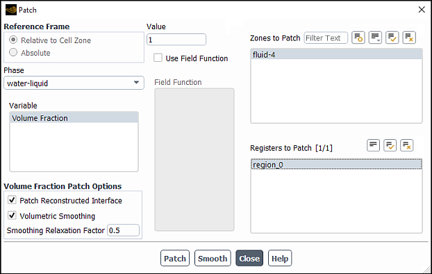
- Patch Reconstructed Interface
This option uses piecewise-linear interface reconstruction to identify the fluid-fluid interface and patches the actual volume fraction field in the cells that intersect the interface.
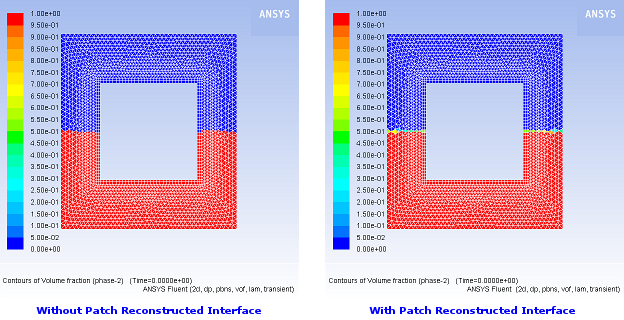
Important: The Patch Reconstructed Interface algorithm requires that the register coordinates in the dialog box be well-ordered. That is: X Min < X Max; Y Min < Y Max; Z Min < Z Max. In particular, if you use the Select Points with Mouse feature to specify the coordinates, be sure that this condition is met. If the register coordinates are not well-ordered, the register will still be created/displayed as intended; however, the volume fraction value will not be patched within the register.
The Patch Reconstructed Interface will be applied only on the last register that was defined, even if multiple registers are selected in the Patch dialog box. Therefore, it is recommended that you create and patch registers one at a time.
- Volumetric Smoothing
This option smooths the volume fraction field on-demand by taking the volumetric average over the cell neighbors. This can help provide better solution stability at startup. After enabling Volumetric Smoothing, you can click Smooth to apply the smoothing. Note that the smoothing is applied to the volume fraction field for all phases in the full domain. The Smoothing Relaxation Factor controls the degree of smoothing applied. You can specify a value between
0(no smoothing) and1(maximum smoothing). For most cases, the default value is recommended. For fine meshes you may choose to try a larger value to aid solution startup. However, excessively large values can have an undesirable effect during the solution as interface sharpening discretization schemes may deteriorate the initial field.The Smooth command can be used at any time after the solution has been initialized. It can therefore also be used after reading a data file for postprocessing. However, note that the smoothed field will overwrite the original volume fraction field in this case. Also note that you must select a secondary phase variable from the drop-down list in the Patch dialog box to expose the Volumetric Smoothing option.
By default, standard initialization uses domain-averaged values for turbulence variables, which is not ideal for a turbulent flow with multiple phases that have different properties and velocities. Ill-posed initial conditions for turbulence may result in unstable solution, especially at the start of the simulation.
For the VOF and Mixture multiphase models, you can enable the Localized Turbulence Initialization option to obtain a better initial guess for turbulence variables, which will promote better startup and run-time stability.
Once you initialize the flow, all turbulent flow variables relevant to the turbulence model will be initialized based on local velocity and local property in each cell. This type of initialization assumes the turbulent intensity of 5% and the turbulent viscosity ratio of 10. You can adjust these values using the following text commands:
solve/initialize/mp-localized-turb-init/enable
enable localized initialization of turbulent flow variables?
            [no]
yes
solve/initialize/mp-localized-turb-init/turb-init-parameters
turbulent intensity [0.05]
turbulent viscosity ratio [10]
Note that domain-averaged values displayed in the Initial Values group box in the Solution Initialization task page will be overwritten by the variable turbulence field. You can examine this field by displaying contours of Turbulence.
If executing the Patch or Smooth commands leads to a change in initial conditions, initial values of turbulent flow variables will be automatically recalculated.