


Open channel wave boundary conditions allow you to simulate the propagation of regular/irregular waves, which is useful in the marine industry for analyzing wave kinematics and wave impact loads on moving bodies and offshore structures.
Small amplitude wave theories are generally applicable to lower wave steepness and lower relative height, while finite amplitude wave theories are more appropriate for either increasing wave steepness or increasing relative height. Wave steepness is generally defined as the ratio of wave height to wave length, and relative height is defined as the ratio of wave height to the liquid depth.
Ansys Fluent provides the following options for incoming surface gravity waves through velocity inlet boundary conditions:
First order Airy wave theory, which is applied to small amplitude waves in shallow to deep liquid depth ranges, and is linear in nature.
Higher order Stokes wave theories, which are applied to finite amplitude waves in intermediate to deep liquid depth ranges, and are nonlinear in nature.
Higher order Cnoidal/Solitary wave theories, which are applied to finite amplitude waves in shallow depth ranges, and are nonlinear in nature.
Superposition of linear waves, which is used to generate various physical phenomena such as interference, betas, standing waves, and irregular waves.
Long/Short-crested wave spectrums, which are used for modeling nonlinear random waves in intermediate to deep liquid depth ranges based on a wave energy distribution function.
Short gravity wave expressions for each wave theory are based on infinite liquid height, whereas shallow or intermediate wave expressions are based on finite liquid height.
The wave height  is defined as follows:
 | (14–49) |
where  is the wave amplitude,
  is the wave amplitude at the trough, and
  is the wave amplitude at the
crest. For linear wave theory,
is the wave amplitude at the
crest. For linear wave theory,  and
for nonlinear wave theory,
and
for nonlinear wave theory,  .
.
The wave number ( ) is:
) is:
 | (14–50) |
where  is the wave length.
The vector form for the wave number  is
is
 | (14–51) |
where  is
the reference wave propagation direction,
is
the reference wave propagation direction,  is the direction opposite to gravity and
  is the direction normal to
  and
and  .
The wave numbers in the
.
The wave numbers in the  and
and  directions are defined by Equation 14–52 and Equation 14–53, respectively:
 | (14–52) |
 | (14–53) |
 is the wave heading angle, which is defined
as the angle between the wavefront and reference wave propagation
direction, in the plane of
is the wave heading angle, which is defined
as the angle between the wavefront and reference wave propagation
direction, in the plane of  and
and  .
.
The effective wave frequency  is defined as
 | (14–54) |
where  is the wave frequency and
  is the averaged velocity of the flow current.
The effects of a moving object could also be incorporated with the
flow current when the flow is specified relative to the motion of
the moving object.
is the averaged velocity of the flow current.
The effects of a moving object could also be incorporated with the
flow current when the flow is specified relative to the motion of
the moving object.
The wave speed or celerity  is defined as
 | (14–55) |
The final velocity vector for incoming waves obtained by superposing all the velocity components is represented as:
 | (14–56) |
where  ,
,  , and
, and  are the velocity components of
the surface gravity wave in the
are the velocity components of
the surface gravity wave in the  ,
,  , and
, and  directions,
respectively.
directions,
respectively.
The variable  is used in all of the wave theories and is defined
as:
is used in all of the wave theories and is defined
as:
 | (14–57) |
 and
and  are the space coordinates in the
  and
and  directions,
respectively,
directions,
respectively,  is the phase difference, and
  is the time.
The wave profile for a linear wave is given as
 | (14–58) |
where  is as define as above in Open Channel Wave Boundary Conditions.
The wave frequency  is defined as follows for shallow/intermediate
waves:
is defined as follows for shallow/intermediate
waves:
 | (14–59) |
and as follows for short gravity waves:
 | (14–60) |
where  is the liquid height,
  is the wave number, and
  is the gravity magnitude.
The velocity components for the incident wave boundary condition can be described in terms of shallow/intermediate waves and short gravity waves.
Velocity Components for Shallow/Intermediate Waves
 | (14–61) |
 | (14–62) |
Velocity Components for Short Gravity Waves
 | (14–63) |
 | (14–64) |
where  is the height from the free surface level in the
direction
is the height from the free surface level in the
direction  ,
which is opposite to that of gravity. For more information on how
to use and set up this model, refer to Modeling Open Channel Wave Boundary Conditions in the User’s
Guide.
,
which is opposite to that of gravity. For more information on how
to use and set up this model, refer to Modeling Open Channel Wave Boundary Conditions in the User’s
Guide.
Fluent formulates the Stokes wave theories based on the work by John D. Fenton[174]. These wave theories are valid for high steepness finite amplitudes waves operating in intermediate to deep liquid depth range.
The generalized expression for wave profiles for higher order Stokes theories (second to fifth order) is given as
 | (14–65) |
The generalized expression for the associated velocity potential is given as
 | (14–66) |
Where,
 | (14–67) |
 is referred to as wave steepness.
 = wave theory index (2 to 5: From 2nd order Stokes to 5th order
Stokes respectively).
= wave theory index (2 to 5: From 2nd order Stokes to 5th order
Stokes respectively).
Wave celerity,  is given as
 | (14–68) |
For 2nd order Stokes,  . (Therefore, 2nd order Stokes uses the same dispersion relation as
used by first order wave theory.) For 3rd and 4th order Stokes,
. (Therefore, 2nd order Stokes uses the same dispersion relation as
used by first order wave theory.) For 3rd and 4th order Stokes,  .
.
 = complex expressions of
  as discussed in [174].
Wave frequency,  , is defined as
 | (14–69) |
Velocity components for surface gravity waves are derived from the velocity potential function.
 | (14–70) |
 | (14–71) |
 | (14–72) |
Fluent formulates the Cnoidal/Solitary wave theories that are expressed using complex Jacobian and elliptic functions based on the work by John D. Fenton (1998) [175]. The cnoidal solution displays long flat troughs and narrow crests of real waves in shallow waters. In the limit of infinite wavelength, the cnoidal solution describes a solitary wave as a wave with a single hump, having no troughs. Due to the complexity of the cnoidal wave theories, solitary wave theories are more widely used for shallow depth regimes.
Note: For simplicity, the higher order terms, which are functions of relative height, have been omitted from the numerical details below. Refer to the work of John D. Fenton [175] for detailed numerical expressions.
The elliptic function parameter,  , is calculated by solving the
following nonlinear equation:
, is calculated by solving the
following nonlinear equation:
 | (14–73) |
Trough height from the bottom,  , is derived from the following relationship:
 | (14–74) |
Wave number,  , is defined as:
 | (14–75) |
Wave celerity,  , is defined as:
 | (14–76) |
Wave frequency,  , is defined as:
 | (14–77) |
The wave profile for a shallow wave is defined as:
 | (14–78) |
Where  is defined as:
 | (14–79) |
where  is the translational distance from reference frame
origin in the
is the translational distance from reference frame
origin in the  direction.
Velocity components for the fifth order wave theories are expressed as:
 | (14–80) |
 | (14–81) |
 | (14–82) |
where  are
the numerical coefficients mentioned in the reference [175].
are
the numerical coefficients mentioned in the reference [175].


Applying linear versus nonlinear wave theories to shallow waves is limited by the Ursell number. For nonlinear waves, the Ursell number criterion is based on waves being single-crested, without producing any secondary crests at the trough. Wave theories should be chosen in accordance with wave steepness and relative height, as waves try to acquire a nonlinear pattern with increasing wave steepness or relative height. Second and fourth order wave theories are more prone to produce secondary crests. Choosing the correct wave theory for a particular application depends on the input parameters within the wave breaking and stability limit, as described below:
Mandatory Check for Complete Wave Regime within Wave Breaking Limit
The wave height to liquid depth ratio
 (relative height) within the wave breaking limit
is defined as:
(relative height) within the wave breaking limit
is defined as:
(14–83)

(14–84)
The wave height to wave length depth ratio
 (wave steepness) within the breaking limit is defined
as:
(wave steepness) within the breaking limit is defined
as:
(14–85)

(14–86)
Check for Wave Theories within Wave Breaking and Stability Limit
For this check, the wave type is represented with the appropriate wave theory in the following manner:
Linear Wave: Airy Wave Theory
Stokes Wave: Fifth Order Stokes Wave Theory
Shallow Wave: Fifth Order Cnoidal/Solitary Wave Theory
Checks for wave theories between second to fourth order are performed between linear and fifth order Stokes wave.
Wave Regime Check
The liquid height to wave length ratio
 for short gravity waves is defined as:
(14–87)
For Stokes waves the ratio is defined as:

(14–88)
For shallow waves, the ratio is defined as:

(14–89)
Wave Steepness Check
The wave height to wave length ratio
 for linear waves is defined as:
(14–90)
For Stokes waves the ratio is defined as:

(14–91)
Note: Stokes waves are generally stable for a wave steepness below 0.1. Waves may be either stable or unstable in the range of 0.1 to 0.12. Waves are most likely to break at wave steepness values above 0.12.
For shallow waves, the ratio is defined as:

(14–92)
Relative Height Check
The wave height to liquid depth ratio
 for a linear wave is defined as:
(14–93)
For Stokes wave in shallow regime the ratio is defined as:

(14–94)
Note: Stokes waves are generally stable for a relative height below 0.4. Waves are most likely to break at a relative height above 0.4.
For shallow waves, the ratio is defined as:

(14–95)
Ursell Number Stability Criterion
The Ursell number is defined as:

(14–96)
The Ursell number stability criterion for a linear wave is defined as:

(14–97)
The criterion for Stokes wave in shallow regime is defined as:

(14–98)
Note: Stokes waves are generally stable for
 .
.Ursell numbers between 10 and 26 represent the transition to a shallow regime, therefore Stokes waves could be unstable. Stokes waves are more applicable in intermediate and deep liquid depth regimes.
The criterion for shallow waves is defined as:

(14–99)
The principle of superposition of waves can be applied to two or more waves simultaneously passing through the same medium. The resultant wave pattern is produced by the summation of wave profiles and velocity potentials of the individual waves. Depending on the nature of the superposition, the following phenomena are possible:
Interference: Superposition of waves of the same frequency and wave heights, travelling in the same direction. Constructive interference occurs in cases of waves travelling in the same phase, while destructive interference occurs in cases of waves travelling in opposite phases.
Beats/Wave Group: Superposition of waves of same wave heights travelling in the same direction with nearly equal frequencies. The beats are generated by increase/decrease in the resultant frequency of the waves over time.
For marine applications, this concept of wave superposition is known as a Wave Group. In a wave group, packets (group) of waves move with a group velocity that is slower than the phase speed of each individual wave within the packet.
Stationary/Standing Waves: Superposition of identical waves travelling in opposite directions. This superposition forms a stationary wave where each particle executes simple harmonic motion with the same frequency but different amplitudes.
Irregular Waves: Superposition of waves with different wave heights, frequencies, phase differences, and direction of propagation. Irregular sea waves are quite common in marine applications, and can be modeled by superimposing multiple waves.
Note: The superposition principle is only valid for linear and small-amplitude waves. Superposition of finite amplitude waves may be approximate or invalid because of their nonlinear behavior and dependency of the wave dispersion on wave height.
Random waves on the sea surface are generated by the action of the wind over the free surface. The higher the wind speed, the longer the wind duration, and the longer the distance over which the wind blows (fetch), the larger the resulting waves. You can simulate random wave action for open channel wave boundary conditions by specifying a wave spectrum that describes the distribution of energy over a range of wave frequencies. Fluent provides several formulations for wave spectra based on wind speed, direction, duration, and fetch.
- Fully Developed Sea State
When the wind blown over the sea imparts its maximum energy to the waves, the sea is said to be fully developed. This means that the sea state is independent of the distance over which the wind blows (fetch) and the duration of the wind. Sea elevation can be assumed as statistically stable in this case.
The sea state is often characterized by the following parameters which can be estimated from the wind speed and fetch:
- Significant Wave Height (Hs)
Mean wave height of the largest 1/3 of waves.
- Peak Wave Frequency (ωp) or Period
The frequency or period corresponding to the highest wave energy.
- Long-Crested Sea
If the irregularity of the observed waves are only in the dominant wind direction, such that there are mainly unidirectional waves with different amplitudes but parallel to each other, the sea is referred to as a long-crested irregular sea.
- Short-Crested Sea
When irregularities are apparent along the wave crests in multiple directions, the sea is referred to as short-crested.
Long-crested random wave spectrums are unidirectional and are a function of frequency only.
Ansys Fluent provides the following wave frequency spectrum formulations:
The Pierson-Moskowitz spectrum is valid for a fully developed sea and assumes that waves come in equilibrium with the wind over an unlimited fetch [3].
 | (14–100) |
| where: | |
 = Wave frequency = Wave frequency | |
 = Peak wave frequency = Peak wave frequency | |
 = Significant Wave Height = Significant Wave Height |
The JONSWAP spectrum is a fetch-limited version of the Pierson-Moskowitz spectrum in which the wave spectrum is considered to continue to develop due to nonlinear wave-wave interactions for a very long time and distance. The peak in the wave spectrum is more pronounced compared to the Pierson-Moskowitz spectrum [3].
 | (14–101) |
| where: | |
 = Pierson-Moskowitz spectrum = Pierson-Moskowitz spectrum | |
 = Wave frequency = Wave frequency | |
 = Peak wave frequency = Peak wave frequency | |
 = Peak shape parameter = Peak shape parameter | |

| |
 = Spectral width parameter = Spectral width parameter | |

|
The TMA spectrum is a modified version of the JONSWAP wave spectrum that is valid for finite water depth [3].
 | (14–102) |
 is a depth function given by:
 | (14–103) |
k is the wave number calculated from the dispersion relation

where g is the magnitude of gravity and h is the liquid depth.
Short-crested random waves are multidirectional and are a function of both frequency and direction. The short-crested wave spectrum is expressed as:
 | (14–104) |
| where: | |
 = Frequency spectrum = Frequency spectrum | |
 = Directional spreading function = Directional spreading function |
The following equation must be satisfied:

which imposes the following condition on the spreading function:

| where: | |

| |

| |
 = Principal (mean) wave heading angle = Principal (mean) wave heading angle | |
 = Angular spread
from = Angular spread
from 
|

Ansys Fluent offers two options for specifying the directional spreading
function, 


Series of individual wave components are generated for the given frequency range and angular spread. These are then superposed using linear wave theory.
For each wave component, the amplitude is calculated from:
 | (14–107) |
The final wave profile after superposing all the individual wave components is given by:
 | (14–108) |
| where: | |
 = Number of frequency components = Number of frequency components | |
 = Number of angular components = Number of angular components | |
 = Amplitude of individual wave component = Amplitude of individual wave component | |

| |
 = Wave number for
nth frequency component = Wave number for
nth frequency component | |
 = Heading angle
for the mth angular component = Heading angle
for the mth angular component | |
 = Random phase difference uniformly distributed
between 0 and 2π = Random phase difference uniformly distributed
between 0 and 2π |


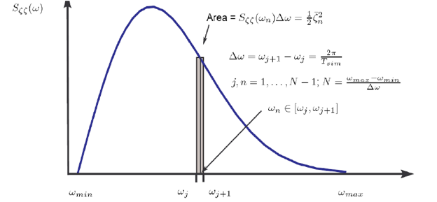
The wave spectrum is represented by a wave energy distribution
function characterized by two basic inputs: Significant Wave Height
( ) and Peak Angular Frequency (
 ). In addition, you
will enter the minimum and maximum wave frequencies (
). In addition, you
will enter the minimum and maximum wave frequencies ( and
and  ) and the number
of frequencies at which to evaluate the spectrum. You should select
the frequency range in such a way that most of the wave energy is
contained in the specified range. In general, the recommended frequency
range is:
) and the number
of frequencies at which to evaluate the spectrum. You should select
the frequency range in such a way that most of the wave energy is
contained in the specified range. In general, the recommended frequency
range is:
Minimum Angular Frequency, 
|
Maximum Angular Frequency, 
|
When choosing the spectrum and input values, it is important to analyze and consider various parameters of the resulting waves. Fluent can compute various metrics based on your inputs and assess whether the chosen spectrum and parameters are appropriate. The metrics that are computed are detailed below.
Estimation of Wave Lengths
The wave length is given by 
where  is the wave number which is calculated from the
following relationships:
is the wave number which is calculated from the
following relationships:
For intermediate depth:  , , |
For short gravity waves:  , , |
Thus,
Minimum wave length: 
|
Maximum wave length: 
|
Peak wave length: 
|
Estimation of Time Periods
The peak time period is given by 
The mean time period and the zero-upcrossing time periods are approximated as follows.
Mean time period: 
|
Zero upcrossing period: 
|
where  is the peak shape parameter.
Wave Regime Check
For the short gravity wave assumption, you should ensure that:

In general, the TMA spectrum is appropriate for intermediate depth, while the JONSWAP and Pierson-Moskowitz spectrums are valid under the short gravity wave assumption.
Relative Height Check
For the intermediate/deep treatment to be valid, the relative height should satisfy:

Sea Steepness Check
The sea steepness is computed in two ways:
based on peak time period 
based on zero-upcrossing time period 
and compared with limiting relations for each method:

Estimation of Peak Shape Parameter
The peak shape parameter,  is estimated by:

Note: For  , the JONSWAP spectrum reduces to the Pierson-Moskowitz
spectrum.
, the JONSWAP spectrum reduces to the Pierson-Moskowitz
spectrum.
|
Symbol |
Description |
|---|---|
 |
Reference wave propagation direction |

|
direction normal
to |

|
Direction opposite to gravity |
|
|
Wave Height |
|
|
Significant Wave Height |
|
|
Wave Steepness |
|
|
Wave Amplitude |
|
|
Liquid Height |
|
|
Trough Height |

| Peak Shape Parameter |
|
|
Wave Length |
|
|
Wave Heading Angle |
|
|
Wave Number |
|
|
Wave
Number in the |
|
|
Wave
Number in the |
|
|
Wave Celerity |
|
|
Wave Frequency |
|
|
Effective Wave Frequency |
|
|
Peak Wave Frequency |
|
|
Elliptical Function Parameter |
|
|
Complete Elliptical Integral of the First Kind |
|
|
Complete Elliptical Integral of the Second Kind |
|
|
Jacobian Elliptic Functions |
|
|
Spatial coordinate in the |
|
|
Spatial coordinate
in the |
|
|
Spatial coordinate in the |
|
|
Translational
distance from reference frame origin in the |
|
|
Velocity Potential |
|
|
Averaged velocity of flow current |
|
|
Velocity components for surface gravity waves in
the |


