


The procedure for computing sound using the FW-H acoustics model in Ansys Fluent consists largely of two steps. In the first step, a time-accurate flow solution is generated from which time histories of the relevant variables (for example, pressure, velocity, and density) on the selected source surfaces are obtained. In the second step, sound pressure signals at the user-specified receiver locations are computed using the source data collected during the first step.
Important: Note that you can also use the FW-H model for a steady-state simulation in the case
where your model has a single moving reference frame. Here, the thickness and loading noise
due to the motion of the noise sources is computed using the FW-H integrals (see Equation 11–5 and Equation 11–6 in the Theory
Guide), except that the term involving the time derivative of surface pressure
(contribution to  in Equation 11–6 in the Theory Guide) is set to zero.
In computing sound pressure using the FW-H integral solution, Ansys Fluent uses a so-called “forward-time projection” to account for the time delay between the emission time (the time at which the sound is emitted from the source) and the reception time (the time at which the sound arrives at the receiver location). The forward-time projection approach enables you to compute sound at the same time “on the fly” as the transient flow solution progresses, without having to save the source data.
In this section, the procedure for setting up and using the FW-H acoustics model is outlined first, followed by detailed descriptions of each of the steps involved. Remember that only the steps that are pertinent to acoustics modeling are discussed here. For information about the inputs related to other models that you are using in conjunction with the FW-H acoustics model, see the appropriate sections for those models.
The general procedure for carrying out an FW-H acoustics calculation in Ansys Fluent is as follows:
Calculate a converged flow solution. For a transient case, run the transient solution until you obtain a “statistically steady-state” solution as described below.
Enable the FW-H acoustics model and set the associated model parameters.
 Setup → Models
→ Acoustics
Setup → Models
→ Acoustics  Edit...
Specify the source surface(s) and choose the options associated with acquisition and saving of the source data. For a steady-state case, specify the rotating surface zone(s) as the source surface(s).
Specify the receiver location(s).
Continue the transient solution for a sufficiently long period of time and save the source data (transient cases only).
Solution →  Run
Calculation
Run
Calculation
Compute and save the sound pressure signals.
Solution → Run
Calculation → Acoustic Signals...
Postprocess the sound pressure signals.
Results → Plots
→ FFT Edit...
Important: Before you start the acoustics calculation for a transient case, an Ansys Fluent transient solution should have been run to a point where the transient flow field has become “statistically steady”. In practice, this means that the unsteady flow field under consideration, including all the major flow variables, has become fully developed in such a way that its statistics do not change with time. Monitoring the major flow variables at selected points in the domain is helpful for determining if this condition has been met.
As discussed earlier, URANS, LES, and hybrid RANS-LES models are all legitimate candidates for transient flow calculations. For stationary source surfaces, the frequency of the aerodynamically generated sound heard at the receivers is largely determined by the time scale or frequency of the underlying flow. Therefore, one way to determine the time-step size for the transient computation is to make it small enough to resolve the smallest characteristic time scale of the flow at hand that can be reproduced by the mesh and turbulence adopted in your model.
Once you have obtained a statistically stationary flow-field solution, you are ready to acquire the source data.
For additional information, see the following sections:
To enable the FW-H acoustics model, select Ffowcs Williams & Hawkings in the Acoustics Model dialog box (Figure 23.1: The Acoustics Model Dialog Box).
![]() Setup → Models →
Acoustics
Setup → Models →
Acoustics ![]() Edit...
Edit...
When you select Ffowcs Williams & Hawkings, the dialog box will expand to show the relevant fields for user inputs.
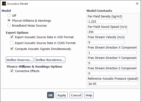
Under Model Constants in the Acoustics Model dialog box, specify the relevant acoustic parameters and constants used by the model.
- Far-Field Density
(for example,
 in Equation 11–1 in the
Theory Guide) is the
far-field fluid density.
in Equation 11–1 in the
Theory Guide) is the
far-field fluid density.- Far-Field Sound Speed
(for example,
 in Equation 11–1) is the
sound speed in the far field (=
in Equation 11–1) is the
sound speed in the far field (=  ).
).- Free Stream Velocity and Free Stream Direction
are required when the convective effects are taken into account. They become available in the interface when Convective Effects is enabled.
Important: The use of Convective Effects with the proper Free Stream Velocity and Free Stream Direction is strongly recommended for all cases dealing with external flows around bodies.
- Reference Acoustic Pressure
(for example,
 in Equation 40–15) is used to calculate
the sound pressure level in dB (see Using the FFT Utility). The default reference acoustic pressure is
in Equation 40–15) is used to calculate
the sound pressure level in dB (see Using the FFT Utility). The default reference acoustic pressure is  Pa.
Pa.- Number of Time Steps Per Revolution
is available only for steady-state cases that have a single moving reference frame. Here you will specify the number of equivalent time steps that it will take for the rotating zone to complete one revolution.
- Number of Revolutions
is available only for steady-state cases that have a single moving reference frame. Here you will specify the number of revolutions that will be simulated in the model.
- Source Correlation Length
is required when sound is to be computed using a 2D flow result. The FW-H integrals will be evaluated over this length in the depth-wise direction using the identical source data (see Figure 23.2: The Acoustics Model Dialog Box for a 3D Steady-State Case with a Single Moving Reference Frame).
The default values are appropriate for sound propagating in air at atmospheric pressure and temperature.
The FW-H acoustics model in Ansys Fluent allows you to perform simultaneous calculation of the sound pressure signals at the prescribed receivers without having to write the source data to files, which can save a significant amount of disk space on your machine. To enable this “on-the-fly” calculation of sound, enable the Compute Acoustic Signals Simultaneously option in the Acoustics Model dialog box.
Important: Because the noise computation takes a negligible percentage of memory and computational time compared to a transient flow calculation, this option can be used by itself or along with the process of source data file export and sound calculation. For the latter, computing signals “on the fly” allows you to see when the signals have become statistically steady so you can know when to stop the simulation.
When the Compute Acoustic Signals Simultaneously option is
enabled, the Ansys Fluent console window will print a message at the end of each time step
indicating that the sound pressure signals have been computed (for example,
Computing sound signals at x receiver locations..., where
x is the number of receivers you specified). Enabling this
option instructs Ansys Fluent to compute sound pressure signals at the end of each time step,
which will slightly increase the computation time.
Important: Note that this option is available only when the FW-H acoustics model has been enabled. See below for details about exporting source data without enabling the FW-H model.
Although the “on-the-fly” capability is a convenient feature, you will want to save the source data as well, because the acquisition of source data during a transient flow-field calculation is the most time-consuming part of acoustics computations, and you most likely will not want to discard it. By saving the source data, you can always reuse it to compute the sound pressure signals at new or additional receiver locations.
To save the source data to files, enable either the Export Acoustic Source Data in ASD Format or the Export Acoustic Source Data in CGNS Format option, or both. After you have made your selection, the relevant source data at all face elements of the selected source surfaces will be written into the files you specify. The source data vary depending on the solver option you have chosen and whether the source surface is a wall or not. Table 23.1: Source Data Saved in Source Data Files shows the flow variables saved as the source data.
Figure 23.2: The Acoustics Model Dialog Box for a 3D Steady-State Case with a Single Moving Reference Frame
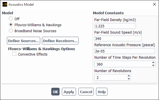
Table 23.1: Source Data Saved in Source Data Files
| Solver Option | Source Surface | Source Data |
|---|---|---|
| incompressible | walls |

|
| incompressible | permeable surfaces |

|
| compressible | walls |

|
| compressible | permeable surfaces |

|
See Specifying Source Surfaces for details on how to specify parameters for exporting source data.
You can export sound source data for use with SYSNOISE without having to enable the
Ffowcs Williams and Hawkings (FW-H) model. You still must specify source surfaces (see
Specifying Source Surfaces), as .index
and .asd files are required by SYSNOISE. In addition, you can
choose fluid zones as emission sources if you want to export quadrupole sources. To
enable the selection of fluid zones as sources, use the
define → models →
acoustics →
export-volumetric-sources?
text command and change the selection to yes.
SYSNOISE also requires centroid data for source zones that are being exported.
For fan noise calculations, once you have specified the source zones in the Acoustic Sources dialog box and you have selected Export Acoustic Source Data in ASD Format from the Acoustics Model dialog box, you can export geometry in cylindrical coordinates by using the
define → models →
acoustics →
cylindrical-export?
text command and changing the selection to yes. By default,
Ansys Fluent exports source zones for SYSNOISE in Cartesian coordinates.
You can then export the centroid data to a data file using the following text command:
define → models →
acoustics →
write-centroid-info
Since you will not be using the FW-H model to compute signals, you will not need to specify any acoustic model parameters or receiver locations. Also, you will not be able to enable the Compute Acoustic Signals Simultaneously option in the Acoustics Model dialog box, and Acoustic Signals... will not be available in the Run Calculation task page and in the menu for the Run Calculation Outline View item.
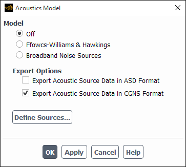
The sound source data for non-permeable surfaces can be exported in the CGNS file
format (for Simcenter 3D Acoustics) without having to enable the Ffowcs Williams and
Hawkings (FW-H) model. Enable the Export Acoustic Source Data in CGNS
Format option in the Acoustics Model dialog box (Figure 23.3: The Acoustics Model Dialog Box for Exporting in CGNS Format). Specify the source surfaces in the
Acoustics Sources dialog box (see Specifying Source Surfaces) where, by default, the Number of
Time Steps per File is set to 1.
Note: The following limitation currently exists for exporting acoustic source data:
Source data cannot be simultaneously exported for multiple differently rotating walls. All walls must be either non-rotating, or rotate with the same rate around the same axis. It is a responsibility of a user to select a consistent set of wall zones. Selecting differently rotating zones may cause incorrect acoustics result.
Simcenter 3D Acoustics requires a mesh data file (named
<prefix>_mesh.cgns) and a solution data file (named
<prefix>_<timestep>.cgns). The string
<prefix> is a generic name, which you will specify in
the File Name in the Acoustics Sources dialog
box. There is one single solution data file (.cgns) per time
level exported, which contains the static pressure at the wall-face centroid location.
The .cgns files will be stored in a directory, which you
specify (named <directory_name>/<prefix>) in the
File Name.
In addition, you can export quadrupole sources data by choosing fluid zones as emission sources. To enable the selection of fluid zones as sources, use the text command:
define → models →
acoustics →
export-volumetric-sources-cgns?
When asked if you would like to Export volumetric sources?
enter yes. Note that Simcenter 3D Acoustics requires volumetric
mesh data file (<prefix>_Q_mesh.cgns) and quadrupole
solution data files (<prefix>_Q_<timestep>.cgns).
The .cgns file will be stored in a similar way to that of
dipole data export, in the directory you specified in the File Name
text entry box.
In the Acoustics Model dialog box, click the button to open the Acoustic Sources dialog box (Figure 23.4: The Acoustics Model Dialog Box). Here you will specify the source surface(s) to be used in the acoustics calculation and the inputs associated with saving source data to files.
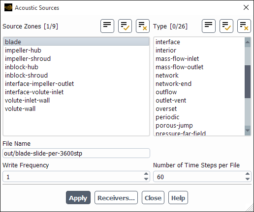
Under Source Zones, you can select multiple emission (source) surfaces and the surface Type that you can select is not limited to a wall. You can also choose interior surfaces and sliding interfaces (both stationary and rotating) as source surfaces.
Important: The ability to choose multiple source surfaces is useful for investigating the contributions from individual source surfaces. The results based on the use of multiple source surfaces are valid as long as there are negligible acoustic interactions among the surfaces. Therefore, some caution should be taken when selecting multiple source surfaces.
In cases where multiple source surfaces are selected, no source surface may enclose any of the other source surfaces. Otherwise, the sound pressure calculated based on the source surfaces will not be accurate, as the contribution from the enclosed (inner) source surfaces is over predicted, since the FW-H model is unable to account for the shading of the sound from the inner source surfaces by the enclosure surface.
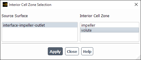
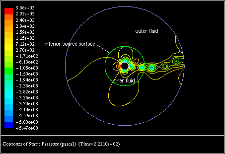
If you specify any interior surfaces as source surfaces, the interior surface must be generated in advance, in such a way that the two cell zones adjacent to the surface have different cell zone IDs. Furthermore, you must correctly specify which of the two zones is occupied by the quadrupole sources (interior cell zone). This will allow Ansys Fluent to determine the direction in which the sound will propagate. When you first attempt to select a legitimate interior surface (that is, an interior surface having two different cell zones on both sides) as a source surface, the Interior Cell Zone Selection Dialog Box (Figure 23.5: The Interior Cell Zone Selection Dialog Box) will appear. You must then select the interior cell zones from the two zones listed under the Interior Cell Zone. Figure 23.6: An Interior Source Surface shows an example of an interior source surface.
Like general interior surfaces, if the source surfaces selected are sliding interfaces, a dialog box similar to Figure 23.5: The Interior Cell Zone Selection Dialog Box will appear that will show the two adjacent cell zones and you will be asked to specify the zone that has the sound sources.
Important: When a permeable surface (either interior or sliding interface) is chosen as the source surface, other wall surfaces inside the volume enclosed by the permeable surface that generate sound should not be chosen for the acoustics calculation. For example, when running an “on-the-fly” calculation, if both these surfaces are selected, the sound pressure will be counted twice.
To save the source data, you have to specify the File Name, Write Frequency (in number of time steps), and Number of Time Steps per File in the Acoustic Sources dialog box.
The File Name is used to give the names of the source data files
(for example, acoustic_examplexxxx.asd, where
xxxx is the global time-step index of the transient solution)
and an index file (for example, acoustic_example.index) that will
store the information associated with the source data. The Write
Frequency allows you to control how often the source data will be written.
This will enable you to save disk space if the time-step size used in the transient flow
simulation is smaller than necessary to resolve the sound frequency you are attempting to
predict. In most situations, however, you will want to save the source data at every time
step and use the default value of 1.
Since acoustics calculations usually generate thousands of time steps of source data, you may want to split the data into several files. Specifying the Number of Time Steps per File allows you to write the source data into separate files for different simulation intervals, the duration of which (in terms of the number of transient flow time steps) is specified by you. For example, if you specify 100 for this parameter, each file will contain source data for an interval length of 100 time steps regardless of the write frequency.
You will find this feature useful if you want to use a selected number of source data files to compute the sound pressure rather than using all the data. For example, you may want to exclude an initial portion of the source data from your acoustics calculation because you may realize later that the flow field has not fully attained a statistically steady state.
After you click , Ansys Fluent will create the index file (for
example, acoustics_example.index), which contains information
about the source data.
Important: If you choose to save source data, keep in mind that the source data can use up a considerable amount of disk space, especially if the mesh being used has a large number of face elements on the source surfaces you selected. Ansys Fluent will print out the disk space requirement per time step at the time of source surface selection if the Export Acoustic Source Data in ASD Format option is enabled in the Acoustics Model dialog box.
At this point, if you have chosen to perform your acoustics calculation in two steps, (that is, saving the source data first, and computing the sound at a later time), you can go ahead and instruct Ansys Fluent to perform a suitable number of time steps, and the source data will be saved to the disk. If you chose to perform an “on-the-fly” acoustic calculation, then you must specify receiver locations (see Specifying Acoustic Receivers) before you run the unsteady Ansys Fluent solution any further.
In the Acoustics Model dialog box, click the button to open the Acoustic Receivers dialog box (Figure 23.7: The Acoustic Receivers Dialog Box).
Important: Note that you can also open the Acoustic Receivers dialog box by clicking the button in the Acoustic Sources or the Acoustic Signals dialog box.
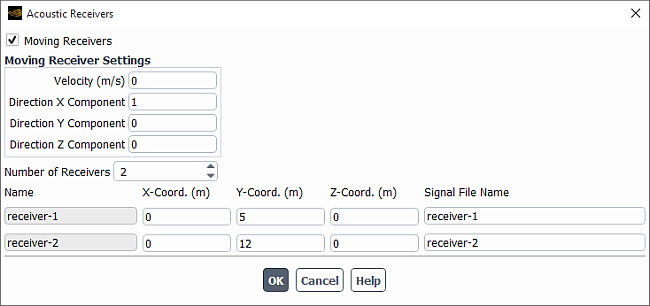
If required, you can enable Moving Receivers to specify the receiver motion. In this case, the defined Velocity magnitude and Direction apply to all receivers. The receiver locations, defined below, are then interpreted as the starting locations at the time that sound emission originates. The origination of sound emission is determined as follows:
For “on the Fly” use of the FW-H model (see Computing Sound “on the Fly”) the sound emission time is counted from the physical time of activation of the Compute Acoustic Signals Simultaneously option (see Figure 23.1: The Acoustics Model Dialog Box).
When the FW-H model reads the previously written acoustic source data (see Reading Unsteady Acoustic Source Data), the sound emission time starts from the physical time associated with the first selected source data file.
Important: When using moving receivers, note that if you start from a different source data file, this results in different receiver locations due to the different emission time origin associated with the different source data file.
Increase the Number of Receivers to the total number of receivers for which you want to compute sound, and enter the coordinates for each receiver in the X-Coord., Y-Coord., and Z-Coord. fields. Note that because Ansys Fluent’s acoustics model is ideally suited for far-field noise prediction, the receiver locations you define should be at a reasonable distance from the sources of sound (that is, the selected source surfaces). The receiver locations can also fall outside of the computational domain.
For each receiver, you can specify a file name root in the Signal File
Name field. The signal file name extension for the FW-H model is fixed to
.ard. These files will be used to store the sound pressure
signals at the corresponding receivers. By default, the files will be named
receiver-1.ard, receiver-2.ard, and so
on.
Once the receiver locations have been defined, the setup for your acoustic calculation is complete.
When using an implicit-in-time solution algorithm (dual-time stepping), and depending on the physical time step size and the most important time scales in the flow, you can write the acoustic source data at every time step. You can also coarsen it in time by a given frequency factor. The highest possible frequency the acoustic analysis can generate is based on the time step size of the collected acoustic source data.
When using the Density-Based explicit solver, with the Explicit Transient Formulation selected in the Solution Methods task page, the physical time step size must be computed by the solver, based on the CFL condition (Courant number). Due to the possibly large fluctuations of the physical time step size, an adapting time-stepping procedure can be used when the FW-H acoustics model is enabled. This allows you to use a user-specified time interval for sampling the acoustic data. In turn, the solver adapts its time step size, when necessary, without violating the CFL conditions to make sure that data is available at the desired time interval (hence, avoiding data interpolations).
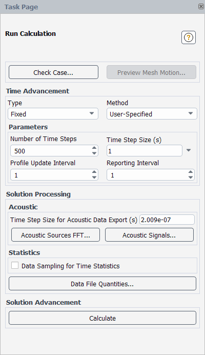
In the Run Calculation task page (Figure 23.8: The Run Calculation Task Page), enter the Time Step Size for Acoustic Data Export to specify the time interval for acoustic data sampling. The value of this constant time step size determines the highest frequency that the acoustic analysis reproduces.
You can refer to Performing Time-Dependent Calculations for more information about the Run Calculation task page.
![]() Solution →
Solution → ![]() Run
Calculation
Run
Calculation
You can now proceed to instruct Ansys Fluent to perform a transient calculation for a suitable number of time steps. When the calculation is finished, you will have either the source data saved on files (if you chose to save it to a file or files), or the sound pressure signals (if you chose to perform an acoustic calculation “on the fly”), or both (if you chose to save the source data to files and if you chose to perform the acoustic calculation “on the fly”).
If you chose to save the source data to files, the Ansys Fluent console will print a message
at the end of each time step indicating that source data have been written (or appended to)
a file (for example, acoustic_example240.asd).
At this point, you will have either the source data saved to files or the sound pressure signals computed, or both. You can process these data to compute and plot various acoustic quantities using Ansys Fluent’s FFT capabilities (Fast Fourier Transform (FFT) Postprocessing). Additionally, you can perform Ansys Sound analysis on computed pressure signals. Refer to Performing an Ansys Sound Analysis for additional information.
If you chose to perform the acoustic calculation “on the fly”, you must
write the sound pressure data to files. To do so, select Write Acoustic
Signals under Options in the Acoustic
Signals dialog box (Figure 23.9: The Acoustic Signals Dialog Box) and
then click . The computed acoustic pressure will be saved from
internal buffer memory into a separate file for each receiver you defined in the
Acoustic Receivers dialog box (for example,
receiver-1.ard).
![]() Solution →
Solution → ![]() Run
Calculation → Acoustic Signals...
Run
Calculation → Acoustic Signals...
Computing the sound pressure signals using the source data saved to files is done in the Acoustic Signals dialog box (Figure 23.9: The Acoustic Signals Dialog Box)
![]() Solution →
Solution → ![]() Run
Calculation → Acoustic Signals...
Run
Calculation → Acoustic Signals...
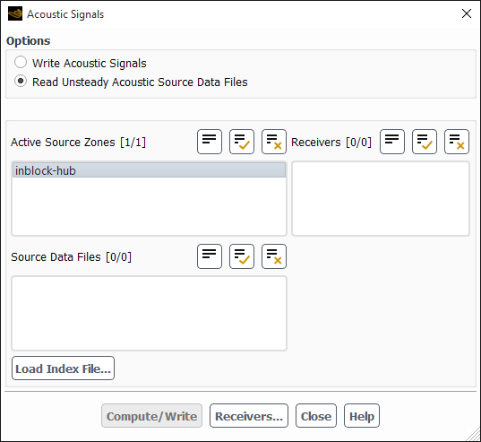
To compute the sound data, use the following procedure:
In the Acoustic Signals dialog box, select Read Unsteady Acoustic Source Data Files under Options.
Click and select the index file for your computation in the Select File dialog box. The file will have the name you entered in the File Name field in the Acoustic Sources dialog box, followed by the
.indexsuffix (for example,acoustic_example.index).In the Source Data Files list, select the source data files that you want to use to compute sound. Source data files will all contain the specified root file name followed by the suffix
.asd.Important: You can use any number of source data files. However, note that you should select only consecutive files.
In the Active Source Zones list, select the source zones you want to include to compute sound. See Specifying Source Surfaces for details about proper source surface selection.
In the Receivers list, select the receivers for which you want to compute and save sound.
Optionally, you can click the button to open the Acoustic Receivers dialog box and define additional receivers.
Click the button to compute and save the sound pressure data. One file will be saved for each receiver you previously specified in the Acoustic Receivers dialog box (for example,
receiver-1.ard).
Important: If you enabled both the Export Acoustic Source Data in ASD
Format and Compute Acoustic Signals Simultaneously
options in the Acoustics Model dialog box, you must first select
the Write Acoustic Signals option in the Acoustic
Signals dialog box after the flow simulation has been completed. If you
select the Read Unsteady Acoustic Source Data Files before writing
out the “on-the-fly” data in such a case, the data will be flushed out of
the internal buffer memory. To avoid such a loss of data, you should save the Ansys Fluent
case and data files whenever you begin to do an acoustic computation in the
Acoustic Signals dialog box. The sound pressure data calculated
“on the fly” will then be saved into the .dat
file. Finally, after the “on-the-fly” data is saved, make sure to change
the file names of the receivers before doing a sound pressure calculation with the
Read Unsteady Acoustic Source Data Files option enabled, to avoid
overwriting the “on-the-fly” signal files.
Important: Note that you can compute and write sound pressure signals only when the FW-H acoustics model has been enabled. See Exporting Source Data Without Enabling the FW-H Model: Using the Ansys Fluent ASD Format for details about exporting source data (for example, for SYSNOISE) without enabling the FW-H model.
Before the computed sound pressure data at each receiver is saved, it is by default automatically pruned. Pruning of the receiver data means clipping the tails of the signal where incomplete source information is available.
The acoustic source data is tabulated from time  to
to  . Without auto-pruning, the receiver register begins receiving the
earliest sound pressure signal at
. Without auto-pruning, the receiver register begins receiving the
earliest sound pressure signal at
 | (23–1) |
where  is the shortest distance between the source surfaces and the receiver.
However, the receiver will not receive the sound pressure signal from the farthest point
on the source surfaces (
is the shortest distance between the source surfaces and the receiver.
However, the receiver will not receive the sound pressure signal from the farthest point
on the source surfaces ( ) until the receiver time becomes
 | (23–2) |
From time  to
to  , the sound accumulated on the receiver register does not include the
contribution from the entire source surface area, and therefore the sound pressure data
received during that time is not complete. The same thing occurs during the period
from
, the sound accumulated on the receiver register does not include the
contribution from the entire source surface area, and therefore the sound pressure data
received during that time is not complete. The same thing occurs during the period
from
 | (23–3) |
to
 | (23–4) |
Therefore, pruning means clipping the signal on the incomplete ends, from
 to
to  and
and  to
to  . Auto-pruning can be disabled using the
define → models →
acoustics → auto-prune
text command. Although auto-pruning can be disabled, it is expected that you will use
only the complete sound pressure data.
The RMS value of the static pressure time derivative ( ) is available for postprocessing only on wall surfaces, which are at the
same time sources of sound, when the FW-H acoustics model is used.
) is available for postprocessing only on wall surfaces, which are at the
same time sources of sound, when the FW-H acoustics model is used.
You can select Surface dpdt RMS in the Acoustics... category only when you specify at least one wall surface, which is also marked as an acoustic source, in the relevant postprocessing dialog boxes.
Once the sound pressure signals are computed and saved in files, the sound data is
ready to be analyzed using Ansys Fluent’s FFT tools. In the Fourier
Transform dialog box (Figure 40.124: The Fourier Transform Dialog Box), click
and select the appropriate
.ard file. If the receiver data is still in Ansys Fluent’s
memory, then it can directly be processed using the Process Receiver
option. See Fast Fourier Transform (FFT) Postprocessing for more information on
Ansys Fluent’s FFT capabilities.
![]() Results → Plots
→ FFT
Results → Plots
→ FFT ![]() Edit...
Edit...
During a transient flow simulation, the time histories of the instant surface pressure values can be written into the binary acoustic source data (ASD) files. This operation is performed for all mesh cell faces of those surface zones that are selected as acoustic sources. The primary purpose of the ASD files is to supply input data for the Ffowcs Williams and Hawkings acoustic solver (see Reading Unsteady Acoustic Source Data). Additionally, these files can be used to compute and visualize the spectral properties of the stored flow pressure signals. The supported spectral properties for the individual Fourier modes are the complex amplitudes. For the frequency bands, the surface pressure level (SPL) values, in decibels, and the dimensional power spectral density (PSD) values of the pressure time derivative are provided. Both the constant width and the proportional width bands (octaves and 1/3 octaves) can be specified.
Note: Despite the use of the common acronym “SPL”, the calculated values characterize the transient flow pressure on a surface, and not the acoustic pressure; that is, in this context, the acronym refers to the “Surface Pressure Level” (as mentioned previously) and not the “Sound Pressure Level”.
In addition to the visualization capabilities, you can also use the computed spectral data to export surface fields of the complex amplitudes of flow pressure as CGNS files. The primary purpose of such files is to allow you to use the surface spectrum fields as distributed excitation forces when performing a harmonic response analysis with Ansys Mechanical. The ability to import CGNS files is available in Ansys Mechanical to match this export feature in Fluent; for details, see FLUREAD in the separate Mechanical APDL Command Reference. Using the acoustic wave equation solver of Ansys Mechanical, it is possible to perform frequency domain simulations for applications such as the vehicle cabin noise caused by external turbulent flow.
The button is available in the Run Calculation task page under the following conditions:
The simulation is set up as a three-dimensional transient case.
The Export Acoustic Source Data in ASD Format option is enabled in the Acoustics Model dialog box.
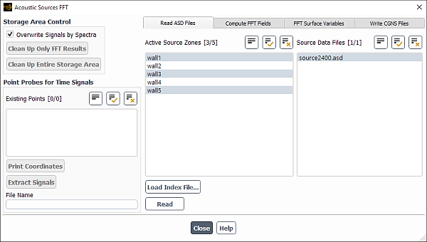
Clicking the button opens the Acoustic Sources FFT dialog box, which has four tabs (each of which is shown in the figures that follow):
Read ASD Files
Compute FFT Fields
FFT Surface Variables
Write CGNS Files
The first two tabs are obligatory, because the actions performed there prepare the Fourier spectra for the actions that follow, including creation of the surface variables to visualize (performed in the third tab) and/or CGNS export (performed in the fourth tab).
Postprocessing begins in the Read ASD Files tab. The Active Source Zones selection list shows all of the face zones for which transient export to ASD files has been performed (see Figure 23.10: The Read ASD Files Tab of the Acoustic Source FFT Dialog Box). The Source Data Files selection list shows all of the available ASD files. Note that you can update this information by clicking the button and specifying the name of the index file to be read; the index file was created during the ASD files export, and is an ASCII file containing a list of the source zones and a list of the ASD file names. Select in the selection lists the desired face zones as well as the desired ASD files from which you want to read, and click the button. The console displays information about the data, such as the following example:
Overall 10000 timesteps have been read
from 3.0001 s to 4 s
Time step is 0.0001 s
Having read the pressure histories, open the Compute FFT Fields tab (Figure 23.11: The Compute FFT Fields Tab of the Acoustic Source FFT Dialog Box). The values shown in the Spectral Resolution group box provide information about the statistical properties, which depend on the sampling rate (that is, the simulation time step size) and the signal length (that is, the simulation time). These values will change if you enable the Clip Time to Range option in the Sampling Data group box, reduce the time range for the signals by changing the Min and/or Max fields, and click the button. The Window Function selection list allows you to specify a window function using the same choices that are available for plotting the single signal FFT in the Plot/Modify Input Signal dialog box. The default settings use the full signals and the Hanning window function. The FFT calculation begins when you click the button.
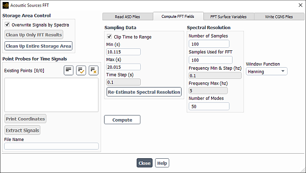
The fields of the pressure histories and the computed fields of the Fourier spectra are stored in a large memory array, referred to here as the “storage area”. This memory is allocated by Fluent dynamically when you read the pressure signals from the ASD files. If you read data for all face zones available in the ASD files, and if they are the wall zones, then the size of the allocated storage area is equal to the total size of the ASD files being read. Since the same or a slightly smaller amount of data is produced by the FFT algorithm, the same storage area can be re-used to store the Fourier spectra without allocating additional memory. Alternatively, the pressure histories can be left intact in memory, and for their spectra the storage area is correspondingly increased.
These two modes of memory allocation are controlled by the Overwrite Signals by Spectra option in the Storage Area Control group box. When the Overwrite Signals by Spectra option is enabled, the Fourier spectra displace in memory the original time signals, which are not kept after the FFT has been computed. Therefore, if you want to re-compute the FFT using the Clip Time to Range tool or a different Window Function (which are both in the Compute FFT Fields tab), you have to first de-allocate the storage area by clicking the button, and then re-read the pressure histories from the ASD files. When the Overwrite Signals by Spectra option is disabled, you can re-compute the FFT without re-reading the pressure histories, as many times as you want. To do this, click the button, and proceed with computing spectra from the available pressure histories. De-allocation of the storage area (which can be very large) is recommended when you are done using the Acoustic Sources FFT dialog box and plan to either proceed to other postprocessing work or continue your transient simulation without re-starting Fluent.
When the pressure histories are read and kept in the storage area, you can create point probes within the surface zones that have been read and extract the single pressure time signals at these probes. The extracted signals and their spectra may help to analyze the transient flow properties. For example, by creating an XY plot of a signal, you can figure out the need for clipping of the sampling time; by creating an XY plot of its spectrum, you can detect the presence of the tonal noise components.
To create a point probe, open the Point Surface Dialog Box by clicking
Create and selecting Point... in the
Domain ribbon tab (Surface group box), and
create a point surface by any available method (for example, by specifying the
coordinates). The point probe will be created at the face center that is nearest to the
point surface on the read surface zones. The created point probes are then listed under
the point surface names in the Existing Points selection list, which
is located in the Point Probes for Time Signals group box. You can
print the coordinates of the point probes to the Fluent console by selecting the desired
probes and clicking the button. Clicking the
button outputs the pressure histories for the
selected probes in the ASCII files; these files can then be analyzed using the Fourier Transform Dialog Box (available from the Plots Task Page) by selecting Process File Data
and then reading the exported ASCII file using the button. The exported files names are by default the point probe
names with the extension .dat. The File Name
field allows you to specify a prefix for these file names.
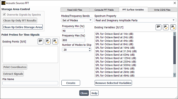
The FFT Surface Variables tab is shown in Figure 23.12: The FFT Surface Variables Tab of the Acoustic Source FFT Dialog Box for the Octave Bands and Figure 23.14: The FFT Surface Variables Tab of the Acoustic Source FFT Dialog Box for a Set of Individual Modes. This tab allows you to new Fluent variables using the computed spectrum fields, which reside in the storage area and correspondingly increase its size. These variables will be defined only on those wall face zones for which the Fourier transformation has been computed; on the other face zones, they will show zero values. Created variables can be used for any kind of further postprocessing in Fluent, which typically includes contour plotting (see the variables marked with the restriction asfft in Table 42.21: Acoustics Category ) or exporting to CFD-Post.
Figure 23.12: The FFT Surface Variables Tab of the Acoustic Source FFT Dialog Box for the Octave Bands
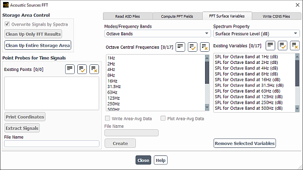
Variables may characterize either the individual Fourier modes (if you select Set of Modes from the Modes/Frequency Bands drop-down list), or frequency bands that each represent a range of frequencies (if you select the other choices in the Modes/Frequency Bands drop-down list). The three types of frequency bands that are available include:
Octave Bands
These are proportional bands corresponding to the standard technical octaves.
1/3 Octave Bands
These are proportional bands corresponding to the standard technical thirds.
Constant Width Bands
These are user-defined equidistant bands.
The Spectrum Property drop-down list displays the type of variables created according to the selected choice in the Modes/Frequency Bands drop-down list. For a set of modes, the created variables are the real and the imaginary parts of the complex Fourier amplitudes, with a pair of variables per specified mode. For the frequency bands, the two types of variables can be created:
The surface pressure level (SPL) fields, in decibels. The transformation to the decibel units is done by default using the standard acoustic reference pressure value of 2 x 10⁻⁵ Pa; you can change this value before creating the variables by opening the Acoustic Models dialog box, selecting the Ffowcs Williams & Hawkings model, and revising the Reference Acoustic Pressure.
The fields of the dimensional power spectral density (PSD) of the pressure time derivative, in units of pressure squared over time squared.
For any type of frequency band (octave, 1/3, or constant width), the area-averaged band-specific pressure fluctuations are calculated and printed out to the Fluent console in decibels when you click Create. Conversion to decibels is done after the area-averaging of the band-filtered RMS pressure fluctuation fields. Similarly, the area-averaged band-specific values of PSD of the pressure time derivative are calculated and printed out, if this variable type is selected. The area-averaged data are printed only for those frequency bands that are covered by the resulting pressure spectrum. If you enable the Write Area-Avg Data option and specify a file name in the corresponding field, then the area-averaged data will be written to an ASCII file in the XY plot file format (see XY Plot File Format). It is recommended that you use the file name extension .xy to more easily recognize this file when using the XY plotting tool.
If you enable the Plot Area-Avg Data option, then the data will be plotted in the form of a bar chart in the graphics window when you click Create, as shown in Figure 23.13: Bar Chart of Surface Pressure Level for Octave Bands.
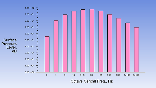
Figure 23.14: The FFT Surface Variables Tab of the Acoustic Source FFT Dialog Box for a Set of Individual Modes
The allowed number of variables makes it possible for you to simultaneously keep SPL and PSD of dp/dt for all octave and 1/3 octave bands, as well as SPL and PSD of dp/dt for up to 20 constant width bands and the real and imaginary amplitudes for up to 20 individual frequencies. The SPL and PSD of dp/dt variables for the octaves and the 1/3 octaves include the band central frequency in their names (for example, SPL for Octave Band at 250Hz (dB) or PSD of dp/dt for 1/3-Octave Band at 1.25kHz). As for the user-defined frequencies and constant width bands, their variables are simply numbered from 0 to 19. In order to provide you with the information about the meaning of each such variable, Fluent prints a table in the console when you click . The following is an example of the table corresponding to the settings in the previous figure:
Creating variables for 20 modes from 40.5983 Hz to 466.88 Hz every 22.4359 Hz.
f( 0) = 40.5983 Hz     f( 1) = 63.0342 Hz
f( 2) = 85.4701 Hz     f( 3) = 107.906 Hz
f( 4) = 130.342 Hz     f( 5) = 152.778 Hz
f( 6) = 175.214 Hz     f( 7) = 197.65 Hz
f( 8) = 220.085 Hz     f( 9) = 242.521 Hz
f(10) = 264.957 Hz     f(11) = 287.393 Hz
f(12) = 309.829 Hz     f(13) = 332.265 Hz
f(14) = 354.701 Hz     f(15) = 377.137 Hz
f(16) = 399.573 Hz     f(17) = 422.009 Hz
f(18) = 444.444 Hz     f(19) = 466.88 Hz

Variables for frequencies above 466.88 Hz are not created,
because the limit of 20 modes has been reached.
You can analyze more than 20 individual modes or constant width bands, if you process them by portions of 20 items and delete the processed variables by selecting them in the Existing Variables list and clicking the button.
Clicking either the Clean Up Entire Storage Area or the button on the left side of the dialog box not only de-allocates the spectrum storage array, but also removes all created variables.
The Write CGNS Files tab is shown in Figure 23.15: The Write CGNS Files Tab of the Acoustic Source FFT Dialog Box. This tab allows you to specify the zones you want to export to CGNS, by selecting them in the Processed Source Zones list. You can reduce the exported spectrum data by enabling the Reduce Frequency Series option and specifying the frequency range (Min and Max frequencies), as well as the frequency step (the Number of Frequencies to Skip integer field). The latter must be used with care and only if really needed, because the Fourier amplitudes in the broadband noise spectrum depend on the frequency resolution. By skipping frequencies from the exported spectrum (for example, exporting every other Fourier mode), you will artificially coarsen the frequency resolution. However, the exported amplitudes will not be automatically re-scaled for the increased frequency step, but will retain their originally computed values.
Pressure spectra, which result from the scale-resolving flow simulations, may contain thousands of frequencies. Together with dense surface meshes, this can result in a very large amount of data to export. The total size of the disk space required to store fields of the complete spectra is approximately equal to the total size of the ASD files containing the wall pressure histories. Therefore, the wall pressure spectra are written to a series of CGNS files according to the Number of Frequencies per File field. It is recommended that you select an appropriate value for this parameter, to avoid extremely large output files or a large number of very small files. The total number of frequencies in the spectrum can be seen in the Number of Modes field of the Compute FFT Fields tab (see Figure 23.11: The Compute FFT Fields Tab of the Acoustic Source FFT Dialog Box).
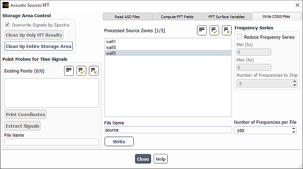
Finally, you can specify a name for the exported CGNS files in the File
Name field. For example, if you enter
wall_pressure_spectrum and then click the
button, Fluent will create the following set of files in
your working folder:
wall_pressure_spectrum.cgns
wall_pressure_spectrum_1.cgns
wall_pressure_spectrum_2.cgns
...
wall_pressure_spectrum.flst
If you leave the File Name field empty, the files will be named cgns, 1.cgns, 2.cgns, ..., flst. The first CGNS file (without a number in its name) contains the mesh data, as well as links to all of the other CGNS files, which in turn contain the spectrum fields with the specified number of modes per file. The CGNS links work like the file links in the UNIX file system: in order to import spectra to the Ansys Mechanical software, you only have to specify the name of the first file, and all other files will be imported automatically if they reside in the same folder. The file with the extension flst is an ASCII file, which contains the list of the exported frequencies.
Important: Note the following:
You should not specify a relative path as a part of the File Name input. If you do that, all files will be exported in the desired folder according to the specified path. However, the CGNS links, which are written in the first CGNS file, will also include the specified path. Therefore, the linked CGNS files will become readable only after the correspondent file relocation—for example, moving the first CGNS file in your Fluent working folder.
The public domain CGNS library, which is used to process CGNS files in Fluent and Ansys Mechanical, has a performance issue when run on Windows. Namely, for CGNS files that have many links (as is the case in this application), the input / output operations may be very slow if the CGNS files are located on a network disk. Therefore, for Windows it is strongly recommended that you select either a built-in local disk or a USB disk directly connected to your computer as the location of the CGNS files. This warning concerns both the export of CGNS files from Fluent and their import in Ansys Mechanical.