


This section discusses how to use the composition PDF transport model for modeling finite-rate chemistry in turbulent flames in Ansys Fluent. Ansys Fluent has two different discretizations of the composition PDF transport equation, namely Lagrangian and Eulerian. The Lagrangian method is more accurate than the Eulerian method, but requires significantly longer run time to converge. For information about the theory behind the composition PDF transport model, see Composition PDF Transport in the Theory Guide.
Information about using this model is presented in the following sections:
- 19.2.1. Limitation
- 19.2.2. Steps for Using the Composition PDF Transport Model
- 19.2.3. Enabling the Lagrangian Composition PDF Transport Model
- 19.2.4. Enabling the Eulerian Composition PDF Transport Model
- 19.2.5. Initializing the Solution
- 19.2.6. Monitoring the Solution
- 19.2.7. Postprocessing for Lagrangian PDF Transport Calculations
- 19.2.8. Postprocessing for Eulerian PDF Transport Calculations
A limitation that applies to the composition PDF transport model is that you must use the pressure-based solver as the model is not available with the density-based solver.
The procedure for setting up and solving a composition PDF transport problem is outlined below, and then described in detail. Remember that only steps that are pertinent to composition PDF transport modeling are shown here. For information about inputs related to other models that you are using in conjunction with the composition PDF transport model, see the appropriate sections for those models.
Read a CHEMKIN-formatted gas-phase mechanism file and the associated thermodynamic data file in the CHEMKIN Mechanism dialog box (see Importing a Volumetric Kinetic Mechanism in CHEMKIN Format).
 File → Import → CHEMKIN Mechanism...
Important: If your chemical mechanism is not in CHEMKIN format, you will have to enter the mechanism into Ansys Fluent as described in Overview of User Inputs for Modeling Species Transport and Reactions.
Enable a turbulence model.
 Setup → Models → Viscous
  Edit...
Enable the Composition PDF Transport model and set the related parameters. Refer to Enabling the Lagrangian Composition PDF Transport Model and Enabling the Eulerian Composition PDF Transport Model for further details.
Setup → Models → Species Edit...
Check the material properties in the Create/Edit Materials dialog box and the reaction parameters in the Reactions dialog box. The default settings should be sufficient.
Setup →  Materials
Set the operating conditions, cell zone conditions, and boundary conditions.
Setup → Cell Zone Conditions → Operating Conditions...
Setup → Boundary Conditions
Check the solver settings.
Solution →
Methods
Solution →
Controls
The default settings should be sufficient, although you should change the discretization to second-order once the solution has converged.
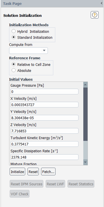
Initialize the solution. You may need to patch a high-temperature region to ignite the flame.
Solution →
Initialization → Initialize
Solution →
Initialization
→ Patch...
Run the solution.
Solution → Run Calculation
Solve the problem and perform postprocessing.
Important: A good initial condition can reduce the solution time substantially. You should start from an existing solution calculated using the Laminar Finite-Rate, EDC model, non-premixed combustion model, or partially premixed combustion model. See Modeling Species Transport and Finite-Rate Chemistry, Modeling Non-Premixed Combustion, and Modeling Partially Premixed Combustion for further information on such simulations.
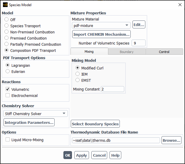
To enable the composition PDF transport model, select Composition PDF Transport in the Species Model dialog box (Figure 19.34: The Species Model Dialog Box for Lagrangian Composition PDF Transport).
![]() Setup → Models → Species
Setup → Models → Species ![]() Edit...
Edit...
When you enable Composition PDF Transport, the dialog box will expand to show the relevant inputs.
Select Lagrangian under PDF Transport Options.
Enable Volumetric under Reactions.
The Composition Pdf Transport model uses Ansys Fluent stiff chemistry solver with ISAT enabled by default. See Using ISAT for more details.
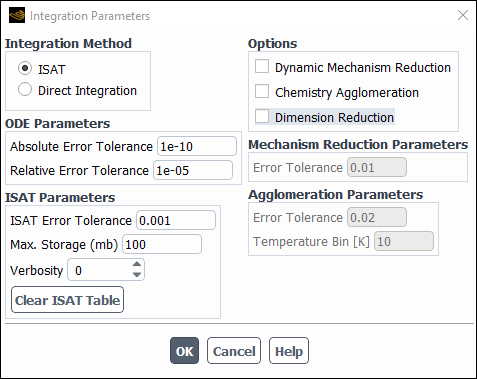
Click the button to open the Integration Parameters Dialog Box (Figure 19.35: The Integration Parameters Dialog Box). For additional information, see Using ISAT.
Enable Liquid Micro-Mixing to interpolate
 from turbulence models
and scalar spectra, as noted in Liquid Reactions in the Theory Guide. This is
applied to cases where reactions in liquids occur at low turbulence
levels, among reactants with low diffusivities. Therefore, a default
value of
from turbulence models
and scalar spectra, as noted in Liquid Reactions in the Theory Guide. This is
applied to cases where reactions in liquids occur at low turbulence
levels, among reactants with low diffusivities. Therefore, a default
value of  may not be desirable, as it over-estimates
the mixing rate.
may not be desirable, as it over-estimates
the mixing rate.In the Mixing tab, select Modified Curl, IEM, or EMST under Mixing Model and specify the value of the Mixing Constant (
 in Equation 7–153 in the Theory Guide). For more
information about particle diffusion, see Particle Mixing in the Theory Guide.
in Equation 7–153 in the Theory Guide). For more
information about particle diffusion, see Particle Mixing in the Theory Guide.Important: If the Liquid Micro-Mixing option is enabled, you cannot set the Mixing Constant.
You will not be specifying species boundary conditions in the Boundary tab. This is only applicable to the Eulerian PDF Transport Option.
In the Control tab, you will specify the Lagrangian PDF transport control parameters.
- Particles Per Cell
sets the number of PDF particles per cell. Higher values of this parameter will reduce statistical error, but increase computational time.
- Local Time Stepping
is available for steady-state simulations and can increase the convergence rate by taking maximum allowable time-steps on a cell-by-cell basis. (see Equation 7–151 of the Theory Guide). If Local Time Stepping is enabled, then you can specify the following parameters:
- Convection #
specifies the particle convection number (see
 in Equation 7–151 in the Theory Guide).
- Diffusion #
specifies the particle diffusion number (see
 in Equation 7–151).
- Mixing #
specifies the particle mixing number (see
 in Equation 7–151).
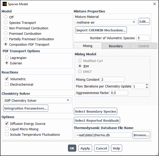
To enable the composition PDF transport model, select Composition PDF Transport in the Species Model dialog box (Figure 19.34: The Species Model Dialog Box for Lagrangian Composition PDF Transport).
![]() Setup → Models → Species
Setup → Models → Species ![]() Edit...
Edit...
When you enable Composition PDF Transport, the dialog box will expand to show the relevant inputs.
Select Eulerian under PDF Transport Options.
Enable Volumetric under Reactions. The Stiff Chemistry Solver is disabled by default and should be enabled if the kinetic mechanism is numerically stiff.
Click the button to open the Integration Parameters Dialog Box (Figure 19.35: The Integration Parameters Dialog Box). See Using ISAT for detailed information about this dialog box.
Make sure that Diffusion Energy Source is enabled if you want to include species diffusion effects in the energy equation.
Enable Liquid Micro-Mixing if the fuel and oxidizer are liquids with low diffusivities (high Schmidt numbers). In this case, the Mixing Constant will be calculated according to Equation 7–160 in the Theory Guide.
By default, the Laminar (one mode) energy equation is solved, where temperature fluctuations are ignored. By enabling Include Temperature Fluctuations, the multi-mode energy equation will be solved as done for species.
In the Mixing tab, only the IEM mixing model is available for Eulerian PDF transport.
Specify the value of the Mixing Constant. The default value is
2for gas phase species.Important: If the Liquid Micro-Mixing option is enabled, you cannot set the Mixing Constant.
Enter the number of Flow Iterations per Chemistry Update. This is the frequency at which Ansys Fluent will update the chemistry during the calculation. Increasing the number can reduce the computational expense of the chemistry calculations.
Enter the Aggressiveness Factor. This is a numerical factor that controls the robustness and the convergence speed. This value ranges between 0 and 1, where 0 is the most robust, but results in the slowest convergence. The default value for the Aggressiveness Factor is 0.5.
In the Boundary tab, define the compositions of the fuel and oxidizer. You can select the boundary species to be displayed as described in Overview of the Problem Setup Procedure.
(Eulerian PDF Transport only) Optionally, you can select the monitored species as described in Overview of the Problem Setup Procedure.
For additional information, see the following sections:
At flow inlets, specify the Mixture Fraction in the Species tab of the boundary condition inlet dialog boxes, as shown in Figure 19.37: The Velocity Inlet Dialog Box for Eulerian Composition PDF Transport. At outlet boundaries, similarly specify the Backflow Mixture Fraction. Ansys Fluent always applies zero flux boundary conditions at walls for all species.
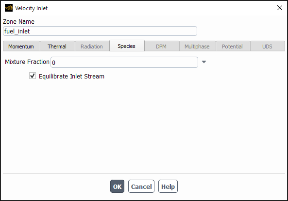
The Equilibrate Inlet Stream option in the Species tab of the boundary conditions dialog boxes will set the inlet compositions to their chemical equilibrium values. This option can be used to model pilot flames and exhaust gas recirculation.
Important: This option should not be enabled for pure fuel or oxidizer inlets.
If you are using the Eulerian PDF transport model, specify the discretization and under-relaxation for the Eulerian PDF composition transport in the Solution Controls and Solution Methods task page.
For the Eulerian PDF Transport model, the initialization variables are the mixture fraction and the temperature. The species mass fractions and enthalpy are calculated based on the fuel and oxidizer composition (specified in the Species dialog box) and the initialized mixture fraction and temperature.
At low speeds, combustion couples to the fluid flow through density. The Lagrangian PDF transport algorithm has random fluctuations in the density field, which in turn causes fluctuations in the flow field. For steady-state flows, statistical fluctuations are decreased by averaging over a number of previous iterations in the Run Calculation task page (Figure 19.39: The Run Calculation Task Page for Composition PDF Transport).
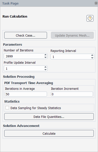
Averaging reduces statistical fluctuations and stabilizes the solution. However, Ansys Fluent often indicates convergence of the flow field before the composition fields (temperatures and species) are converged. You should lower the default convergence criteria in the Residual Monitors Dialog Box, and always check that the Total Heat Transfer Rate in the Flux Reports Dialog Box is balanced. It is also recommended that you monitor temperature/species on outlet boundaries and ensure that these are steady.
The Lagrangian PDF method has the following additional solution controls: Iterations in Average and Iteration Increment. By increasing the Iterations in Average, fluctuations are smoothed out and residuals level off at smaller values. However, the composition PDF method requires a larger number of iterations to reach steady-state. It is recommended that you use the default of 50 Iterations in Average until the steady-state solution is obtained. Then, to gradually decrease the residuals, increase the Iterations in Average by setting a Iteration Increment to a value from 0 to 1 (the value 0.2 is recommended). Subsequent iterations will increase the Iterations in Average by the Iteration Increment.
For additional information, see the following sections:
For unsteady Lagrangian composition PDF transport simulations, a fractional step scheme is employed where the PDF particles are advanced over the time step, and then the flow is advanced over the time step. Unlike steady-state simulations, composition statistics are not averaged over iterations, and to reduce statistical error you should increase the number of particles per cell in the Solution Monitors dialog box.
For low speed flows, the thermo-chemistry couples to the flow through density. Statistical errors in the calculation of density may cause convergence difficulties between time step iterations. If you experience this, increase the number of PDF particles per cell, or decrease the density under-relaxation.
Compressibility is included when ideal-gas is selected as the density method in the Create/Edit Materials Dialog Box. For such flows, particle
internal energy is increased by  over the time step
  , where
  is the cell pressure and
  is the change in the particle specific volume over
the time step.
is the change in the particle specific volume over
the time step.
When solid zones are present in the simulation, Ansys Fluent solves the energy equation in the turbulent flow zones by the Lagrangian Monte Carlo particle method, and the energy equation in the solid zones by the finite-volume method.
For additional information, see the following sections:
Ansys Fluent provides several reporting options for the Lagrangian composition PDF transport calculations. You can generate graphical plots or alphanumeric reports of the following items:
Static Temperature
Mean Static Temperature
RMSE Static Temperature
Mass fraction of species-n
Mean species-n Mass Fraction
RMS species-n Mass Fraction
The instantaneous composition (Static Temperature and Mass fraction of species-n) in a cell are calculated as,
 | (19–13) |
| where | |
|
| |
|
| |
|
| |
|
|


Mean and root-mean-square-error (RMSE) temperatures are calculated in Ansys Fluent by averaging instantaneous temperatures over a user-specified number of previous iterations (see Monitoring the Solution).
Note that for steady-state simulations, instantaneous temperatures and species represent a Monte Carlo realization and are as such unphysical. Mean and RMSE quantities are much more useful.
When you have enabled the Lagrangian composition PDF transport model, you can display the trajectories of the PDF particles using the Particle Tracks Dialog Box (Figure 19.40: The Particle Tracks Dialog Box for Tracking PDF Particles).
![]() Results → Graphics →
Particle Tracks
Results → Graphics →
Particle Tracks
![]() New...
New...
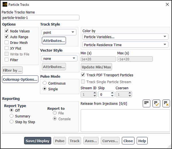
Select the Track PDF Transport Particles option to enable PDF particle tracking. To speed up the plotting
process, you can specify a value  for Skip, which will plot only every
  th particle. For details
about setting other parameters in the Particle Tracks dialog box, see Displaying of Trajectories.
th particle. For details
about setting other parameters in the Particle Tracks dialog box, see Displaying of Trajectories.
When you have finished setting parameters, click to display the particle trajectories in the graphics window.
For additional information, see the following sections: