


For additional information, see the following sections:
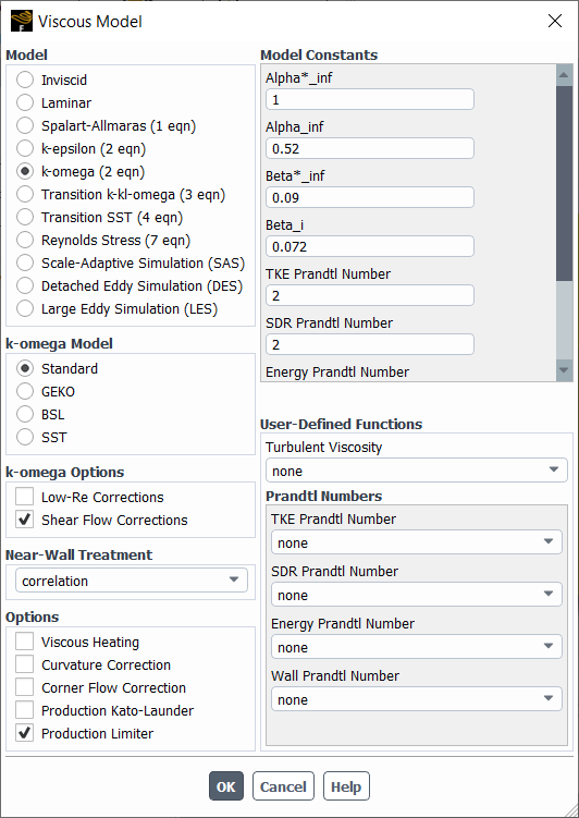
If you choose the standard  -
- model, the following options are available:
low-Re corrections (Low-Re Corrections)
shear flow corrections (Shear Flow Corrections)
turbulence damping (available with the VOF and Mixture models and the Eulerian multiphase model when using the Multi-Fluid VOF model) (Turbulence Damping)
near wall treatment (y+-Insensitive Near-Wall Treatment for ω-based Turbulence Models in the Fluent Theory Guide)
viscous heating (always enabled for the density-based solvers) (Including the Viscous Heating Effects)
inclusion of curvature correction (Including the Curvature Correction for the Spalart-Allmaras and Two-Equation Turbulence Models)
inclusion of compressibility effects (Including the Compressibility Effects Option)
inclusion of production limiters (Including Production Limiters for Two-Equation Models)
a scale-resolving simulation option: Scale-Adaptive Simulation (Setting Up Scale-Adaptive Simulation (SAS) Modeling)
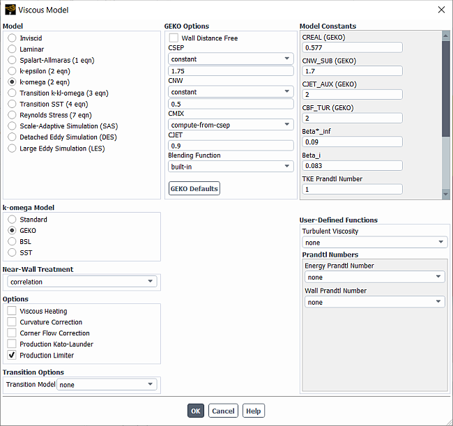
To enable the GEKO turbulence model, you must select the k-omega (2 eqn) model on the Viscous Model dialog box and then select GEKO in the k-omega Model group box.
If you choose the GEKO  -
- model, the following options are available:
turbulence damping (available with the VOF and Mixture models and the Eulerian multiphase model when using the Multi-Fluid VOF model) (Turbulence Damping)
near wall treatment (y+-Insensitive Near-Wall Treatment for ω-based Turbulence Models in the Fluent Theory Guide)
viscous heating (always enabled for the density-based solvers) (Including the Viscous Heating Effects)
inclusion of curvature correction (Including the Curvature Correction for the Spalart-Allmaras and Two-Equation Turbulence Models)
inclusion of compressibility effects (Including the Compressibility Effects Option)
inclusion of production limiters (Including Production Limiters for Two-Equation Models)
inclusion of the Intermittency Transition model
scale-resolving simulation options: either Scale-Adaptive Simulation (Setting Up Scale-Adaptive Simulation (SAS) Modeling), Detached Eddy Simulation (Setting Up DES with the Transition SST Model), Stress-Blended Eddy Simulation (Including the SDES or SBES Model with RANS Models), or Shielded Detached Eddy Simulation (Including the SDES or SBES Model with RANS Models).
If you intend to combine the GEKO model with a Reynolds Stress Model, you must first select the Reynolds Stress Model based on BSL equation (Stress-BSL). You can then enable the GEKO option in the Options group box of the Viscous Model dialog box.
In most cases, you would only tune the coefficients  and
and  .
.
Optimize the coefficient
 for the separation characteristics of wall boundary
layers, which in most applications has the strongest impact on
performance.
for the separation characteristics of wall boundary
layers, which in most applications has the strongest impact on
performance.Adjust
 to affect the mixing behavior of free shear flows (free
mixing layers, etc.).
to affect the mixing behavior of free shear flows (free
mixing layers, etc.).
For more details regarding these coefficients, see Generalized k-ω (GEKO) Model and Generalized k-ω (GEKO) Model in the Fluent Theory Guide.
As these coefficients are both available through expressions and UDF, you can also adjust them differently in different parts of the domain. The other two parameters can, in most cases, be left to their default settings.
By default, the full model is enabled and gives access to all model coefficients and the blending function in the GEKO Options group box (Figure 15.11: The Viscous Model Dialog Box with GEKO Options for the Full Model ). For the wall distance free model option, only a subset of model coefficients can be used.
The corresponding text command to enable the GEKO turbulence model is
/define/models/viscous/kw-geko?
For combination with Reynolds stress models you must first enable the corresponding Reynolds Stress Model and then use the TUI command.
/define/models/viscous/rsm-or-earsm-geko-option?
After GEKO is enabled, all model coefficients and the blending function are
available in the submenu geko-options:
/define/models/viscous/geko-options/wall-distance-free?
/define/models/viscous/geko-options/csep
/define/models/viscous/geko-options/cnw
/define/models/viscous/geko-options/cmix
/define/models/viscous/geko-options/cjet
/define/models/viscous/geko-options/blending-function
The auxiliary coefficients are also available as TUI commands.
/define/models/viscous/geko-options/creal
/define/models/viscous/geko-options/cnw_sub
/define/models/viscous/geko-options/cjet_aux
/define/models/viscous/geko-options/cbf_lam
/define/models/viscous/geko-options/cbf_tur
Furthermore, it is possible to reset these model parameters to default values by clicking GEKO Defaults or the TUI command:
/define/models/viscous/geko-options/geko-defaults
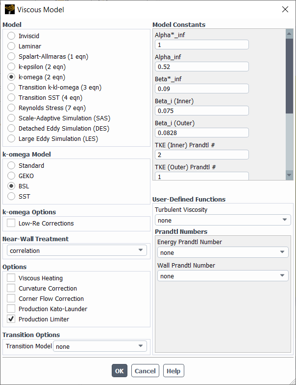
If you choose the baseline (BSL)  -
- model, the following options are available:
low-Re corrections (Low-Re Corrections)
turbulence damping (available with the VOF and Mixture models and the Eulerian multiphase model when using the Multi-Fluid VOF model) (Turbulence Damping)
near wall treatment (y+-Insensitive Near-Wall Treatment for ω-based Turbulence Models in the Fluent Theory Guide)
viscous heating (always enabled for the density-based solvers) (Including the Viscous Heating Effects)
inclusion of curvature correction (Including the Curvature Correction for the Spalart-Allmaras and Two-Equation Turbulence Models)
inclusion of compressibility effects (Including the Compressibility Effects Option)
inclusion of production limiters (Including Production Limiters for Two-Equation Models)
inclusion of the Intermittency Transition model
scale-resolving simulation options: either Scale-Adaptive Simulation (Setting Up Scale-Adaptive Simulation (SAS) Modeling), Detached Eddy Simulation (Setting Up DES with the Transition SST Model), Stress-Blended Eddy Simulation (Including the SDES or SBES Model with RANS Models), or Shielded Detached Eddy Simulation (Including the SDES or SBES Model with RANS Models).
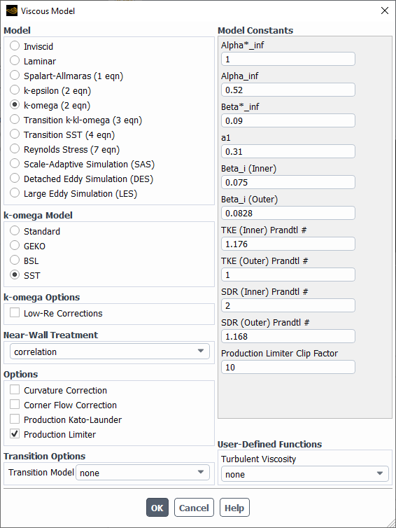
If you choose the shear-stress transport - model, the following
options are available:
low-Re corrections (Low-Re Corrections)
turbulence damping (available with the VOF and Mixture models and the Eulerian multiphase model when using the Multi-Fluid VOF model) (Turbulence Damping)
near wall treatment (y+-Insensitive Near-Wall Treatment for ω-based Turbulence Models in the Fluent Theory Guide)
viscous heating (always enabled for the density-based solvers) (Including the Viscous Heating Effects)
inclusion of curvature correction (Including the Curvature Correction for the Spalart-Allmaras and Two-Equation Turbulence Models)
inclusion of compressibility effects (Including the Compressibility Effects Option)
inclusion of production limiters (Including Production Limiters for Two-Equation Models)
inclusion of the Intermittency Transition model
scale-resolving simulation options: Stress-Blended Eddy Simulation or Shielded Detached Eddy Simulation (Including the SDES or SBES Model with RANS Models).
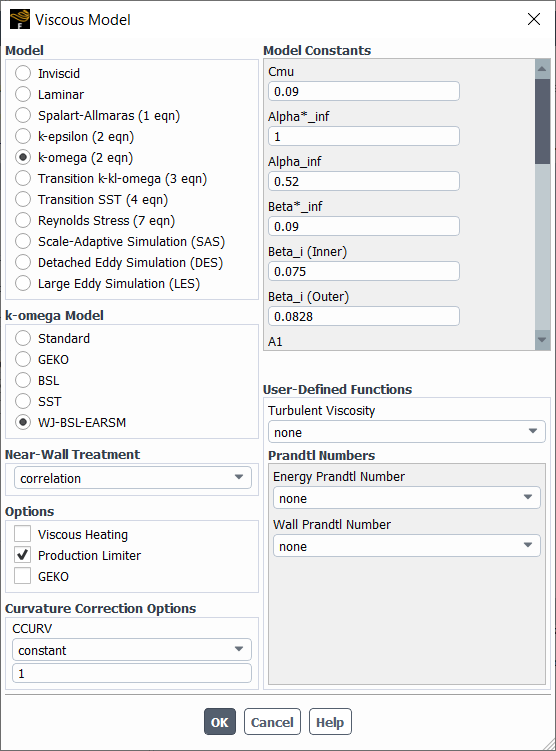
If you choose the WJ-BSL-EARSM
- model, the following options are available:
near wall treatment (y+-Insensitive Near-Wall Treatment for ω-based Turbulence Models in the Fluent Theory Guide)
viscous heating (always enabled for the density-based solvers) (Including the Viscous Heating Effects)
inclusion of production limiters (Including Production Limiters for Two-Equation Models)
enabling the GEKO model in combination with the WJ-BSL-EARSM by selecting GEKO under Options.(Setting up the Generalized k-ω (GEKO) Model)
inclusion of curvature correction (Including the Curvature Correction for the Spalart-Allmaras and Two-Equation Turbulence Models)
The model is available when the k-omega model is selected. The WJ-BSL-EARSM option becomes available under k-omega Model, as shown in Figure 15.14: The Viscous Model Dialog Box With WJ-BSL-EARSM Enabled.
Note: It is only available for 3D cases, and is not supported with the gap model.
The WJ-BSL-EARSM is an extension of the Baseline
(BSL) - model and allows to capture the following flow effects:
Anisotropy of Reynolds Stresses
Secondary Flows