


This section provides details about the non-premixed combustion modeling capabilities in Ansys Fluent.
The non-premixed combustion model is presented in the following sections:
- 20.1.1. Steps in Using the Non-Premixed Model
- 20.1.2. Setting Up the Equilibrium Chemistry Model
- 20.1.3. Setting Up the Steady and Unsteady Diffusion Flamelet Models
- 20.1.4. Defining the Stream Compositions
- 20.1.5. Setting Up Control Parameters
- 20.1.6. Calculating the Flamelets
- 20.1.7. Calculating the Look-Up Tables
- 20.1.8. Standard Files for Diffusion Flamelet Modeling
- 20.1.9. Setting Up the Inert Model
- 20.1.10. Defining Non-Premixed Boundary Conditions
- 20.1.11. Defining Non-Premixed Physical Properties
- 20.1.12. Solution Strategies for Non-Premixed Modeling
- 20.1.13. Enabling Robust Numerics for Combustion with a PDF Table
- 20.1.14. Postprocessing the Non-Premixed Model Results
For theoretical background on the non-premixed combustion model, see Non-Premixed Combustion in the Theory Guide.
A description of the inputs for the non-premixed model is provided in the sections that follow.
Before turning on the non-premixed combustion model, you must enable turbulence calculations in the Viscous Model Dialog Box.
![]() Setup → Models → Viscous
Setup → Models → Viscous ![]() Edit...
Edit...
If your model is non-adiabatic, you should also enable heat transfer (and radiation, if required).
![]() Setup → Models → Energy
Setup → Models → Energy ![]() ON
ON
![]() Setup → Models → Radiation
Setup → Models → Radiation ![]() Edit...
Edit...
Figure 8.7: Reacting Systems Requiring Non-Adiabatic Non-Premixed Model Approach in the Theory Guide illustrates the types of problems that must be treated as non-adiabatic.
Your first task is to define the type of reaction system and reaction model that you intend to use. This includes selection of the following options:
Non-premixed or partially premixed model option (see Modeling Partially Premixed Combustion).
Equilibrium chemistry model, steady diffusion flamelet model, unsteady diffusion flamelet model, or diesel unsteady flamelet.
Adiabatic or non-adiabatic modeling options (see Non-Adiabatic Extensions of the Non-Premixed Model in the Theory Guide).
Addition of a secondary stream (equilibrium model only).
Empirically defined fuel and/or secondary stream composition (equilibrium model only).
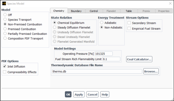
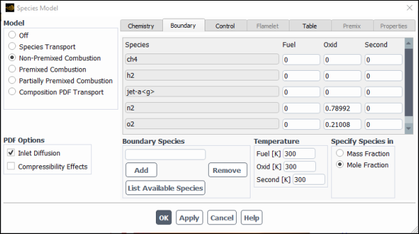
You can make these model selections using the Species Model dialog box (Figure 20.6: The Species Model Dialog Box (Chemistry Tab)).
![]() Setup → Models → Species
Setup → Models → Species ![]() Edit...
Edit...
For a single-mixture-fraction problem, you will perform the following steps:
Choose the chemical description of the system: chemical equilibrium, steady diffusion flamelet, unsteady diffusion flamelet, or diesel unsteady flamelet (Figure 20.1: Defining Equilibrium Chemistry).
Indicate whether the problem is adiabatic or non-adiabatic.
(steady diffusion flamelet model only) Import a flamelet file or appropriate CHEMKIN mechanism file if generating flamelets (Figure 20.2: Defining Steady Diffusion Flamelet Chemistry).
Define the chemical boundary species to be considered for the streams in the reacting system model. Note that this step is not relevant in the case of flamelet import (Figure 20.3: Defining Chemical Boundary Species). For more information, see Defining the Stream Compositions.
(steady diffusion flamelet model only) If you are generating flamelets, compute the flamelet state relationships of species mass fractions, density, and temperature as a function of mixture fraction and scalar dissipation (Figure 20.4: Calculating Steady Diffusion Flamelets).
Compute the final chemistry look-up table, containing mean values of species fractions, density, and temperature as a function of mean mixture fraction, mixture fraction variance, and possibly enthalpy and scalar dissipation. The contents of this look-up table will reflect your preceding inputs describing the turbulent reacting system (Figure 20.5: Calculating the Chemistry Look-Up Table).
The look-up table is the stored result of the integration of Equation 8–17 (or Equation 8–25) and Equation 8–19 (in the Theory Guide). The look-up table will be used in Ansys Fluent to
determine mean species mass fractions, density, and temperature from the values of mean mixture
fraction ( ), mixture fraction variance (
 ), and possibly mean enthalpy (
 ) and mean scalar dissipation (
 ) as they are computed during the Ansys Fluent calculation of the reacting flow.
See Look-Up Tables for Adiabatic Systems and Figure 8.8: Visual Representation of a Look-Up Table for the Scalar (Mean
Value of Mass Fractions, Density, or Temperature) as a Function of
Mean Mixture Fraction and Mixture Fraction Variance in Adiabatic Single-Mixture-Fraction
Systems and Figure 8.10: Visual Representation of a Look-Up Table for the Scalar as
a Function of Mean Mixture Fraction and Mixture Fraction Variance
and Normalized Heat Loss/Gain in Non-Adiabatic Single-Mixture-Fraction
Systems in the Theory Guide.
) as they are computed during the Ansys Fluent calculation of the reacting flow.
See Look-Up Tables for Adiabatic Systems and Figure 8.8: Visual Representation of a Look-Up Table for the Scalar (Mean
Value of Mass Fractions, Density, or Temperature) as a Function of
Mean Mixture Fraction and Mixture Fraction Variance in Adiabatic Single-Mixture-Fraction
Systems and Figure 8.10: Visual Representation of a Look-Up Table for the Scalar as
a Function of Mean Mixture Fraction and Mixture Fraction Variance
and Normalized Heat Loss/Gain in Non-Adiabatic Single-Mixture-Fraction
Systems in the Theory Guide.
For a problem that includes a secondary stream (and, therefore, a second mixture fraction), you will perform the first two steps listed above for the single-mixture-fraction approach and then prepare a look-up table of instantaneous properties using Equation 8–13 or Equation 8–15 in the Theory Guide.
In the equilibrium chemistry model, the concentrations of species of interest are determined from the mixture fraction using the assumption of chemical equilibrium (see Non-Premixed Combustion and Mixture Fraction Theory in the Theory Guide). With this model, you can include the effects of intermediate species and dissociation reactions, producing more realistic predictions of flame temperatures than the Eddy-Dissipation model. When you choose the equilibrium chemistry option, you will have the opportunity to use the rich flammability limit (RFL) option.
To enable the equilibrium chemistry model
Select Non-Premixed Combustion in the Species Model dialog box.
Select Chemical Equilibrium in the Chemistry tab of the Species Model dialog box.
For additional information, see the following sections:
You should use the non-adiabatic modeling option if your problem definition in Ansys Fluent will include one or more of the following:
radiation or wall heat transfer
multiple fuel inlets at different temperatures
multiple oxidant inlets at different temperatures
liquid fuel, coal particles, and/or heat transfer to inert particles
Note that the adiabatic model is a simpler model involving a
two-dimensional look-up table in which scalars depend only on  and
and  (or on
  and
and  ).
If your model is defined as adiabatic, you will not need to solve
the energy equation in Ansys Fluent and the system temperature will be
determined directly from the mixture fraction and the fuel and oxidant
inlet temperatures. The non-adiabatic case will be more complex and
more time-consuming to compute, requiring the generation of three-dimensional
look-up tables. However, the non-adiabatic model option allows you
to include the types of reacting systems described above.
).
If your model is defined as adiabatic, you will not need to solve
the energy equation in Ansys Fluent and the system temperature will be
determined directly from the mixture fraction and the fuel and oxidant
inlet temperatures. The non-adiabatic case will be more complex and
more time-consuming to compute, requiring the generation of three-dimensional
look-up tables. However, the non-adiabatic model option allows you
to include the types of reacting systems described above.
Select Adiabatic or Non-Adiabatic in the Chemistry tab of the Species Model dialog box.
The system Operating Pressure is used to calculate density using the ideal gas law. For non-adiabatic simulations, the Compressibility Effects under PDF Options can be enabled to account for cases where substantial pressure changes occur in time and/or space. In such cases it is assumed that the species mass fractions do not change with pressure, and the density is calculated as
 | (20–1) |
where  is the density
at the specified Operating Pressure (
is the density
at the specified Operating Pressure ( ), and
  is the local mean pressure in an Ansys Fluent cell.
When the Compressibility Effects option is enabled, the flow operating pressure (set in the Operating Conditions dialog box) can differ from the Non-Premixed model operating pressure. To distinguish this difference, the Operating Pressure name tag in the Species Model dialog box changes to Equilibrium Operating Pressure when the compressibility effects option is enabled.
Note that for the Operating Pressure or Equilibrium Operating Pressure, you should specify a value close to the absolute pressure in the system.
See Solution Strategies for Non-Premixed Modeling for details about enabling compressibility effects.
If you are modeling a system consisting of a single fuel and a single oxidizer stream, you do not need to enable a secondary stream in your PDF calculation. As discussed in Definition of the Mixture Fraction in the Theory Guide, a secondary stream should be enabled if your PDF reaction model will include any of the following:
two dissimilar gaseous fuel streams
In these simulations, the fuel stream defines one of the fuels and the secondary stream defines the second fuel.
mixed fuel systems of dissimilar gaseous and liquid fuel
In these simulations, the fuel stream defines the gaseous fuel and the secondary stream defines the liquid fuel (or vice versa).
mixed fuel systems of dissimilar gaseous and coal fuels
In these simulations, you can use the fuel stream or the secondary stream to define either the coal or the gaseous fuel. See Modeling Coal Combustion Using the Non-Premixed Model regarding coal combustion simulations with the non-premixed combustion model.
mixed fuel systems of coal and liquid fuel
In these simulations, you can use the fuel stream or the secondary stream to define either the coal or the liquid fuel. See Modeling Coal Combustion Using the Non-Premixed Model regarding coal combustion simulations with the non-premixed combustion model.
coal combustion
Coal combustion can be more accurately modeled by using a secondary stream to track the distinct volatile and char off-gases. The fuel stream must define the char and the secondary stream must define the volatile components of the coal. See Modeling Coal Combustion Using the Non-Premixed Model regarding coal combustion simulations with the non-premixed combustion model.
a single fuel with two dissimilar oxidizer streams
In these simulations, the fuel stream defines the fuel, the oxidizer stream defines one of the oxidizers, and the secondary stream defines the second oxidizer.
To include a secondary stream in your model, turn on the Secondary Stream option under Stream Options in the Chemistry tab.
Important: Using a secondary stream can substantially increase the calculation time for your simulation since the multi-dimensional PDF integrations are performed at run time. Alternatively, Ansys Fluent can perform a full tabulation of the PDF integrations, as detailed in Full Tabulation of the Two-Mixture-Fraction Model.
When the secondary stream is present, only instantaneous species mass fraction, temperature and mixture properties are stored inside the PDF table. The probability density function (PDF) calculates averaged species mass fraction and mixture properties at the run time. After a PDF table has been generated or read into Ansys Fluent, you can select the shape of the assumed PDF from the Probability Density Function drop-down list (PDF Options group box):
double delta: as given by Equation 8–21 in the Fluent Theory Guide.
beta: as given by Equation 8–22 in the Fluent Theory Guide.
The empirical fuel option provides an alternative method for defining the composition of the fuel or secondary stream when the individual species components of the fuel are unknown. That is, you will define the elemental fraction not the individual species. When this option is disabled, you will define the chemical species that are present in each stream and the mass or mole fraction of each species, as described in Defining the Stream Compositions. The option for defining an empirical fuel stream is particularly useful for coal combustion simulations (see Modeling Coal Combustion Using the Non-Premixed Model) or for simulations involving other complex hydrocarbon mixtures.
To define a fuel or secondary stream empirically
Turn on the Empirical Fuel Stream option under Stream Options in the Chemistry tab of the Species Model dialog box. If you have a secondary stream, enable the Empirical Secondary Stream option, or both as appropriate.
Specify the appropriate lower heating value (for example Empirical Fuel Lower Caloric Value, Empirical Secondary Lower Caloric Value), specific heat (Empirical Fuel Specific Heat, Empirical Secondary Specific Heat), and molecular weight (Empirical Fuel Molecular Weight, Empirical Secondary Molecular Weight) for each empirically defined stream.
Important: The empirical definition option is available only with the full equilibrium chemistry model. It cannot be used with the rich flammability limit (RFL) option or the steady and unsteady diffusion flamelet models, since equilibrium calculations are required for the determination of the fuel composition.
Important: The empirical fuel and secondary molecular weights are only required if your empirical streams are entering the domain via an inlet boundary, or if you are using the partially premixed model. If you are using the non-premixed model and the empirically defined streams originate from the dispersed phase (for example, if you are modeling coal or liquid fuel combustion) the molecular weights are not required for the computation.
You can define a rich limit on the mixture fraction when the equilibrium chemistry option is used. Input of the rich limit is accomplished by specifying a value of the Rich Flammability Limit for the appropriate Fuel Stream, Secondary Stream, or both. You will not be allowed to specify the Rich Flammability Limit if you have used the empirical definition option for fuel composition.
Ansys Fluent will compute the composition at the rich limit using
equilibrium. For mixture fraction values above this limit, Ansys Fluent will
suspend the equilibrium chemistry calculation and will compute the
composition based on mixing, but not burning, of the fuel with the
composition at the rich limit. A value of 1.0 for the rich limit implies
that equilibrium calculations will be performed over the full range
of mixture fraction. When you use a rich limit that is less than 1.0,
equilibrium calculations are suspended whenever  ,
,  , or
, or  exceeds
the limit. This RFL model is often more accurate than the assumption
of chemical equilibrium for rich mixtures, and also avoids complex
equilibrium calculations, speeding up the preparation of the look-up
tables. An RFL value of approximately twice the stoichiometric mixture
fraction is appropriate.
exceeds
the limit. This RFL model is often more accurate than the assumption
of chemical equilibrium for rich mixtures, and also avoids complex
equilibrium calculations, speeding up the preparation of the look-up
tables. An RFL value of approximately twice the stoichiometric mixture
fraction is appropriate.
For the Secondary Stream, the rich flammability
limit controls the equilibrium calculation for the secondary mixture
fraction. If your secondary stream is not a fuel, you should use an
RFL value of 1. A value of 1.0 for the rich limit implies that equilibrium
calculations will be performed over the full range of mixture fraction.
When you input a rich limit that is less than 1.0, equilibrium calculations
are suspended whenever  exceeds
the limit. (Note that it is the secondary mixture fraction
exceeds
the limit. (Note that it is the secondary mixture fraction  and not the partial fraction
  that is used here.)
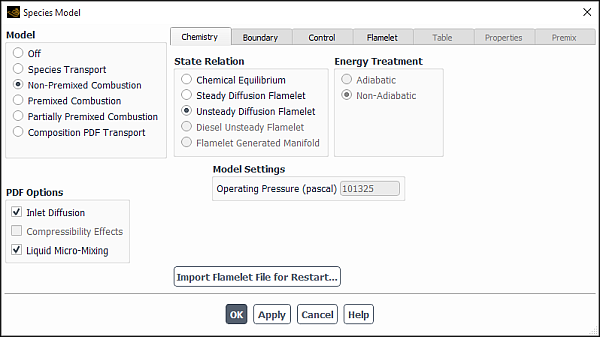
To enable the diffusion flamelet models
Select Non-Premixed Combustion in the Species Model dialog box.
Select Steady Diffusion Flamelet or Unsteady Diffusion Flamelet in the Chemistry tab of the Species Model dialog box. See Using the Unsteady Diffusion Flamelet Model.
For additional information, see the following sections:
- 20.1.3.1. Choosing Adiabatic or Non-Adiabatic Options
- 20.1.3.2. Specifying the Operating Pressure for the System
- 20.1.3.3. Specifying a Chemical Mechanism File for Flamelet Generation
- 20.1.3.4. Importing a Flamelet
- 20.1.3.5. Using the Unsteady Diffusion Flamelet Model
- 20.1.3.6. Using the Diesel Unsteady Laminar Flamelet Model
- 20.1.3.7. Resetting Diesel Unsteady Flamelets
Select Adiabatic or Non-Adiabatic in the Chemistry tab of the Species Model dialog box. See the discussion in Choosing Adiabatic or Non-Adiabatic Options about the two options.
The system Operating Pressure is used to calculate density using the ideal gas law. When the Compressibility Effects option is enabled, the name Operating Pressure is changed to Equilibrium Operating Pressure since the non-premixed combustion model operating pressure can differ from the flow operating pressure. Specifying the Operating Pressure for the System provides more information about this value.
You can use the steady or unsteady diffusion flamelet model for reactions in liquid systems. To do so, enable Liquid Micro-Mixing under PDF Options. The Liquid Micro-Mixing option is discussed in detail in Liquid Reactions in the Theory Guide.
If you are generating a flamelet file yourself, you will need to read in the chemical kinetic mechanism and thermodynamic data. The mechanism and thermodynamic data must be in CHEMKIN format [79].
To read in a CHEMKIN mechanism, select the Create Flamelet option in the Chemistry tab of the Species Model dialog box and click the button. Using the Import CHEMKIN Format Mechanism dialog box, import the gas-phase files into Ansys Fluent as described in Importing a Volumetric Kinetic Mechanism in CHEMKIN Format. Note that for flamelet generation, only a gas-phase kinetic mechanism and a thermodynamic database are required.
Note that the import is limited to mechanisms with 700 or fewer species.
To import an existing flamelet file
Select the Import Flamelet option in the Chemistry tab of the Species Model dialog box.
(steady diffusion flamelet only) Select either Standard or CFX-RIF format under File Type.
Click the button. In The Select File Dialog Box, select the file (for a single flamelet) or files (for multiple flamelets) to be read in to Ansys Fluent.
After you have completed this step, you can skip ahead to the Table tab of the Species Model dialog box (see Calculating the Look-Up Tables).
The unsteady diffusion flamelet model can only be enabled from a valid steady-state, steady diffusion flamelet solution. When enabled, the unsteady diffusion flamelet model will change this case to unsteady and postprocess marker probability equations on the frozen flow field. You should hence ensure that the starting steady-state, steady diffusion flamelet solution is fully converged.
When the Unsteady Diffusion Flamelet is enabled in the Chemistry tab, the button appears in the dialog box, allowing you to run the simulation from a previously saved case, data and unsteady flamelet file.
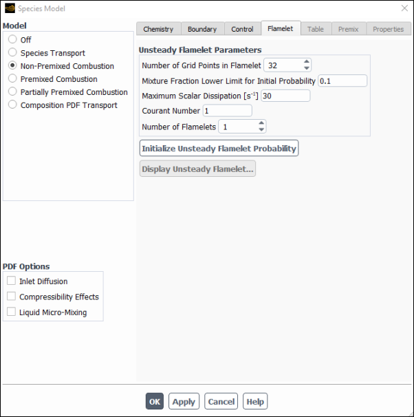
The Unsteady Diffusion Flamelet Model requires four user inputs in the Flamelet tab:
The Number of Grid Points in Flamelet.
The Mixture Fraction Lower Limit for Initial Probability. The initial condition of the marker probability field is unity for all mean mixture fractions above the Mixture Fraction Lower Limit for Initial Probability, and zero for mean mixture fractions below it. Note that this should be specified to be greater than the stoichiometric mixture fraction.
Maximum Scalar Dissipation. Flamelets may extinguish at high scalar dissipations because diffusion in the flamelet overwhelms reaction. It is possible to have unrealistically high modeled scalar dissipation in the 2D or 3D Ansys Fluent simulations, which gets transferred to the 1D unsteady flamelet. In order to avoid excessive diffusion in the 1D unsteady flamelet, the instantaneous scalar dissipation in the 1D flamelet is limited to the specified Maximum Scalar Dissipation.
Courant Number. The time step size for the unsteady probability marker equation is calculated automatically by Ansys Fluent based on the Courant Number. Larger values imply a smaller number of time steps to convect/diffuse the marker probability out of the domain, but also results in a larger numerical error. The Courant Number should be small enough so that the unsteady flamelet mean mass fractions are unchanged with any smaller Courant Number. The default value of 1 should be sufficient for most applications.
Number of Flamelets. The number of unsteady laminar flamelets that Ansys Fluent will generate during the run. The marker probability equation Equation 8–57 in the Fluent Theory Guide will be solved for each flamelet.
When these inputs have been set, clicking the button initializes the marker probability equation for each flamelet, automatically enabling the Unsteady solver, while disabling all equations except the Unsteady Flamelet Probability equation in the Solution Controls task page. This initialization in the Flamelet tab also sets the Time Step Size in the Run Calculation task page.
Important:
Do not initialize your solution from the tree or the Solution Initialization task page. Note that you are postprocessing a probability field on the frozen steady-state flow field, and by clicking the button, you have already initialized the probability marker field.
If you disable the Unsteady Diffusion Flamelet model and you want to revert to solving a steady diffusion flamelet simulation, make sure you enable Steady (either in the General task page or in the tree from the Setup/General/ Analysis Type tree item) and enable all the equations (in the Solution Controls task page or in the tree from the Solution/Solution Controls tree item).
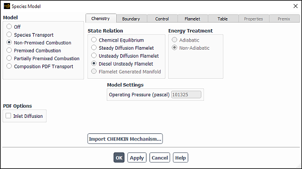
The diesel unsteady laminar flamelet model can only be enabled when conditions for compression-ignition are met:
The Transient solver is selected in the General task page (or in the tree from the Setup/General/ Analysis Type).
The In-Cylinder dynamic mesh is enabled.
The Discrete Phase model option Interaction with Continuous Phase is selected.
The basic steps for setting the diesel unsteady laminar flamelet models are as follows.
In the Chemistry tab, select Diesel Unsteady Flamelet.
If a detailed chemical mechanism containing kinetic reactions appropriate for compression ignition has not yet been defined in your case, you can import a mechanism in CHEMKIN format as described in Importing a Volumetric Kinetic Mechanism in CHEMKIN Format.
The mechanism can include pollutant formation reactions as well if you are interested in modeling emissions.
In the Boundary tab, define the stream compositions as described in Defining the Stream Compositions.
In the Flamelet tab, set the following flamelet parameters.
Set the Number of Grid Points in Flamelet.
Set the Number of Unsteady Flamelets that Ansys Fluent will generate during simulation.
(for multiple unsteady flamelets) Set the flamelet start times.
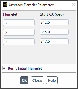
Ansys Fluent automatically sets the start time for the first flamelet, but you must set the start time for each consecutive flamelet using the Unsteady Flamelet Parameters dialog box. Open it by clicking Set Flamelet Parameters and enter the start time for each flamelet either in seconds or in crank angles if the dynamic mesh is enabled.
Ansys Fluent starts simulation with only one flamelet, and then it automatically introduces new flamelets into the reacting domain at the times you have specified.
The default initial condition for an unsteady flamelet is unburnt. Ansys Fluent provides the Burnt Initial Flamelet option that allows you to set the initial flamelet condition to a chemical equilibrium burnt state. This option is useful if you are modeling internal combustion engines where residual gases may be present in the cylinder before the spray is injected, which would be incorrectly modeled by the unburnt state. Note that the Burnt Initial Flamelet is only used at case initialization.
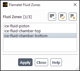
(optional) Specify the flamelet fluid zones.
Ansys Fluent calculates diesel unsteady flamelets using the zone-averaged pressure and scalar dissipation at every time step. By default, the averaging is performed over all fluid zones in the domain, but you can also select and/or deselect the fluid zones using the Flamelet Fluid Zones dialog box. Open this dialog box by clicking Set Flamelet Fluid Zones and select the fluid zones to be used for calculating average pressure and scalar dissipation. If no fluid zone is selected, Ansys Fluent will compute domain average pressure and scalar dissipation using all fluid zones.
Note: For internal combustion cases, it is recommended that you select the cylinder fluid zones and deselect the intake and exhaust fluid zones.
Note that Ansys Fluent calculates flamelets at every time step of the run. For this reason, the option to calculate the flamelets as a preprocessing step before running your simulation is unavailable, and Calculate Flamelets appears dimmed.
In the Table tab, set the PDF table parameters as described in Calculating the Look-Up Tables.
Note that Ansys Fluent calculates the PDF table at every time step of the run. For this reason, the option to calculate the PDF table as a preprocessing step before running your simulation is unavailable, and Calculate PDF Table appears dimmed.
When setting up and using the Diesel Unsteady Flamelet model for internal combustion engine simulations, the following recommendations apply:
Number of Flamelets
You must specify at least two diesel unsteady flamelets. Ansys Fluent will use the first flamelet to model trapped burnt gases from the previous cycle. The second flamelet will start at the crank angle (CA) of fuel injection, specified in the Unsteady Flamelet Parameters dialog box (see Figure 20.10: The Flamelet Fluid Zones Dialog Box).
To model split injections where an initial fuel mass is injected and burns before the main fuel injection, three or more unsteady flamelets are required.
Flamelet Initialization
By default, the flamelet is initialized as mixed-but-unburnt. However, in all practical scenarios there is always some trapped gas remaining inside the cylinder. Therefore, it is recommended that you use the Burnt Initial Flamelet option in the Unsteady Flamelet Parameters dialog box (see Figure 20.10: The Flamelet Fluid Zones Dialog Box). When this option is selected, Ansys Fluent performs a constant temperature equilibrium calculation and sets the initial flamelet condition to a chemical equilibrium burnt state.
Multi-cycle simulations
To accurately model multiple cycles of internal combustion engines, the flamelets must be reset at the end of each cycle. This is performed by defining the Diesel Unsteady Flamelet Reset event, typically at the specified crank angle, just before the inlet valve opens. Refer to the Resetting Diesel Unsteady Flamelets for details. This approach is recommended for modeling the EGR trapped gases with the first burnt unsteady flamelet.
If you are using the Inert (EGR) model in order to track the trapped inert mixture, you need to define the Inert EGR Reset event at the specified crank angle just before the inlet valve opens. See Resetting Inert EGR for details.
In order to simulate multiple cycles in internal combustion engines, flamelets should be reset at the end of every cycle. In addition, the burned trapped gases must be modeled, which can be done in one of the two ways. The first and recommended approach is to use the Diesel Unsteady Flamelet Reset option. The second approach is to use the inert (EGR) model and the Inert EGR Reset option. You can access the Diesel Unsteady Flamelet Reset and Inert EGR Reset options via the Dynamic Mesh Events dialog box. There, you need to set the crank angle at which this event occurs (usually shortly before the inlet valves open) and the participating fluid zones (usually only the combustion chamber and not the intake and exhaust port zones).
When the Diesel Unsteady Flamelet Reset event is executed, all flamelets are deleted and a new flamelet is introduced with a state set to the probability-weighted average condition of all flamelets present before reset. The other new flamelets are introduced during a new cycle in a similar fashion to that described in Using the Diesel Unsteady Laminar Flamelet Model.
When the inert EGR reset event is executed with the diesel unsteady flamelet model, the burnt gas in the selected Inert EGR Reset zones is converted to inert, all flamelets are deleted, and a new unburnt flamelet is introduced into the domain.
Note: The Diesel Unsteady Flamelet Reset option is available only when the selected number of flamelets is greater than one.
In modeling a non-premixed combustion problem, you will only specify the boundary species (that is, the fuel, oxidizer, and if necessary, secondary stream species). The intermediate and product species will be determined automatically.
Ansys Fluent provides you with an initial list of common boundary
species (ch4, h2, jet-a<g>, n2 and o2). If your fuel and/or oxidizer is
composed of different species, you can add them to the boundary Species list. All boundary species must exist in the chemical
database and you must enter their names in the same format used in
the database, otherwise an error message will be issued.
After defining the boundary species that will be considered in the reaction system, you must define their mole or mass fractions at the fuel and oxidizer inlets and at the secondary inlet, if one exists. (If you choose to define the fuel or secondary stream composition empirically, you will instead enter the parameters described at the end of this section.) For the example shown in Figure 8.12: Chemical Systems That Can Be Modeled Using a Single Mixture Fraction in the Theory Guide, for example, the fuel inlet consists of 60% CO4, 20% CO, 10% CO2, and 10% C3H8.
Finally, the inlet stream temperatures of your reacting system are required for construction of the look-up table and computation of the equilibrium chemistry model.
For the equilibrium chemistry model, the species names are entered using the Boundary tab in the Species Model dialog box (Figure 20.11: The Species Model Dialog Box (Boundary Tab)). If you are generating a steady or unsteady diffusion flamelet, the list of boundary species will be automatically filled as all the species in the CHEMKIN mechanism, and you will be unable to change these.
The steps for adding new species and defining their compositions are as follows:
(chemistry equilibrium chemistry model only) If your fuel, oxidizer, or secondary streams are composed of species other than the default species list, type the chemical formula (for example,
so2orSO2for SO ) under Boundary Species and click . The species will be added to the Species list. Continue in this manner until all of the boundary species you want to include are shown in the Species list.
To remove a species from the list, type the chemical formula under Boundary Species and click . To print a list of all species in the thermodynamic database file (
thermo.db) in the console window, click .(non-equilibrium chemistry models) Optionally, select the boundary species as described in Overview of the Problem Setup Procedure.
Under Specify Species In, specify whether you want to enter the Mass Fraction or Mole Fraction. Mass Fraction is the default.
For each relevant species in the Species list, specify its mass or mole fraction for each stream (Fuel, Oxid, or Second as appropriate) by entering values in the table. Note that if you change from Mass Fraction to Mole Fraction (or vice versa), all values will be automatically converted if they sum to 0 or 1, so be sure that you are entering either all mass fractions or all mole fractions as appropriate. If the values do not sum to 0 or 1, an error will be issued.
Under Temperature, specify the following inputs:
- Fuel
is the temperature of the fuel inlet in your model. In adiabatic simulations, this input (together with the oxidizer inlet temperature) determines the inlet stream temperatures that will be used by Ansys Fluent. In non-adiabatic systems, this input should match the inlet thermal boundary condition that you will use in Ansys Fluent (although you will enter this boundary condition again in the Ansys Fluent session). If your Ansys Fluent model will use liquid fuel or coal combustion, define the inlet fuel temperature as the temperature at which vaporization/devolatilization begins (that is, the Vaporization Temperature specified for the discrete-phase material—see Setting Material Properties for the Discrete Phase). For such non-adiabatic systems, the inlet temperature will be used only to adjust the look-up table grid (for example, the discrete enthalpy values for which the look-up table is computed). Note that if you have more than one fuel inlet, and these inlets are not at the same temperature, you must define your system as non-adiabatic. In this case, you should enter the fuel inlet temperature as the value at the dominant fuel inlet.
- Oxid
is the temperature of the oxidizer inlet in your model. The issues raised in the discussion of the input of the fuel inlet temperature (directly above) pertain to this input as well.
- Second
is the temperature of the secondary stream inlet in your model. (This item will appear only when you have defined a secondary inlet.) The issues raised in the discussion of the input of the fuel inlet temperature (directly above) pertain to this input as well.
For additional information, see the following sections:
In combustion, a large number of intermediate and product species may be produced from a small number of initial boundary species. In Ansys Fluent you must specify only the species composition of your boundary species in the fuel, oxidizer, and (if appropriate) secondary streams. Ansys Fluent will calculate all intermediate and product species automatically. The following suggestions may be helpful in the definition of the system chemistry:
For coal combustion, char in the coal should be represented by C(s).
Important: Care should be taken to distinguish atomic carbon, C, from solid carbon, C(s). Atomic carbon should be selected only if you are using the empirically-defined input method.
If your fuel composition is known empirically (for example, C0.9 H3 O0.2), use the option for an empirically-defined stream (see below).
If you want to include the sulfur that may be present in a hydrocarbon fuel, note that this may hinder the convergence of the equilibrium solver, especially if the concentration of sulfur is small. It is therefore recommended that you include sulfur in the calculation only if it is present in considerable quantities.
In addition to gaseous species, liquid and solid species can be included in the chemistry
calculations. They are often indicated by an “l” or an “s” in
parentheses after the species name. If you add a condensed species to the equilibrium chemical
system, its density will be retrieved from Ansys Fluent’s chemical property database file
propdb.scm if you are using the thermodynamic database file
thermo.db that is also supplied with Ansys Fluent. If you are using a
custom thermodynamic database file and want to include a condensed species in the equilibrium
system that does not exist in propdb.scm, a density of 1000
kg/m3 will be assumed. The condensed species density can be changed
in the Create/Edit Materials Dialog Box after the PDF table has been calculated.
If you modify the condensed species density in this manner, you will then need to recalculate
the PDF table.
If you want to include a new species in your reacting system
that is not available in the chemical database, you can add it to
the database file, thermo.db. The format
for thermo.db is detailed in [79]. If you choose to modify the standard database
file, you should create copies of the original file.
As mentioned in Defining the Problem Type, you can define the composition of a fuel stream (that is, the standard fuel or a secondary fuel) empirically. For an empirically-defined stream, you will need to enter the atomic mass or mole fractions in addition to the inputs for lower caloric (heating) value of the fuel and the mean specific heat of the fuel that were described previously.
The heat of formation of an empirically defined stream is calculated from the heating value and the atomic composition. The fuel inlet temperature and fuel specific heat are used to calculate the sensible enthalpy. The molecular weight is used for the computation of the unburnt stream density. Note that the unburnt density is only required if the stream enters via an inlet boundary, or if you are using the partially-premixed model.
When an empirically-defined fuel or secondary stream is specified in the Chemistry tab (equilibrium chemistry model only) of the Species Model dialog box, you must specify the atom fractions of C, H, O, N, and S in that stream instead of the species mass or mole fractions. To avoid confusion, the species fraction inputs for an empirically-defined stream will be grayed out in the table within the Boundary tab, leaving only the fields for atom fractions (that is, c, h, o, n, and s).
Liquid fuel combustion can be modeled with the discrete phase and non-premixed models. In Ansys Fluent, the fuel vapor, which is produced by evaporation of the liquid fuel, is defined as the fuel stream. (See Defining the Stream Compositions.) The liquid fuel that evaporates within the domain appears as a source of the mean fuel mixture fraction.
Within Ansys Fluent, you define the liquid fuel discrete-phase model in the usual way. The gas phase (oxidizer) flow inlet is modeled using an inlet mixture fraction of zero and the fuel droplets are introduced as discrete phase injections (see Setting Initial Conditions for the Discrete Phase). The property inputs for the liquid fuel droplets are unaltered by the non-premixed model (see Setting Material Properties for the Discrete Phase). Note that when you are requested to input the gas phase species destination for the evaporating liquid, you should specify the species that make up the evaporating stream.
If the fuel stream was defined as a mixture of components, you should select the largest of these components as the “evaporating species”. Ansys Fluent will ensure that the mass evaporated from the liquid droplet enters the gas phase as a source of the fuel mixture that you defined. The evaporating species you select here is used only to compute the diffusion controlled driving force in the evaporation rate.
If your model involves coal combustion, the fuel and secondary stream compositions can be input in one of several ways. You can use a single mixture fraction (fuel stream) to represent the coal, defining the fuel composition as a mixture of volatiles and char (solid carbon). Alternatively, you can use two mixture fractions (fuel and secondary streams), defining the volatiles and char separately. In two-mixture-fraction models for coal combustion, the fuel stream represents the char and the secondary stream represents volatiles. This section describes the modeling options and special input procedures for coal combustion models using the non-premixed approach.
There are three options for coal combustion:
When coal is the only fuel in the system, you can model the coal using two mixture fractions, where the primary stream represents the char and the secondary stream represents the volatiles. Generally, the char stream composition is defined as 100% C(s). The volatile stream composition is defined by selecting appropriate species and setting their mole or mass fractions. Alternatively, you can use the empirical method (input of atom fractions) for defining these compositions.
Important: Using two mixture fractions to model coal combustion is more accurate than using one mixture fraction as the volatile and char streams are modeled separately. However, the two-mixture-fraction model incurs significant additional computational expense since the multi-dimensional PDF integrations are performed at run time.
When coal is the only fuel in the system, you can choose to model the coal using a single mixture fraction (the fuel stream). When this approach is adopted, the fuel composition you define includes both volatile species and char. Char is typically represented by including C(s) in the species list. You can define the fuel stream composition by selecting appropriate species and setting their mole fractions, or by using the empirical method (input of atom fractions). Definition of the composition is described in detail below.
Important: Using a single mixture fraction for coal combustion is less accurate than using two mixture fractions. However, convergence in Ansys Fluent should be substantially faster than the two-mixture-fraction model.
When coal is used with another (gaseous or liquid) fuel of different composition, you must model the coal with one mixture fraction and use a second mixture fraction to represent the second (gaseous or liquid) fuel. The stream associated with the coal composition is defined as detailed below for single-mixture-fraction models.
When coal is modeled using a single mixture fraction (the fuel stream), the fuel stream composition can be input using the conventional approach or the empirical fuel approach.
Conventional approach:
To use the conventional approach, you will need to define the mixture of species in the coal and their mole or mass fractions in the fuel stream. Use the Boundary tab in the Species Model dialog box to input the list of species (for example, C3H8, CH4, CO, CO2, C(s)) that approximate the coal composition, and their mole or mass fractions.
Note that C(s) is used to represent the char content of the coal. For example, consider a coal that has a molar composition of 40% volatiles and 60% char on a dry ash free (DAF) basis. Assuming the volatiles can be represented by an equimolar mixture of C3H8 and CO, the fuel stream composition defined in the Boundary tab would be C3H8=0.2, CO = 0.2, and C(s)=0.60. Note that the coal composition should always be defined on an ash-free basis, even if ash will be considered in the Ansys Fluent calculation.
To define ash properties, go to the Create/Edit Materials dialog box and select combusting-particle as the Material Type.
The following table illustrates the conversion from a typical mass-based proximate analysis to the species fraction inputs required by Ansys Fluent. Note that the conversion requires that you make an assumption regarding the species representing the volatiles. Here, the volatiles are assumed to exist as an equimolar mix of propane and carbon monoxide.
Proximate Analysis Weight % Mass Fraction (DAF) Moles (DAF) Mole Fraction (DAF) Volatiles 30 –C3H8 0.2035 0.004625 0.07134 – CO 0.1295 0.004625 0.07134 Fixed Carbon (C(s)) 60 0.667 0.05558 0.85732 Ash 10 - - - (Total) 0.06483 1.0 Moisture in the coal can be considered by adding it in the fuel composition as liquid water, H2O(l). The moisture can also be defined as water vapor, H2O, provided that the corresponding latent heat is included in the discrete phase material inputs in Ansys Fluent. If the liquid water is used as a boundary species, it should be removed from the list of excluded species (see Forcing the Exclusion and Inclusion of Equilibrium Species).
Important: Note that if water is included in the coal, the water release is not modeled as evaporation, which is typically the case in the wet combustion model, described in Particle Types.
To use the empirical approach, enable the Empirical Fuel Stream option in the Chemistry tab. This method is ideal if you have an elemental analysis of the coal.
In the Chemistry tab, enter the lower heating value and mean specific heat of the coal. Ansys Fluent will use these inputs to determine the mole fractions of the chemical species you have included in the system. Then, in the Boundary tab, define the atom fractions of C, H, N, S, and O in the fuel stream.
Note that for both of these composition input methods, you should take care to distinguish atomic carbon, C, from solid carbon, C(s). Atomic carbon should only be selected if you are using the empirical fuel input method.
See Additional Coal Modeling Inputs in Ansys Fluent for details about further inputs for modeling coal combustion.
You can model coal using the two mixture fractions model, where the primary stream represents the char and the secondary stream represents the volatiles.
As in single-mixture-fraction cases, the fuel stream and secondary stream compositions in a two-mixture-fraction case can be entered using either the conventional approach or the empirical fuel approach.
Conventional approach:
To use the conventional approach, you will need to define the mixture of species in the coal and their mole or mass fractions in the fuel and secondary streams.
Use the Boundary tab of Species Model dialog box to define the mole or mass fractions of volatile species in the secondary stream (for example, C3H8, CH4, CO, CO2, C(s)). Next, define the mole or mass fractions of species used to represent the char. Generally, you will specify 100% C(s) for the fuel stream.
Empirical fuel approach:
To use the empirical fuel approach, enable the Empirical Secondary Stream option in the Chemistry tab for the volatile (secondary) stream. This method is ideal if you have an elemental analysis of the coal.
In the Chemistry tab, input the lower heating value and mean specific heat of the coal volatiles. Then, in the Boundary tab, define the mole or mass fractions of species used to represent the char. Generally, you will specify 100% C(s) for the fuel stream. Finally, define the atom fractions of C, H, N, S, and O in the volatiles. Ansys Fluent will use these inputs to determine the mole fractions of the chemical species you have included in the system. For example, consider coal with the following DAF (dry ash free) data and elemental analysis:
Proximate Analysis Wt % (dry) Wt % (DAF) Volatiles 28 30.4 Char (C(s)) 64 69.6 Ash 8 - Element Wt % (DAF) Wt % (DAF) C 89.3 89.3 H 5.0 5.0 O 3.4 3.4 N 1.5 2.3 S 0.8 - (Note that in the final column, for modeling simplicity, the sulfur content of the coal has been combined into the nitrogen mass fraction.)
You can combine the proximate and ultimate analysis data to yield the following elemental composition of the volatile stream:
Element Mass Mass Fraction Moles Mole Fraction C (89.3 - 69.6) 0.65 5.4 0.24 H 5.0 0.16 16 0.70 O 3.4 0.11 0.7 0.03 N 2.3 0.08 0.6 0.03 Total 30.4 22.7 This adjusted composition is used to define the secondary stream (volatile) composition.
The lower heating value of the volatiles can be computed from the known heating value of the coal and the char (DAF):


You can compute the heating value of the volatiles as

(20–2)
or

(20–3)
Note that for both of these composition input methods, you should take care to distinguish atomic carbon, C, from solid carbon, C(s). Atomic carbon should only be selected if you are using the empirical fuel input method.
Within Ansys Fluent, the DPM coal combustion simulation is defined as usual when the non-premixed combustion model is selected. The air (oxidizer) inlets are defined as having a mixture fraction value of zero. No gas phase fuel inlets will be included and the sole source of fuel will come from the coal devolatilization and char burnout. The coal particles are defined as injections using the Set Injection Properties dialog box in the usual way, and physical properties for the coal material are specified as described in Setting Material Properties for the Discrete Phase. Remember the following issues when you are defining injections and discrete-phase material properties for coal materials:
In the Set Injection Properties dialog box, you will specify for the Oxidizing Species one of the components of the oxidizer stream. This species concentration field will be used to calculate the diffusion-controlled driving force in the char burnout law (if applicable), and is O2 by default.
The specification of the char and volatile streams differs depending on the type of model you are defining:
If coal is modeled using a single mixture fraction, the gas phase species representing the volatiles and the char combustion are represented by the mixture fraction used by the non-premixed combustion model.
If coal is modeled using two mixture fractions, rather than specifying a destination species for the volatiles and char, you will instead specify the Devolatilizing Stream (as secondary) and the Char Stream (as primary).
If coal is modeled using one mixture fraction, and another fuel is modeled using a second mixture fraction, you should specify the stream representing the coal as both the Devolatilizing Stream and the Char Stream.
In the Create/Edit Materials dialog box, Vaporization Temperature should be set equal to the fuel inlet temperature. This temperature controls the onset of the devolatilization process. The fuel inlet temperature that you define in the Boundary tab of the Species Model dialog box should be set to the temperature at which you want to initiate devolatilization. This way, the look-up tables will include the appropriate temperature range for your process.
In the Create/Edit Materials dialog box, Volatile Component Fraction and Combustible Fraction should be set to values that are consistent with the coal composition used to define the fuel (and secondary) stream composition.
Also in the Create/Edit Materials dialog box, you will be prompted for the Burnout Stoichiometric Ratio and for the Latent Heat. The Burnout Stoichiometric Ratio is used in the calculation of the diffusion controlled burnout rate but has no other impact on the system chemistry when the non-premixed combustion model is used. The Burnout Stoichiometric Ratio is the mass of oxidant required per mass of char. The default value of 2.67 assumes that C(s) is oxidized by O2 to yield CO2. The Latent Heat input determines the heat required to generate the vapor phase volatiles defined in the non-premixed system chemistry. You can usually set this value to zero when the non-premixed model is used, since your definition of volatile species will have been based on the overall heating value of the coal. However, if the coal composition includes the water content, the latent heat should be set as follows:
Set the latent heat to zero if the water content of the coal has been defined as H2O(L). In this case, the system chemistry will include the latent heat required to vaporize the liquid water.
Set the latent heat to the value for water (2.25
 106 J/kg), adjusted by the mass loading of
water in the volatiles, if the water content of the coal has been defined using water
vapor, H2O. In this case, the water content you defined will be
evolved along with the other species in the coal but the system chemistry does not include
the latent heat effect.
106 J/kg), adjusted by the mass loading of
water in the volatiles, if the water content of the coal has been defined using water
vapor, H2O. In this case, the water content you defined will be
evolved along with the other species in the coal but the system chemistry does not include
the latent heat effect.
The Density you define for the coal in the Create/Edit Materials dialog box should be the apparent density, including ash content.
You will not be asked to define the Heat of Reaction for Burnout for the char combustion.
Ansys Fluent reports the rate of volatile release from the coal using the DPM Evaporation/Devolatilization postprocessing variable. The rate of char burnout is reported in the DPM Burnout variable.
The Coal Calculator dialog box automates the calculations described above for setting up a coal case from the proximate and ultimate analyses.
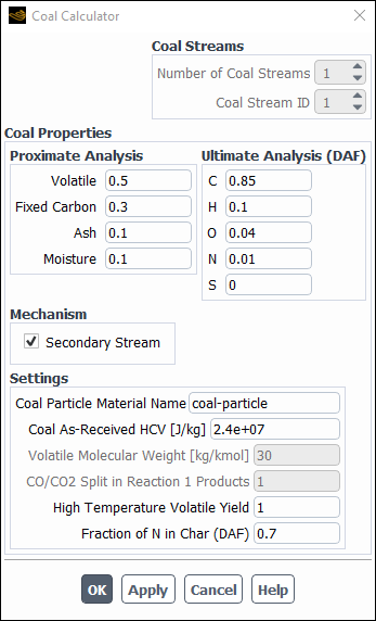
The inputs to the Coal Calculator dialog box are:
Coal Proximate Analysis, which is the mass fraction of Volatile, Fixed Carbon, Ash and Moisture in the coal.
Coal Ultimate Analysis, which is the mass fraction of atomic C, H, O, N and optionally S, in the Dry-Ash-Free (DAF) coal.
The option to use a Secondary Stream. If enabled, the two mixture fraction model will be set with the primary stream representing char as
 , and an empirical
secondary stream representing the volatiles.
, and an empirical
secondary stream representing the volatiles.The Coal Particle Material Name. A DPM Combusting Particle Material will be created with this name. The default name is coal-particle.
The Coal As-Received HCV (Higher Calorific Value).
The High Temperature Volatile Yield. Proximate analyses are generally done with slower heating rates and lower temperatures than would occur in a real flame. Therefore, enhanced devolatization at higher temperatures can cause the volatile yield to exceed the proximate analysis fraction. To model this, the actual volatile fraction used is calculated as that specified in the Proximate Analysis input multiplied by the High Temperature Volatile Yield. The actual Fixed Carbon fraction is then calculated as one minus the sum of the actual Volatile, Ash, and Moisture fractions.
Fraction of N in Char (DAF). This input is used in calculating the split of atomic nitrogen for the Fuel NOx model.
When the button is clicked, Ansys Fluent makes the following changes:
The empirical fuel atomic compositions in the Boundary tab are set, and the Non-Adiabatic model is enabled as required for DPM. The Empirical Fuel Lower Calorific Value is calculated as follows. First the DAF LCV of the coal is computed as,

(20–4)
where
 and
and  are the proximate moisture and ash fractions,
  is
the ultimate
is
the ultimate  fraction,
  and
and  are the molecular
weight of water and atomic hydrogen, respectively, and
are the molecular
weight of water and atomic hydrogen, respectively, and  is the latent heat of water.
If you are using the Secondary Stream option,
 is
calculated from
is
calculated from  using,
(20–5)
where
 and
and  are the proximate fixed carbon and volatile fractions, respectively.
A combusting particle material is created with Volatile Component Fraction and Combustible Fraction calculated from the ultimate and proximate analyses. The Discrete Phase Model (DPM) is enabled.
For the Fuel NOx model, the char N conversion is set to NO, and the Fuel NOx Volatile and Char mass fractions are set according to the ultimate and proximate compositions. Note that even though some of the Fuel NOx parameters are changed, the Fuel NOx model itself is not enabled.
After the Coal Calculator has set up the relevant models, you must build the PDF Table by clicking in the Table tab. You will also need to create injections if you have not done this yet. After converging your coal combustion case, you may want to enable the NOx model for postprocessing nitrogen-oxide pollutants.
For information about setting up control parameters, see the following sections:
Because Ansys Fluent calculates all intermediate and product species automatically during the equilibrium calculation, certain species will be included that are generally not in chemical equilibrium. Principal among these are the NOx species. Specifically, the NOx reaction rates are slow and should not be treated using an equilibrium assumption. Instead, the NOx concentration is predicted most accurately using the Ansys Fluent NOx postprocessor, where finite-rate kinetics are included (see NOx Formation). The NOx species can be safely excluded from the equilibrium calculation since they are present at low concentrations and have little impact on the density, temperature, and other species.
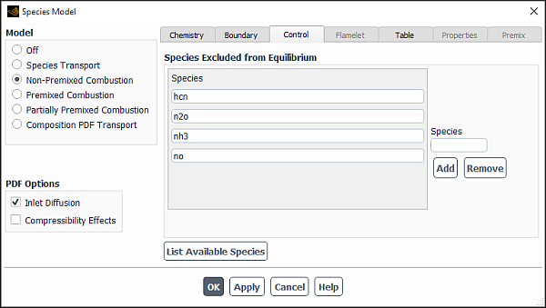
To force the exclusion of a species from the equilibrium calculation, click the Control tab in the Species Model dialog box (Figure 20.13: The Species Model Dialog Box (Control Tab)).
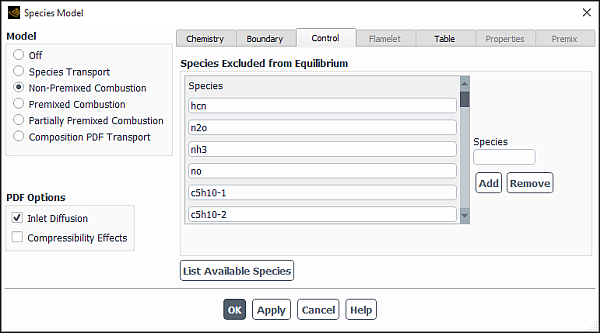
Under Species Excluded From Equilibrium, enter the chemical formula for the desired species in the Add/Remove Species field. Next, click to add the species to the Species list or Remove to remove an existing species from the Species list.
If there are species that you want to include in your PDF table that would be ignored by Ansys Fluent due to their low concentration (for example, CH, CH2, CH3 for the NOx calculation), you can force Ansys Fluent to include them using the text interface:
define → models → species → non-premixed-combustion
When the console window prompts you with Force Equilibrium
Species to Include..., specify
the appropriate species by entering the chemical formula(s) in double
quotes (for example, "ch", "ch2").
Note that you will have to first set up the inputs for the fuel and oxidizer before you are given the option to include the species.
When the steady diffusion flamelet model is selected, and you have created or imported a flamelet, you can adjust the controls for the flamelet solution in the Control tab of the Species Model dialog box (Figure 20.14: The Species Model Dialog Box (Control Tab) for the Steady Diffusion Flamelet Model).
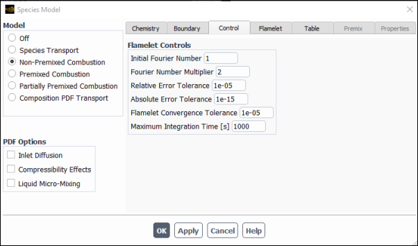
The Initial Fourier Number sets the first time step size for the solution of the flamelet equations (Equation 8–47 and Equation 8–48 in the Theory Guide). This first time step size is calculated as the explicit stability-limited diffusion time step size multiplied by this value. If the solution diverges before the first time step is complete, the value should be lowered.
The Fourier Number Multiplier increases the time step size at subsequent times. Every time step after the first is multiplied by this value. If the solution diverges after the first time step, this value should be reduced.
During the numerical integration of the flamelet equations, the local error is controlled to be less than
 | (20–6) |
where  represents the species
mass fractions and temperature at point
represents the species
mass fractions and temperature at point  in the 1D flamelet.
  is the value of the Relative
Error Tolerance and
is the value of the Relative
Error Tolerance and  is the value of the Absolute Error Tolerance, both of which you can specify.
Because steady flamelets are obtained by time-stepping, they are considered converged only when the maximum absolute change in species fraction or temperature at any discrete mixture-fraction point is less than the specified Flamelet Convergence Tolerance. Between time steps, the flamelet species fractions and temperature will sometimes oscillate, which causes absolute changes that are always greater than the flamelet convergence tolerance. In such cases, Ansys Fluent will stop the flamelet calculation after the total elapsed time has exceeded the Maximum Integration Time.
When modeling gas-phase combustion using the Eulerian unsteady laminar flamelet model, the flamelet fields are initialized to a burning, steady-flamelet solution in order to model ignition. However, assuming steady-flamelet profiles for slow-forming species is inaccurate. A better approximation is to identify the slow species and to set them to zero, which is done in the Control tab. By default, Ansys Fluent selects some NOx species (NO, NO2, N2O, N, NH, NH2, NH3, NNH, HCN, HNO, CN, H2CN, HCNN, HCNO, HOCN, HNCO, HCO), as well as liquid water H2<l> and solid carbon C<s> to be zeroed. See Figure 20.15: Method to Zero Out the Slow Chemistry Species.
For information about calculating flamelets, see the following sections:
In the Flamelet tab of the Species Model dialog box (Figure 20.16: The Species Model Dialog Box (Flamelet Tab)), you will enter values for parameters of the flamelet(s).
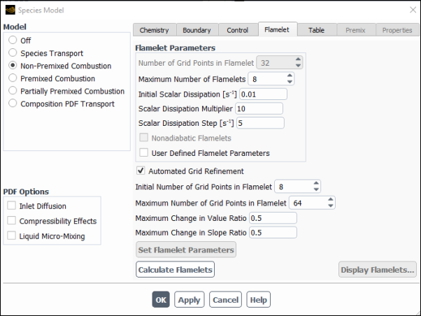
The Flamelet Parameters are as follows:
- Number of Grid Points in Flamelet
specifies the number of mixture fraction grid points distributed between the oxidizer (
 ) and the fuel (
 ). Increased resolution
will provide greater accuracy, but since the flamelet species and
temperature are solved coupled and implicit in
). Increased resolution
will provide greater accuracy, but since the flamelet species and
temperature are solved coupled and implicit in  space, the solution time and
memory requirements increase greatly with the number of
space, the solution time and
memory requirements increase greatly with the number of  grid points.
- Maximum Number of Flamelets
specifies the maximum number of flamelet profiles to be calculated. If the flamelet extinguishes before this number is reached, flamelet generation is halted and the actual number of flamelets in the flamelet library will be less than this value.
- Initial Scalar Dissipation
is the scalar dissipation of the first flamelet in the library. This corresponds to
 in Equation 8–53 in the Theory Guide.
- Scalar Dissipation Multiplier
specifies the ratio of the scalar dissipation step in which successive flamelets are generated when the scalar dissipation is less than 1 s-1. This corresponds to
 for
for  < 1 in Equation 8–53 in the Theory Guide.
- Scalar Dissipation Step
specifies the interval between scalar dissipation values (in s-1) for which multiple flamelets will be calculated. This corresponds to
 for
for  ≥ 1 in Equation 8–53 in the Theory Guide.
Note: Scalar Dissipation Multiplier and Scalar Dissipation Step are used to specify the interval of scalar dissipation for
 < 1 and
  ≥ 1, respectively. For example, for initial scalar dissipation of
1e-3 s-1 with a Scalar Dissipation
Multiplier of 10, and a Scalar Dissipation Step of 5, the
flamelets will be generated with scalar dissipations of 1e-3, 1e-2, 0.1, 1.0, 6, 11, 16, and
so on.
≥ 1, respectively. For example, for initial scalar dissipation of
1e-3 s-1 with a Scalar Dissipation
Multiplier of 10, and a Scalar Dissipation Step of 5, the
flamelets will be generated with scalar dissipations of 1e-3, 1e-2, 0.1, 1.0, 6, 11, 16, and
so on.- User Defined Flamelet Parameters
enables you to hook a user-defined function for scalar dissipation and mean mixture fraction (or progress variable) grid discretization
- Automated Grid Refinement
employs an adaptive algorithm, which inserts grid points so that the change of values, as well as the change of slopes, between successive grid points is less than user-specified tolerances. For information about this option, refer to Steady Diffusion Flamelet Automated Grid Refinement in the Theory Guide. Once this option is enabled, you can specify the following parameters:
- Initial Number of Grid Points in Flamelet
calculates a steady solution on a coarse grid, with a default of
 . See Equation 8–54 in the Theory Guide.
- Maximum Number of Grid Points in Flamelet
has a default of
 .
.- Maximum Change in Value Ratio
has a default of
 and is
  in Equation 8–28 in the Theory Guide.
- Maximum Change in Slope Ratio
has a default of
 and is
  in Equation 8–29 in the Theory Guide.
Click to begin the diffusion flamelet calculation. Sample output for a flamelet calculation is shown below.
 Generating flamelet 1 at scalar dissipation  0.01 /s

Time (s)   Temp (K)   Residual
1.679e-05   2233.7   3.779e+00
5.038e-05   2233.0   7.734e-02
1.175e-04   2231.5   1.648e-01
2.519e-04   2228.6   3.652e-01
5.206e-04   2223.6   8.295e-01
1.058e-03   2215.7   2.100e+00
2.133e-03   2205.5   3.540e+00
4.282e-03   2197.0   4.607e+00
8.581e-03   2193.6   6.639e+00
1.718e-02   2193.1   4.905e+00
3.437e-02   2193.4   5.792e+00
6.877e-02   2194.3   4.659e+00
1.375e-01   2195.3   3.922e+00
2.751e-01   2192.2   3.181e+00
5.502e-01   2188.6   2.549e+00
1.100e+00   2184.8   1.639e+00
2.201e+00   2182.9   4.604e+00
4.402e+00   2186.8   1.307e+00
8.804e+00   2189.6   4.420e-01
1.761e+01   2190.0   8.581e-02
3.522e+01   2190.0   1.199e-02
7.043e+01   2190.0   1.735e-03
1.409e+02   2190.0   4.217e-04
2.817e+02   190.0    6.892e-05
5.635e+02   2190.0   6.777e-06

Flamelet successfully generated
In the Flamelet tab of the Species Model dialog box (Figure 20.17: The Flamelet Tab for the Unsteady Diffusion Flamelet Model), you will enter values for parameters of the flamelet.
The Unsteady Flamelet Parameters are as follows:
- Number of Grid Points in Flamelet
specifies the number of mixture fraction grid points distributed between the oxidizer (
 ) and the fuel (
 ). Increased resolution
will provide greater accuracy, but since the flamelet species and
temperature are solved coupled and implicit in
). Increased resolution
will provide greater accuracy, but since the flamelet species and
temperature are solved coupled and implicit in  space, the solution time and
memory requirements increase with the number of
space, the solution time and
memory requirements increase with the number of  grid points.
- Mixture Fraction Lower Limit for Initial Probability
is the mixture fraction above which the marker probability will be initialized to 1, and below which the marker probability will be initialized to 0. In general, it should be set greater than the stoichiometric mixture fraction.
- Maximum Scalar Dissipation
is where flamelets extinguish at large scalar dissipation (mixing) rates. To prevent excessive mixing in the flamelet, Ansys Fluent allows you to specify a Maximum Scalar Dissipation rate for the 1D flamelet equations. A reasonable value for this is the steady flamelet extinction scalar dissipation. The default value of 30/s is near the steady extinction scalar dissipation of a methane-air flame at standard temperature and pressure.
- Courant Number
is the number at which Ansys Fluent automatically selects the time step for the probability equation based on this convective Courant number.
- Number of Flamelets
is the number of unsteady laminar flamelets to be initiated in the simulation. The probability marker equation will be solved for each flamelet.
Click to initialize the unsteady flamelet and its probability marker equation. Ansys Fluent is now ready for postprocessing the 1D unsteady flamelet and the 2D/3D unsteady marker probability equation.
The flamelet tables may be written to a file for import into later sessions of Ansys Fluent. You may want to do this, for example, to change the number of discretization points in the PDF table, or to plot the flamelet profiles in Ansys Fluent. The flamelet tables should be saved before you create the PDF table:
![]() File → Write → Flamelet...
File → Write → Flamelet...
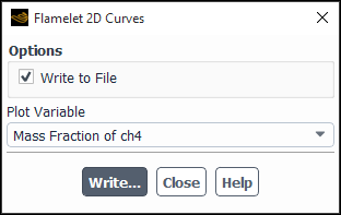
For the flamelet model, you can display or write flamelet curves. Click the or button. If you have a single flamelet, as for the unsteady diffusion flamelet model, you can access the Flamelet 2D Curves dialog box (Figure 20.18: The Flamelet 2D curves Dialog Box).
For the steady diffusion flamelet model with more than one flamelet, you can display 2D plots and 3D surfaces showing the variation of species fraction or temperature with the mean mixture fraction or scalar dissipation using the Flamelet 3D Surfaces dialog box (for example, Figure 20.19: The Flamelet 3D Surfaces Dialog Box).
To access this dialog box, click the button in the Flamelet tab of the Species Model dialog box, as shown in Figure 20.16: The Species Model Dialog Box (Flamelet Tab).
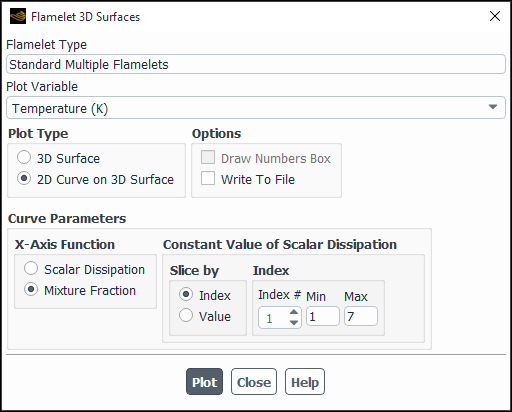
To display the flamelet tables graphically, use the following procedure:
In the Flamelet 3D Surfaces dialog box, from the Plot Variable drop-down list, select the variable you want to display graphically.
Specify the Plot Type as either 3D Surface or 2D Curve on 3D Surface.
For a 3D surface, enable or disable Draw Numbers Box under Options. When this option is turned on, the display will include a wireframe box with the numerical limits in each coordinate direction.
For a 2D curve on a 3D surface:
Specify whether you want to write the plot data to a file by toggling Write To File under Options.
Specify the X-Axis Function against which the plot variable will be displayed by selecting Scalar Dissipation (
 ), or Mixture Fraction (
 ). The variable that is not selected will be held
constant.
). The variable that is not selected will be held
constant.Specify the type of discretization (that is, how the flamelet data will be sliced) for the variable that is being held constant (under Constant Value of Mixture Fraction or Constant Value of Scalar Dissipation).
If you selected Index under Slice by, specify the discretization Index of the variable that is being held constant. The range of integer values that you are allowed to choose from is displayed under Min and Max, and is equivalent to the number of points specified for that variable in the Flamelet tab of the Species Model dialog box (see Calculating the Flamelets).
If you selected Value under Slice by, specify the numerical Value of the variable that is being held constant. The range of values that you can specify is displayed under Min and Max.
Write or display the flamelet table results. If you have turned on the Write To File option for a 2D plot, click and specify a name for the file in The Select File Dialog Box. Otherwise, click or as appropriate to display a 2D plot or 3D surface in the graphics window.
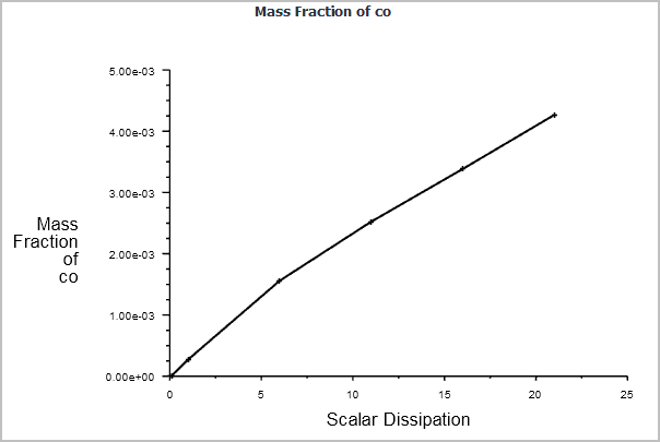
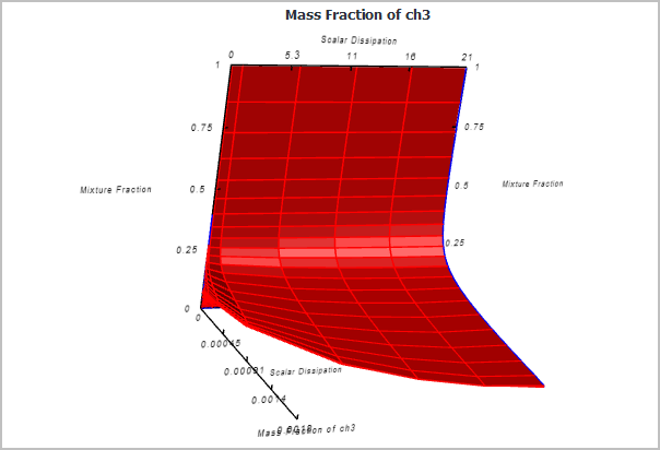
Figure 20.20: Example 2D Plot of Flamelet Data and Figure 20.21: Example 3D Plot of Flamelet Data show examples of a 2D curve plot and 3D surface plot of a flamelet table.
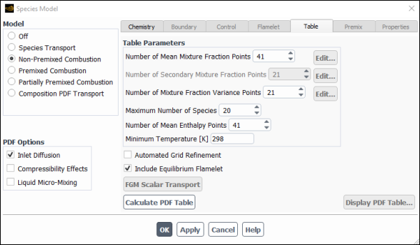
Ansys Fluent requires additional inputs that are used in the creation of the look-up tables. Several of these inputs control the number of discrete values for which the look-up tables will be computed. These parameters are input in the Table tab of the Species Model dialog box. When Automated Grid Refinement is enabled, you will specify the table parameters displayed in Figure 20.22: The Species Model Dialog Box (Table) Tab Displaying Automated Grid Refinement. If Automated Grid Refinement is disabled, you will specify the table parameters displayed in Figure 20.23: The Species Model Dialog Box (Table) Tab Excluding Automated Grid Refinement.
Note: Automated Grid Refinement is not available with two mixture fractions.
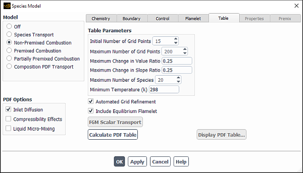
The look-up table parameters when Automated Grid Refinement is enabled are as follows:
- Initial Number of Grid Points
specifies the number of grid points for the resolution of the mean mixture fraction, mixture fraction variance, and mean enthalpy (for non-adiabatic systems).
- Maximum Number of Grid Points
specifies the maximum number of grid points used for tabulation. The grid refinement procedure will stop inserting the points when either the change in value and slope between successive points is within tolerance or the maximum number of grid points are generated.
- Maximum Change in Value Ratio
specifies the maximum allowable change in value of table variables between successive grid points as specified by Equation 8–28 in the Theory Guide.
- Maximum Change in Slope Ratio
specifies the maximum change in the slope of table variables between successive grid points as specified by Equation 8–29 in the Theory Guide.
- Maximum Number of Species
is the maximum number of species stored in the lookup tables.
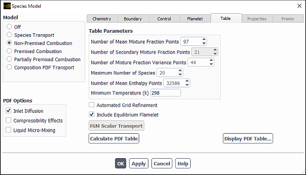
The look-up table parameters when Automated Grid Refinement is disabled are as follows:
- Number of Mean Mixture Fraction Points
is the number of discrete values of
 at which the look-up tables will
be computed. For a two-mixture-fraction model, this value is the number
of points in the instantaneous state profile used to compute the PDF
if you choose the
at which the look-up tables will
be computed. For a two-mixture-fraction model, this value is the number
of points in the instantaneous state profile used to compute the PDF
if you choose the  PDF model (see Tuning the PDF Parameters for Two-Mixture-Fraction Calculations). Increasing the number of points
will yield a more accurate PDF shape, but the calculation will take
longer. The mean mixture fraction points will be automatically clustered
around the stoichiometric mixture fraction value.
PDF model (see Tuning the PDF Parameters for Two-Mixture-Fraction Calculations). Increasing the number of points
will yield a more accurate PDF shape, but the calculation will take
longer. The mean mixture fraction points will be automatically clustered
around the stoichiometric mixture fraction value.- Number of Mixture Fraction Variance Points
is the number of discrete values of
 at which the look-up
tables will be computed. Lower resolution is acceptable because the
variation along the
at which the look-up
tables will be computed. Lower resolution is acceptable because the
variation along the  axis is, in general, slower than the variation
along the
axis is, in general, slower than the variation
along the  axis of the look-up tables. This option is available
only when no secondary stream has been defined.
axis of the look-up tables. This option is available
only when no secondary stream has been defined.- Number of Secondary Mixture Fraction Points
is the number of discrete values of
 at which the look-up tables will be computed. Like
the Number of Mean Mixture Fraction Points, Ansys Fluent will
use the Number of Secondary Mixture Fraction Points to compute the equilibrium state-relation if you choose the
at which the look-up tables will be computed. Like
the Number of Mean Mixture Fraction Points, Ansys Fluent will
use the Number of Secondary Mixture Fraction Points to compute the equilibrium state-relation if you choose the  PDF option (see Tuning the PDF Parameters for Two-Mixture-Fraction Calculations) for a two-mixture-fraction model.
A larger number of points will give a more accurate shape for the
PDF, but with a longer calculation time. This option is available
only when a secondary stream has been defined.
PDF option (see Tuning the PDF Parameters for Two-Mixture-Fraction Calculations) for a two-mixture-fraction model.
A larger number of points will give a more accurate shape for the
PDF, but with a longer calculation time. This option is available
only when a secondary stream has been defined.- Maximum Number of Species
is the maximum number of species that will be included in the look-up tables. The maximum number of species that can be included is 200. Ansys Fluent will automatically select the species with the largest mole fractions to include in the PDF table. Note that the PDF table values of density and specific heat are pre-calculated with all the species, and hence the convergence behavior of Ansys Fluent will not be affected by the input for the Maximum Number of Species. Hence, to keep table sizes small, you should set the Maximum Number of Species to only include the species that you are interested in postprocessing.
- Number of Mean Enthalpy Points
is the number of discrete values of enthalpy at which the look-up tables will be computed. This input is required only if you are modeling a non-adiabatic system. The number of points required will depend on the chemical system that you are considering, with more points required in high heat release systems (for example, hydrogen/oxygen flames). This option is not available with the unsteady flamelet model.
- Minimum Temperature
is used to determine the lowest temperature for which the look-up tables are generated. Your input should correspond to the minimum temperature expected in the domain (for example, an inlet or wall temperature). The minimum temperature should be set 10–20 K below the minimum system temperature. This option is available only if you are modeling a non-adiabatic system. This option is not available with the unsteady flamelet model.
- Include Equilibrium Flamelet
specifies that an equilibrium flamelet (that is,
 ) will be generated in Ansys Fluent and appended to the flamelet library before
the PDF table is calculated. This option is available when generating or importing multiple
flamelets, as well as when a single flamelet is considered. In the latter case, the PDF table
will consist of two scalar dissipation slices, namely the equilibrium slice at
) will be generated in Ansys Fluent and appended to the flamelet library before
the PDF table is calculated. This option is available when generating or importing multiple
flamelets, as well as when a single flamelet is considered. In the latter case, the PDF table
will consist of two scalar dissipation slices, namely the equilibrium slice at  , and the flamelet slice. This option is available only with the steady
diffusion flamelet model.
, and the flamelet slice. This option is available only with the steady
diffusion flamelet model.
When you are satisfied with your inputs, click to generate the look-up tables.
The computations performed for a single-mixture-fraction calculation culminate in the discrete integration of Equation 8–17 (or Equation 8–25 in the Theory Guide) as represented in Figure 8.5: Logical Dependence of Averaged Scalars on Mean Mixture Fraction, the Mixture Fraction Variance, and the Chemistry Model (Adiabatic, Single-Mixture-Fraction Systems) (or Figure 8.6: Logical Dependence of Averaged Scalars on Mean Mixture Fraction, the Mixture Fraction Variance, Mean Enthalpy, and the Chemistry Model (Non-Adiabatic, Single-Mixture-Fraction Systems) in the Theory Guide). For a two-mixture-fraction calculation, Ansys Fluent will calculate the physical properties using Equation 8–15 or its adiabatic equivalent. The computation time will be shortest for adiabatic single-mixture-fraction equilibrium calculations and longest for non-adiabatic calculations involving multiple flamelet generation. Below, sample outputs are shown for an adiabatic single-mixture-fraction equilibrium calculation and a non-adiabatic calculation with flamelets:
 Generating PDF lookup table
  Type of the PDF Table: Adiabatic Table (Two Streams)
 Calculating table .....

 1271 points calculated
 22 species added
 PDF Table successfully generated!
 Generating PDF lookup table
  Type of the PDF Table: Nonadiabatic Table with Strained Flamelet Model (Two Streams)
  Calculating table .....
  calculating temperature limits .....
  calculating temperature limits .....
  calculating scalar dissipation slices .....
   - scalar dissipation slice  9
  calculating equilibrium slice .....
 Performing PDF integrations.....

 16810 points calculated
 17 species added
 PDF Table successfully generated!
Initializing PDF table arrays and structures.
Important: Note that there is a significant difference in run time between the one-mixture fraction model and the two-mixture fraction model. In the one-mixture fraction model, the PDF table contains the mean data of density, temperature, and specific heats, and is three-dimensional for an equilibrium nonadiabatic case (mean mixture fraction, mixture fraction variance, and mean heat loss). For this case, Ansys Fluent updates properties every flow iteration. In the case of the two-mixture fraction model, only the instantaneous state relationships are stored and mean properties are calculated from these by performing PDF integrations in every cell of the Ansys Fluent simulation. Since this is computationally expensive, Ansys Fluent provides the option of only updating properties after a specified number of iterations.
For a two-mixture fraction model, you can also refer to Full Tabulation of the Two-Mixture-Fraction Model for more information.
After completing the calculation at the specified number of mixture fraction points, Ansys Fluent reports that the calculation succeeded. In a single-mixture-fraction case, the resulting look-up tables take the form illustrated in Figure 8.8: Visual Representation of a Look-Up Table for the Scalar (Mean Value of Mass Fractions, Density, or Temperature) as a Function of Mean Mixture Fraction and Mixture Fraction Variance in Adiabatic Single-Mixture-Fraction Systems in the Theory Guide (or Figure 8.10: Visual Representation of a Look-Up Table for the Scalar as a Function of Mean Mixture Fraction and Mixture Fraction Variance and Normalized Heat Loss/Gain in Non-Adiabatic Single-Mixture-Fraction Systems, for non-adiabatic systems). These look-up tables can be plotted using the available graphics tools, as described in Postprocessing the Look-Up Table Data.
Note that in non-adiabatic calculations, the console window will report that the temperature limits and enthalpy slices have been calculated.
For a two-mixture-fraction case, the resulting look-up tables take the form illustrated in Figure 8.9: Visual Representation of a Look-Up Table for the Scalar φ_I as a Function of Fuel Mixture Fraction and Secondary Partial Fraction in Adiabatic Two-Mixture-Fraction Systems in the Theory Guide (or Figure 8.11: Visual Representation of a Look-Up Table for the Scalar φ_I as a Function of Fuel Mixture Fraction and Secondary Partial Fraction, and Normalized Heat Loss/Gain in Non-Adiabatic Two-Mixture-Fraction Systems, for non-adiabatic systems).
The default algorithm for the two-mixture-fraction model is to perform PDF integrations of the equilibrium state relationships at run time. Since these are multi-dimensional integrals, the default two-mixture-fraction model can be computationally demanding.
Alternatively, you may want to pre-compute these integrations and create 4D look-up tables for adiabatic simulations, or 5D tables for non-adiabatic simulations. Such high-dimensional tables are computationally expensive to build, and may require large memory and disk storage, but can offer substantial improvement in run time speed.
The option to create a fully-tabulated two-mixture-fraction table is available in cases with the two-mixture-fraction model enabled, via the text command:
define/models/species/full-tabulation?
If you are modeling pollutant formation, note that the full tabulation option is not compatible with the mixture-fraction option for PDF Mode in the Turbulence Interaction Mode tab settings. See Setting Turbulence Parameters for details on Turbulence Interaction options for pollutant modeling.
Complex chemistry and non-adiabatic effects may make the equilibrium calculation more time-consuming and difficult. In some instances the equilibrium calculation may even fail. You may be able to eliminate any difficulties that you encounter by trying the calculation as an adiabatic system. Adiabatic system calculations are generally quite straightforward and can provide valuable insight into the optimal inputs to the non-adiabatic calculation.
Additional stability issues may arise for solid or heavy liquid fuels that have been defined using the empirical fuel approach. You may find that, for rich fuel mixtures, the equilibrium calculation produces very low temperatures and eventually fails. This indicates that strong endothermic reactions are taking place and the mixture is not able to sustain them. In this situation, you may need to raise the heating value of the fuel until Ansys Fluent produces acceptable results. Provided that your fuel will be treated as a liquid or solid (coal) fuel, you can maintain the desired heating value in your Ansys Fluent simulation. This is accomplished by defining the difference between the desired and the adjusted heating values as latent heat (in the case of combusting solid fuel) or heat of pyrolysis (in the case of liquid fuel).
The look-up tables may be stored in a file that you can read back into later sessions of Ansys Fluent. The look-up tables should be saved before you exit from the current Ansys Fluent session.
![]() File → Write → PDF...
File → Write → PDF...
By default, the file will be saved as formatted (ASCII, or text). To save a binary (unformatted) file, turn on the Write Binary Files option in the Select File dialog box.
It is important for you to view your temperature and species tables to ensure that they are adequately but not excessively resolved. Inadequate resolution will lead to inaccuracies, and excessive resolution will lead to unnecessarily slow calculation times.
After a PDF table has been generated or read into Ansys Fluent, you can display 2D plots and 3D surfaces showing the variation of species mole fraction, density, or temperature with the mean mixture fraction, mixture fraction variance, or enthalpy using the PDF Table dialog box (for example, Figure 20.24: The PDF Table Dialog Box (Non-Adiabatic Case With Flamelets)). The PDF Table dialog box can be accessed in one of two ways:
by clicking the button in the Table tab of the Species Model dialog box (as shown in Figure 20.23: The Species Model Dialog Box (Table) Tab Excluding Automated Grid Refinement)
by using the following path:
 Postprocessing
→ Model Specific → PDF Table...
Postprocessing
→ Model Specific → PDF Table...
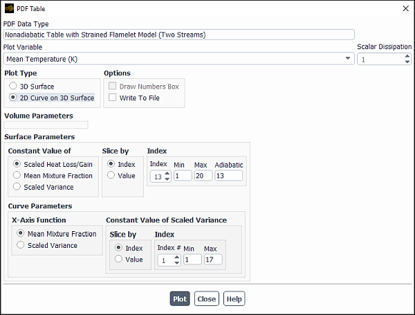
To display the look-up tables graphically, use the following procedure:
In the PDF Table dialog box, in the Plot Variable drop-down list you can select temperature, density, or species mole fraction as the variable to be plotted.
(multiple flamelets only) Specify the value of the Scalar Dissipation. In the case of non-adiabatic flamelets, there is the additional parameter of mean enthalpy. In addition to varying the mean enthalpy and mean mixture fraction, you can vary the display of the PDF table by changing the value of the scalar dissipation, which gives the table a fourth “dimension”.
Specify the Plot Type as either 3D Surface or 2D Curve on 3D Surface. In the equilibrium model, a 2D curve is a slice of a 3D surface, and therefore some options selected for a 3D surface may impact the display of a 2D curve.
For a 3D surface:
Enable or disable Draw Numbers Box under Options. When this option is turned on, the display will include a wireframe box with the numerical limits in each coordinate direction.
(non-adiabatic cases only) Under Surface Parameters, specify the discrete independent variable to be held constant in the look-up table (Constant Value of).
For a single-mixture-fraction case, select Scaled Heat Loss/Gain (
 ), Mean Mixture Fraction (
 ), or Scaled Variance (
 ). For any mean mixture fraction
  , the variance varies between a minimum of 0 and a maximum of
  . In order to view the mixture fraction variance, it is normalized by Equation 20–7 so that for any mean mixture fraction the scaled variance ranges from 0 to 0.25.
(20–7)
For a two-mixture-fraction case, the Scaled Heat Loss/Gain is the only available option.
(non-adiabatic cases only) Specify whether the 3D array of data points available in the look-up table will be sliced by Index or Value under Slice by.
If you selected Index, specify the discretization Index of the variable that is being held constant. The range of integer values that you are allowed to choose from is displayed under Min and Max, and is equivalent to the number of points specified for that variable in the Table tab of the Species Model dialog box (see Calculating the Look-Up Tables). If you specified to hold the enthalpy (Scaled Heat Loss/Gain) constant, the enthalpy slice index corresponding to the adiabatic case will be displayed in the Adiabatic field.
If you selected Value, specify the numerical Value of the variable that is being held constant. The range of values that you can specify is displayed under Min and Max.
For a 2D curve on a 3D surface:
Specify whether you want to write the plot data to a file by toggling Write To File under Options.
Under Curve Parameters, specify the X-Axis Function against which the plot variable will be displayed.
For an adiabatic single-mixture-fraction case, select Mean Mixture Fraction (
 ), or Scaled Variance (
 ).
).For a non-adiabatic single-mixture-fraction case, the options will depend on what was selected under Constant Value of under Surface Parameters, but will include two of the following: Scaled Heat Loss/Gain (
 ), Mean Mixture Fraction, and Scaled Variance.
For a two-mixture-fraction case, select Fuel Mixture Fraction (
 ) or Secondary Partial Fraction (
 ).
).
Specify the type of discretization (that is, how the look-up table data will be sliced) for the variable that is being held constant (under Constant Value of Mean Mixture Fraction, Constant Value of Scaled Variance, and so on). Note that for non-adiabatic cases, each 3D surface slice contains a full set of 2D slices.
If you selected Index under Slice by, specify the discretization Index of the variable that is being held constant. The range of integer values that you are allowed to choose from is displayed under Min and Max, and is equivalent to the number of points specified for that variable in the Table tab of the Species Model dialog box (see Calculating the Look-Up Tables).
If you selected Value under Slice by, specify the numerical Value of the variable that is being held constant. The range of values that you can specify is displayed under Min and Max.
Write or display the look-up table results. If you have turned on the Write To File option for a 2D plot, click and specify a name for the file in The Select File Dialog Box. Otherwise, click or as appropriate to display a 2D plot or 3D surface in the graphics window.
Figure 20.25: Mean Species Mole Fraction Derived From an Equilibrium Chemistry Calculation and Figure 20.26: Mean Temperature Derived From an Equilibrium Chemistry Calculation show examples of 2D plots derived for a very simple hydrocarbon system.
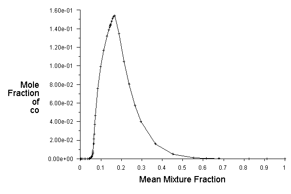
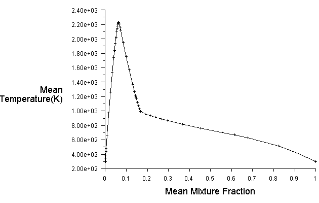
Figure 20.27: 3D Plot of Look-Up Table for Temperature Generated for a Simple Hydrocarbon System shows an example of a 3D surface derived for the same system.
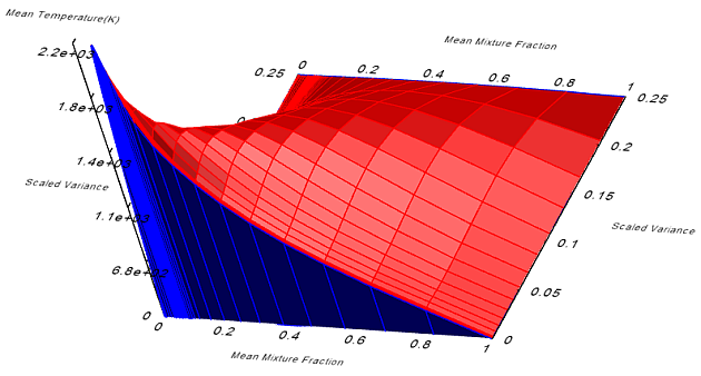
The standard flamelet file format can be used to read and write non-premixed (diffusion) flamelets. The data structure for the standard flamelet file format is based on keywords that precede each data section. If any of the keywords in your flamelet data file do not match the supported keywords, you will have to manually edit the file and change the keywords to one of the supported types. (The Ansys Fluent flamelet filter is case-insensitive, so you need not worry about capitalization within the keywords.)
The following keywords are supported by the Ansys Fluent filter:
|
Description |
Keyword |
|---|---|
|
Header section |
HEADER
|
|
Main body section |
BODY
|
|
Number of species |
NUMOFSPECIES
|
|
Number of grid points |
GRIDPOINTS
|
|
Pressure |
PRESSURE
|
|
Strain rate for diffusion flamelet generated in physical space |
STRAINRATE
|
|
Stoichiometric scalar dissipation for diffusion flamelet |
STOICH_SCADIS or CHI
|
|
Stoichiometric mixture fraction |
STOICH_Z
|
|
Temperature |
TEMPERATURE and TEMP
|
|
Mass fraction |
MASSFRACTION-
|
|
Mixture fraction |
Z
|
|
Mole fraction |
MOLEFRACTION-
|
Note: The strain rate output is written if the flamelets are generated in physical space, for example, using Ansys CHEMKIN.
A sample diffusion flamelet file in the standard format is provided below. Note that not all species are listed in this file.
 HEADER
 STOICH_SCADIS   1.000000E-02
 NUMOFSPECIES    60
 GRIDPOINTS      50
 STOICH_Z        6.618652E-02
 PRESSURE        1.013250E+05
 BODY
 Z
  0.000000000E+00 8.273315430E-03 1.240997314E-02 1.447830200E-02 1.551246643E-02
  1.602954865E-02 1.654663086E-02 2.068328857E-02 2.481994629E-02 3.309326172E-02
  4.136657715E-02 4.963989258E-02 5.377655029E-02 5.791320801E-02 6.204986572E-02
  6.618652344E-02 6.912528540E-02 7.206404735E-02 7.500280931E-02 7.794157127E-02
  7.867626176E-02 7.941095225E-02 8.088033323E-02 8.381909519E-02 8.675785714E-02
  8.969661910E-02 9.263538106E-02 9.557414302E-02 1.014516669E-01 1.073291909E-01
  1.132067148E-01 1.190842387E-01 1.249617626E-01 1.367168104E-01 1.425943343E-01
  1.484718583E-01 1.543493822E-01 1.572881441E-01 1.602269061E-01 1.672799348E-01
  1.743329635E-01 1.884390209E-01 2.166511357E-01 2.448632505E-01 2.730753653E-01
  3.407844408E-01 4.084935163E-01 5.709952975E-01 7.659974350E-01 1.000000000E+00
  TEMPERATURE
  3.000000000E+02 6.268546798E+02 7.802882604E+02 8.544333704E+02 8.908936814E+02
  9.089771589E+02 9.269654154E+02 1.067550740E+03 1.203418117E+03 1.462664100E+03
  1.707202552E+03 1.934669997E+03 2.037622483E+03 2.128475386E+03 2.200397351E+03
  2.244572249E+03 2.254177637E+03 2.245072250E+03 2.220638695E+03 2.186735136E+03
  2.177535664E+03 2.168109526E+03 2.148737393E+03 2.108856496E+03 2.068758176E+03
  2.029154219E+03 1.990673114E+03 1.953782923E+03 1.885112633E+03 1.821857119E+03
  1.761797286E+03 1.703540208E+03 1.647197627E+03 1.543457773E+03 1.496624533E+03
  1.452642813E+03 1.410968313E+03 1.390849359E+03 1.371237774E+03 1.326602075E+03
  1.286669965E+03 1.222176660E+03 1.134221753E+03 1.064763074E+03 1.004219101E+03
  8.845385948E+02 7.871510772E+02 6.152847269E+02 4.605312740E+02 3.000000000E+02
  massfraction-h
  0.000000000E+00 8.470246609E-15 1.689876963E-13 7.823505733E-13 1.604836416E-12
  2.259465253E-12 3.137901769E-12 2.297692554E-11 1.299314819E-10 2.009221085E-09
  3.364446760E-08 4.504321512E-07 1.488600091E-06 4.041919731E-06 9.259044043E-06
  1.764854561E-05 2.446982906E-05 2.948355957E-05 3.067005444E-05 2.858096141E-05
  2.763204904E-05 2.660609671E-05 2.447858861E-05 2.024662524E-05 1.571691024E-05
  1.207106883E-05 9.769042791E-06 8.144795604E-06 5.683704776E-06 3.862438419E-06
  2.529575950E-06 1.577642294E-06 9.493198194E-07 3.597224020E-07 2.397461608E-07
  1.672683885E-07 1.109095223E-07 8.352078253E-08 5.847760877E-08 2.024498078E-08
  6.804126487E-09 1.241975019E-09 1.664800458E-10 3.824650210E-11 1.058872219E-11
  1.103611172E-12 2.070333150E-13 5.521048377E-15 6.116361056E-17 0.000000000E+00
  massfraction-o2
  2.330000000E-01 2.037872969E-01 1.891809523E-01 1.818777426E-01 1.782261116E-01
  1.764002861E-01 1.745744526E-01 1.599674402E-01 1.453586904E-01 1.161277458E-01
  8.685446531E-02 5.764270922E-02 4.337649028E-02 2.986903537E-02 1.792882492E-02
  8.656537748E-03 4.260825775E-03 1.718417261E-03 5.787962652E-04 1.809733781E-04
  1.319197735E-04 9.626119601E-05 5.195145104E-05 1.624530279E-05 5.000207346E-06
  1.625791857E-06 5.935574928E-07 2.314963476E-07 5.242565474E-08 1.388575920E-08
  4.396692299E-09 1.701489188E-09 7.617025651E-10 3.172983452E-10 2.146818725E-10
  1.500353242E-10 1.052693603E-10 8.680804793E-11 7.032480088E-11 3.785587351E-11
  1.627110024E-11 1.631110236E-12 2.316226342E-14 1.904385354E-16 8.159316969E-19
  2.851864505E-21 7.569901388E-23 1.016058744E-25 1.304158252E-26 0.000000000E+00
  massfraction-oh
  .  .   .    .    .
  .  .   .    .    .
  .  .   .    .    .
Ansys Fluent will check whether all species in the flamelet data file exist in the thermodynamic properties databases thermo.db. If any of the species in the flamelet file do not exist, Ansys Fluent will issue an error message and halt the flamelet import. If this occurs, you can either add the missing species to the database, or remove the species from the flamelet file.
You should not remove a species from the flamelet data file unless its species concentration is very small (10-3 or less) throughout the flamelet profile. If you remove a low-concentration species, you will not have the species concentrations available for viewing in the Ansys Fluent calculation, but the accuracy of the Ansys Fluent calculation will otherwise be unaffected.
Important: If you choose to remove any species, be sure to also update the number of species (keyword NUMOFSPECIES) in the flamelet data file, to reflect the loss of any species you have removed from the file.
If a species with relatively large concentration is missing from the Ansys Fluent thermodynamic databases, you will have to add it. Removing a high-concentration species from the flamelet file is not recommended.
This section describes how to set up and apply the inert model. For a discussion about the theory, refer to Using the Non-Premixed Model with the Inert Model in the Theory Guide.
To enable the inert model, make sure that the non-premixed or partially premixed model is selected in the Species Model dialog box, or that a PDF file is read. Refer to Steps in Using the Non-Premixed Model and Modeling Partially Premixed Combustion to learn more about these models.
![]() Setup → Models →
Inert
Setup → Models →
Inert ![]() Edit...
Edit...
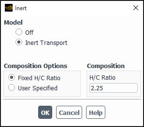
The Inert dialog box will be displayed (Figure 20.28: The Inert Model Dialog Box). To enable this model, select Inert Transport. The following steps will walk you through setting up the inert model:
Select Fixed H/C Ratio as the Composition Option if the hydrogen to carbon ratio is known. For example, for methane (CH4) enter
4for H/C Ratio.Setting the H/C ratio assumes that the burned gas resulted from the complete, stoichiometric combustion of that hydrocarbon fuel with air, and the only products of the combustion are CO2, H2O and N2.
Select User Specified as the Composition Option if you want to specify an arbitrary composition for the inert stream, as shown in Figure 20.29: The Inert Model Dialog Box.
You can specify your composition stream by adding or removing species if your stream is composed of species other than the default species list.
To add species to the Species list, type the chemical formula under Inert Species and click .
Enter the Mass Fraction of the newly added species. Continue in this manner until all of the inert species you want to include are shown in the Species list.
Make sure the sum of the mass fractions add up to 1. Ansys Fluent will normalize the species mass fractions for you when you click .
To remove a species from the list, type the chemical formula under Inert Species and click Remove.
To print a list of all species in the thermodynamic database file (
thermo.db) in the console window, click .
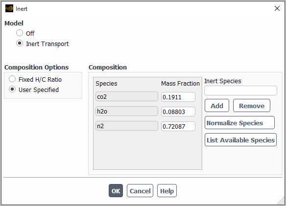
You will need to set appropriate boundary conditions at flow inlets and exits for the inert tracer mass fraction,  . The tracer species mass fraction must be between zero and one, with the value of one meaning that all of the material entering the domain comes from the inert stream. The values for flow boundaries are set in the Inert Stream field of the inlet boundary condition dialog boxes, under the Species tab.
The main assumption of the inert model is that the composition of the inert stream does not change with combustion. For some dilutants, this is a very reasonable assumption, however, it is not valid for rich combustion where there is fuel in the exhaust stream. For cases where there is fuel or oxidizer left in the exhaust gas, the accuracy of your results will depend upon taking the fuel or oxidizer species into account when setting initial conditions.
Initialization of the inert mass fraction  is done in the same way as other variables: by entering in the appropriate value in the Solution Initialization task page. Another option for initialization is to patch the value of
  in a region of the domain. When the value of
  is patched in this way, Ansys Fluent automatically recalculates the enthalpy field for the current temperature field in order to account for the change in composition.
See Patching Values in Selected Cells for details about patching values of solution variables.
For combustion calculations that burn a hydrocarbon fuel, Ansys Fluent provides a straightforward way of setting the initial composition of the inert stream. The inert composition can be set by assuming a ratio of hydrogen to carbon in the following overall oxidation reaction (from Heywood [63]):
 | (20–8) |
which can be rewritten in terms of the ratio of hydrogen to carbon atoms ( ) in the fuel as
 | (20–9) |
If Equation 20–9 is solved for the mass fractions of CO2, H2O and N2, the following relations are obtained:
 | (20–10) |
where

Setting the H/C ratio assumes that the burned gas resulted from the complete, stoichiometric combustion of that hydrocarbon fuel, and the only products of the combustion are CO2, H2O and N2. An arbitrary composition for the inert stream can also be specified in the interface.
Ansys Fluent allows burned gases to be converted to an inert gas. This has been designed with in-cylinder combustion in mind to aid the simulation of multiple cycles of such engines using the partially-premixed combustion model with exhaust gas recirculation (EGR). At the end of a combustion stroke, the premixed progress variable of the burnt gases is unity. When fresh charge, with progress variable of zero, is mixed with the burnt trapped gases, combustion will be initiated unless these trapped gases are converted to inert.
This facility is accessed via the Dynamic Mesh Events dialog box, as described in Resetting Inert EGR. There, you will need to set the crank angle at which the event occurs (usually shortly before the inlet valves open) and at the fluid zones (usually the combustion chamber) where the burnt gases are converted to inert.
When Ansys Fluent performs an inert reset, the inert composition is calculated as the stoichiometric composition. For lean mixtures, the stoichiometric inert is mixed with oxidizer, and for rich mixtures the stoichiometric inert is mixed with fuel, so that overall stoichiometry is conserved. This entails:
Calculating the stoichiometric mixture fraction, which is defined as the mixture where both fuel and oxidizer are completely consumed.
Calculating the inert species mass fractions as the stoichiometric species mass fractions. Species with mole fractions less than 0.01 are discarded.
Setting the inert mass fraction and the mixture fraction as follows:
Setting the reaction progress to zero.
For the G-Equation model, G (the mean distance from the flame front) is set to a negative value.
Since there will be some small errors in the species mass fractions from before the EGR reset, the temperature will change due to the change in the specific heat. By default, Ansys Fluent adjusts the enthalpy so that temperature is unchanged after EGR reset. This may be limited by the PDF table temperature limits for the new mixture fraction, in which case the temperature after inert reset will not equal the temperature before the inert reset event.


For information about defining non-premixed boundary conditions, see the following sections:
When the non-premixed combustion model is used, flow boundary
conditions at inlets and exits (that is, velocity or pressure, turbulence
intensity) are defined in the usual way. Species mass fractions at
inlets are not required. Instead, you define values for the mean mixture
fraction,  , and the mixture fraction variance,
  , at inlet boundaries.
(For problems that include a secondary stream, you will define boundary
conditions for the mean secondary partial fraction and its variance
as well as the mean fuel mixture fraction and its variance.) These
inputs provide boundary conditions for the conservation equations
you will solve for these quantities. The inlet values are supplied
in the boundary conditions task page, under the available tabs, for
the selected inlet boundary (for example, Figure 20.30: The Velocity Inlet Dialog Box Showing Mixture Fraction Boundary
Conditions).
, at inlet boundaries.
(For problems that include a secondary stream, you will define boundary
conditions for the mean secondary partial fraction and its variance
as well as the mean fuel mixture fraction and its variance.) These
inputs provide boundary conditions for the conservation equations
you will solve for these quantities. The inlet values are supplied
in the boundary conditions task page, under the available tabs, for
the selected inlet boundary (for example, Figure 20.30: The Velocity Inlet Dialog Box Showing Mixture Fraction Boundary
Conditions).
![]() Setup →
Setup → ![]() Boundary Conditions
Boundary Conditions
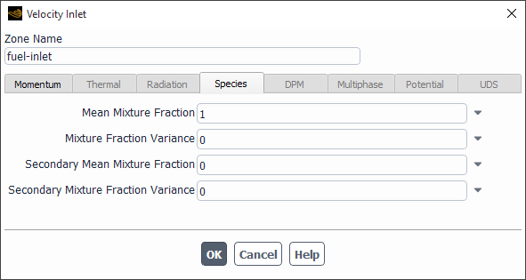
Click the Species tab and specify the Mean Mixture Fraction and Mixture Fraction Variance (and the Secondary Mean Mixture Fraction and Secondary Mixture Fraction Variance, if you are using two mixture fractions). In general, the inlet value of the mean fractions will be 1.0 or 0.0 at flow inlets: the mean fuel mixture fraction will be 1.0 at fuel stream inlets and 0.0 at oxidizer or secondary stream inlets; the mean secondary mixture fraction will be 1.0 at secondary stream inlets and 0.0 at fuel or oxidizer inlets. The fuel or secondary mixture fraction will lie between 0.0 and 1.0 only if you are modeling flue gas recycle, as illustrated in Figure 8.15: Using the Non-Premixed Model with Flue Gas Recycle and discussed in Definition of the Mixture Fraction in the Theory Guide. The fuel or secondary mixture fraction variance can usually be taken as zero at inlet boundaries.
In some cases, you may want to include the diffusive transport of mixture fraction through the inlets of your domain. You can do this by enabling inlet mixture-fraction diffusion. By default, Ansys Fluent excludes the diffusion flux of mixture fraction at inlets. To enable inlet diffusion, use either the
define/models/ species/inlet-diffusion?
text command, or the Species Model dialog box (Figure 20.1: Defining Equilibrium Chemistry)
![]() Setup → Models → Species
Setup → Models → Species ![]() Edit...
Edit...
and enable the Inlet Diffusion option.
If your model is non-adiabatic, you should specify the Temperature at the flow inlets. Recall that the inlet temperatures were requested during the table construction in the Chemistry tab of the Species Model dialog box, and were used in the construction of the look-up tables. The inlet temperatures for each fuel, oxidizer, and secondary inlet in your non-adiabatic model should be defined, in addition, as boundary conditions in Ansys Fluent. It is acceptable for the inlet temperature boundary conditions to differ slightly from those you input for the look-up table calculations. If the inlet temperatures differ significantly from those in the Chemistry tab, however, your look-up tables may provide inaccurate interpolation. This is because the discrete points in the look-up tables were clustered around a finite range of the temperatures defined in the Chemistry tab, and your input in the Ansys Fluent inlet boundary condition may fall outside this range.
Wall thermal boundary conditions should also be defined for non-adiabatic non-premixed combustion calculations. You can use any of the standard conditions available in Ansys Fluent, including specified wall temperature, heat flux, external heat transfer coefficient, or external radiation. If radiation is to be included within the domain, the wall emissivity should be defined as well. See Thermal Boundary Conditions at Walls for details about thermal boundary conditions at walls.
When you use the non-premixed combustion model, the material used for all fluid zones is automatically set to pdf-mixture. This material is a special case of the mixture material concept discussed in Mixture Materials. The constituent species of this mixture are the species that were calculated in the PDF look-up table creation; you cannot change them directly. When the non-premixed model is used, heat capacities, molecular weights, and enthalpies of formation for each species considered are extracted from the chemical database, so you will not modify any properties for the constituent species in the PDF mixture. For the PDF mixture itself, the mean density and mean specific heat are determined from the look-up tables.
The physical property inputs for a non-premixed combustion problem are therefore only the transport properties (viscosity, thermal conductivity, and so on) for the PDF mixture. To set these in the Create/Edit Materials Dialog Box, choose mixture as the Material Type, pdf-mixture (the default, and only choice) in the Mixture Materials list, and set the desired values for the transport properties.
![]() Setup →
Setup → ![]() Materials
Materials
See Physical Properties for details about setting physical properties. The transport properties in a non-premixed combustion problem can be defined as functions of temperature, if desired, but not as functions of composition. In practice, since turbulence effects will dominate, it will be of little benefit to include even the temperature dependence of the laminar transport properties.
If you are modeling radiation heat transfer, you will also enter radiation properties, as described in Radiation Properties. Composition-dependent absorption coefficients (using the WSGGM) are allowed.
The non-premixed model can also be used with real gas models in Ansys Fluent, if the Compressibility Effects option is enabled in the Species Model dialog box. In this case, the density method is based on one of the four real gas models, discussed in Equation of State and Using the Cubic Equation of State Real Gas Models.
The non-premixed model setup and solution procedure in Ansys Fluent differs slightly for single- and two-mixture-fraction problems. Below, an overview of each approach is provided. Note that your Ansys Fluent case file must always meet the restrictions listed for the non-premixed modeling approach in Restrictions on the Mixture Fraction Approach in the Theory Guide. In this section, details are provided regarding the problem definition and calculation procedures you follow in Ansys Fluent.
For additional information, see the following sections:
For a single-mixture-fraction system, when you have completed
the calculation of the PDF look-up tables, you are ready to begin
your reacting flow simulation. In Ansys Fluent, you will solve the flow
field and predict the spatial distribution of  and
and  (and
(and  if the system is non-adiabatic or
  if the system is based on laminar
flamelets). Ansys Fluent will obtain the corresponding values of temperature
and individual chemical species mass fractions from the look-up tables.
if the system is based on laminar
flamelets). Ansys Fluent will obtain the corresponding values of temperature
and individual chemical species mass fractions from the look-up tables.
When a secondary stream is included, Ansys Fluent will solve
transport equations for the mean secondary partial fraction ( ) and its variance in addition to the mean fuel mixture
fraction and its variance. Ansys Fluent will then look up the instantaneous
values for temperature, density, and individual chemical species in
the look-up tables, compute the PDFs for the fuel and secondary streams,
and calculate the mean values for temperature, density, and species.
) and its variance in addition to the mean fuel mixture
fraction and its variance. Ansys Fluent will then look up the instantaneous
values for temperature, density, and individual chemical species in
the look-up tables, compute the PDFs for the fuel and secondary streams,
and calculate the mean values for temperature, density, and species.
Note that in order to avoid both inaccuracies and unnecessarily slow calculation times, it is important for you to view your temperature and species tables in Ansys Fluent to ensure that they are adequately but not excessively resolved.
You can read a previously defined Ansys Fluent case file as a starting point for your non-premixed combustion modeling. If this case file contains inputs that are incompatible with the current non-premixed combustion model, Ansys Fluent will alert you when the non-premixed model is turned on and it will turn off those incompatible models. For example, if the case file includes species that differ from those included in the PDF file created by Ansys Fluent, these species will be disabled. If the case file contains property descriptions that conflict with the property data in the chemical database, these property inputs will be ignored.
Important: PDF files created by prePDF 2 or older are not supported by this version of Ansys Fluent. The files generated by PrePDF version 3 or newer, are fully compatible.
In the Species Model dialog box, select Non-Premixed Combustion under the Model heading. When you click in the Species Model dialog box, The Select File Dialog Box will immediately appear, prompting you for the name of the PDF file containing the look-up tables created in a previous Ansys Fluent session. (The PDF file is the file you saved using the File/Write/PDF... ribbon tab item after computing the look-up tables.) Ansys Fluent will indicate that it has successfully read the specified PDF file:
 Reading "/home/mydirectory/adiabatic.pdf"...
 read 5 species (binary c, adiabatic fluent)
 pdf file successfully read.
 Done.
After you read in the PDF file, Ansys Fluent will inform you that some material properties have changed. You can accept this information; you will be updating properties later on.
You can read in an altered PDF file at any time by using the File/Read/PDF... ribbon tab item.
Important: Recall that the non-premixed combustion model is available only when you used the pressure-based solver; it cannot be used with the density-based solvers. Also, the non-premixed combustion model is available only when turbulence modeling is active.
If you are modeling a non-adiabatic system and you want to include the effects of compressibility, re-open the Species Model dialog box and turn on Compressibility Effects under PDF Options. This option tells Ansys Fluent to update the density according to Equation 20–1. When the non-premixed combustion model is active, you can enable compressibility effects only in the Species Model dialog box. For other models, you will specify compressible flow (ideal-gas, boussinesq, and so on) in the Create/Edit Materials dialog box. See Specifying the Operating Pressure for the System and Tuning the PDF Parameters for Two-Mixture-Fraction Calculations for more information about compressibility effects.
The PDF filename is specified to Ansys Fluent only once. Thereafter, the filename is stored in your Ansys Fluent case file and the PDF file will be automatically read into Ansys Fluent whenever the case file is read. Ansys Fluent will remind you that it is reading the PDF file after it finishes reading the rest of the case file by reporting its progress in the text (console) window.
Note that the PDF filename stored in your case file may not contain the full name of the directory in which the PDF file exists. The full directory name will be stored in the case file only if you initially read the PDF file through the GUI (or if you typed in the directory name along with the filename when using the text interface). In the event that the full directory name is absent, the automatic reading of the PDF file may fail (since Ansys Fluent does not know which directory to look in for the file), and you will need to manually specify the PDF file. The safest approaches are to use the GUI when you first read the PDF file or to supply the full directory name when using the text interface.
The next step in the non-premixed combustion modeling process in Ansys Fluent is the solution of the mixture fraction and flow equations. First, initialize the flow. By default, the mixture fraction and its variance have initial values of zero, which is the recommended value; you should generally not set nonzero initial values for these variables. See Initializing the Solution for details about solution initialization.
![]() Solution →
Solution → ![]() Initialization
Initialization
Next, begin calculations in the usual manner.
![]() Solution →
Solution → ![]() Run Calculation
Run Calculation
During the calculation process, Ansys Fluent reports residuals for
the mixture fraction and its variance in the fmean and fvar columns of the residual report:
iter       cont       x-vel       y-vel          k     epsilon       fmean       fvar
  28    1.57e-3     4.92e-4     4.80e-4    2.68e-2     2.59e-3     9.09e-1    1.17e+0
  29    1.42e-3     4.43e-4     4.23e-4    2.48e-2     2.30e-3     8.89e-1    1.15e+0
  30    1.28e-3     3.98e-4     3.75e-4    2.29e-2     2.04e-3     8.88e-1    1.14e+0
(For two-mixture-fraction calculations, columns for psec and pvar will also appear.)
The transport equations for the mean mixture fraction and mixture fraction variance are quite stable and high, under-relaxation can be used when solving them. By default, an under-relaxation factor of 1 is used for the mean mixture fraction (and secondary partial fraction) and 0.9 for the mixture fraction variance (and secondary partial fraction variance). If the residuals for these equations are increasing, you should consider decreasing these under-relaxation factors, as discussed in Setting Under-Relaxation Factors.
One of the main reasons a combustion calculation can have difficulty converging is that large changes in temperature cause large changes in density, which can, in turn, cause instabilities in the flow solution. Ansys Fluent allows you to under-relax the change in density to alleviate this difficulty. The default value for density under-relaxation is 1, but if you encounter convergence trouble you may want to reduce this to a value between 0.5 and 1 (in the Solution Controls task page).
Note that if you are using a real-gas model the solution might converge at a slower rate than when running ideal-gas flow. To improve the convergence performance of your analysis, you need to reduce the underrelaxation for density to values as low as 0.1.
For cases that include a secondary stream, the PDF integrations are performed inside Ansys Fluent.
The parameters for these integrations are defined in the Species Model Dialog Box (Figure 20.31: The Species Model Dialog Box for a Two-Mixture-Fraction Calculation).
![]() Setup → Models → Species
Setup → Models → Species ![]() Edit...
Edit...
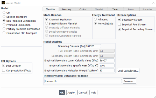
The parameters are as follows:
- Compressibility Effects
(non-adiabatic systems only) tells Ansys Fluent to update the density, temperature, species mass fraction, and enthalpy from the PDF tables to account for the varying pressure of the system.
You may be able to increase the robustness of combustion simulations that use a PDF table by
applying poor mesh numerics during the calculation. When you initialize or read data for a case
with non-premixed or partially premixed combustion, a cell register named
pdf_stability_marker is created (which marks cells where the
enthalpy—as defined by the PDF Table Heat Loss/Gain field variable
described in Alphabetical Listing of Field Variables and Their Definitions—is below the minimum PDF table value), and
this cell register is used as part of the settings for a register-based definition named
pmn_pdf_stability_marker that applies poor mesh numerics treatment every
5 iterations (for steady cases) or every 2 time steps (for unsteady cases). Note that this
definition is automatically created, but is deactivated by default; in order to use it in the
current session of Fluent, you must enter the following text command prior to running the
calculation:
> solve/set/poor-mesh-numerics/register-based/edit pmn_pdf_stability_marker active? yes
If you would like to use such definitions in all future sessions of Fluent without having to enter the previous text command, you can enable the Robust Numerics for Combustion with PDF Tables option in the Simulation branch of the Preferences dialog box (accessed through File/Preferences...).
Note that if the default settings for this treatment are not appropriate for your case, you can edit the cell register and/or register-based definition for poor mesh numerics, as described in Manage Cell Registers and Robustness with Meshes of Poor Quality, respectively.
The final step in the non-premixed combustion modeling process is the postprocessing of species concentrations and temperature data from the mixture fraction and flow-field solution data. The following variables are of particular interest:
Mean Mixture Fraction (in the Pdf... category)
Secondary Mean Mixture Fraction (in the Pdf... category)
Mixture Fraction Variance (in the Pdf... category)
Secondary Mixture Fraction Variance (in the Pdf... category)
Fvar Prod (in the Pdf... category, which is the production term in the mixture fraction variance transport equation)
Fvar2 Prod (in the Pdf... category)
Scalar Dissipation (in the Pdf... category)
PDF Table Adiabatic Enthalpy (in the Pdf... category)
PDF Table Heat Loss/Gain (in the Pdf... category)
Mass fraction of
species-n(in the Species... category)Mole fraction of
species-n(in the Species... category)Molar Concentration of
species-n(in the Species... category)RMS
species-nMass Fraction (in the Species... category)Static Temperature (in the Temperature... category)
RMS Temperature (in the Temperature... category)
Enthalpy (in the Temperature... category)
Probability (in the Unsteady Flamelet... category)
Mean Temperature (in the Unsteady Flamelet... category)
Mean Mass Fraction of
species-n(in the Unsteady Flamelet... category)
Important: For the unsteady diffusion flamelet model, mean species mass fractions are displayed for the first fifty species in the flamelet kinetic mechanism.
These quantities can be selected for display in the indicated category of the variable-selection drop-down list that appears in postprocessing dialog boxes. See Field Function Definitions for their definitions.
In all cases, the species concentrations are derived from the mixture fraction/variance field using the look-up tables. Note that temperature and enthalpy can be postprocessed even when your Ansys Fluent model is an adiabatic non-premixed combustion simulation in which you have not solved the energy equation. In both the adiabatic and non-adiabatic cases, the temperature is derived from the look-up table.
Figure 20.32: Predicted Contours of Mixture Fraction in a Methane Diffusion Flame and Figure 20.33: Predicted Contours of CO2 Mass Fraction Using the Non-Premixed Combustion Model illustrate typical results for a methane diffusion flame modeled using the non-premixed approach.
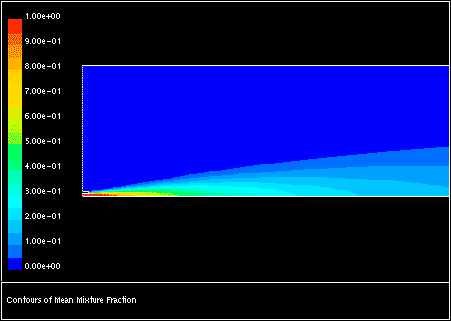
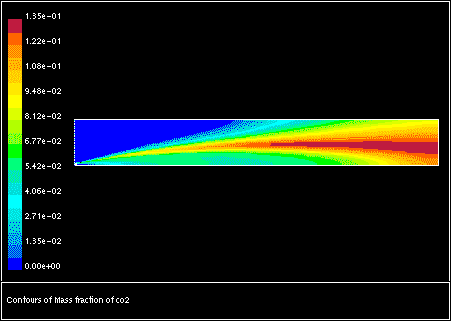
For additional information, see the following section:
Ansys Fluent provides several additional reporting options for post-processing calculations with the inert model. You can generate graphical plots or alphanumeric reports of the same items that are available with the non-premixed or partially premixed models, and in addition the following variables are available:
Inert Mass Fraction
Inert Specific Heat
Inert Density
Inert Enthalpy
Pdf Enthalpy
Pdf Fmean
Pdf Fvar
Mass Fraction of Inert

where the mass fraction of the  th inert
species,
th inert
species,  , is calculated as

where  is the inert tracer and
  is the mass fraction of the
  th inert
species defined in the Inert dialog box.
th inert
species defined in the Inert dialog box.
Note these variables appear in the Inert... category.