


This sections discusses how to simulate premixed turbulent combustion in Ansys Fluent. For theoretical background on this model, see Premixed Combustion in the Theory Guide.
Information about using this model is provided in the following sections:
The following limitations apply to the premixed combustion model:
You must use the pressure-based solver. The premixed combustion model is not available with the density-based solver.
The premixed combustion model is valid only for turbulent, subsonic flows. These types of flames are called deflagrations. Explosions, also called detonations, where the combustible mixture is ignited by the heat behind a shock wave, can be modeled with the finite-rate model using the density-based solver. See Modeling Species Transport and Finite-Rate Chemistry for information about the finite-rate model.
The premixed combustion model cannot be used in conjunction with the pollutant (that is, soot and NOx) models. However, a perfectly premixed system can be modeled with the partially premixed model (see Modeling Partially Premixed Combustion), which can be used with the pollutant models.
You cannot use the premixed combustion model to simulate reacting discrete-phase particles, because these would result in a partially premixed system. Only inert particles can be used with the premixed combustion model.
The G-Equation model can be used only with the unsteady solver because it tracks the flame front in time. However, RANS solutions, which tend to a steady-state, can be modeled by evolving them in time until the solution is stationary.
The procedure for setting up and solving a premixed combustion model is outlined below, and then described in detail. Remember that only the steps that are pertinent to premixed combustion modeling are shown here. For information about inputs related to other models that you are using in conjunction with the premixed combustion model, see the appropriate sections for those models.
Enable the premixed turbulent combustion model and set the related parameters.
Note: Make sure a turbulence model (other than the Spalart-Allmaras model) is selected before selecting a combustion model.
 Setup → Models → Species
  Edit...
Define the physical properties for the unburnt and burnt material in the domain.
Setup →  Materials → Create/Edit...
Set the value of the progress variable
 at flow inlets and exits. Setup → Boundary Conditions
 Initialize and patch the value of the progress variable.
Solution →
Initialization →  Patch...
Solve the problem and perform postprocessing.
Important: If you are interested in computing the concentrations of individual species in the domain, you can use the partially premixed model described in Modeling Partially Premixed Combustion. Alternatively, compositions of the unburnt and burnt mixtures can be obtained from external analyses using equilibrium or kinetic calculations.
For additional information, see the following sections:
To enable the premixed combustion model, select Premixed Combustion under Model in the Species Model Dialog Box (Figure 20.34: The Species Model Dialog Box for Premixed Combustion).
![]() Setup → Models → Species
Setup → Models → Species ![]() Edit...
Edit...
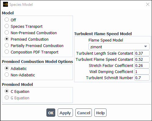
When you enable Premixed Combustion, the dialog box expands to show the relevant inputs.
Under Premixed Combustion Model Options in the Species Model Dialog Box, choose either Adiabatic (the default) or Non-Adiabatic. This choice affects only the calculation method used to determine the temperature (either Equation 8–97 or Equation 8–98 in the Theory Guide).
When C Equation or G Equation is selected as the Premixed Model, you can then choose to use the zimont or peters Flame Speed Model (described in Turbulent Flame Speed Models). You can also modify a number of model constants, as described in Modifying the Constants for the Zimont Flame Speed Model and Modifying the Constants for the Peters Flame Speed Model.
For a non-adiabatic premixed combustion model, note that the value you specify for the Turbulent Schmidt Number will also be used as the Prandtl number for energy. (The Energy Prandtl Number will therefore not appear in the Viscous Model dialog box for non-adiabatic premixed combustion models.) These parameters control the level of diffusion for the progress variable and for energy. The progress variable is closely related to energy (because the flame progress results in heat release), so it is important that the transport equations use the same level of diffusion.
For additional information, see the following sections:
- 20.2.3.1. Modifying the Constants for the Zimont Flame Speed Model
- 20.2.3.2. Modifying the Constants for the Peters Flame Speed Model
- 20.2.3.3. Additional Options for the G-Equation Model
- 20.2.3.4. Defining Physical Properties for the Unburnt Mixture
- 20.2.3.5. Setting Boundary Conditions for the Progress Variable
- 20.2.3.6. Initializing the Progress Variable
In general, you will not need to modify the constants used in the equations presented in C-Equation Model Theory in the Theory Guide. The default values are suitable for a wide range of premixed flames.
You can set the Turbulent Length Scale Constant ( in Equation 8–79), Turbulent Flame
Speed Constant (
in Equation 8–79), Turbulent Flame
Speed Constant ( in Equation 8–77), the Stretch
Factor Coefficient (
in Equation 8–77), the Stretch
Factor Coefficient ( in Equation 8–85), the Turbulent
Schmidt Number (
in Equation 8–85), the Turbulent
Schmidt Number ( in Equation 8–70), and the Wall Damping
Coefficient (
in Equation 8–70), and the Wall Damping
Coefficient ( in Equation 8–88).
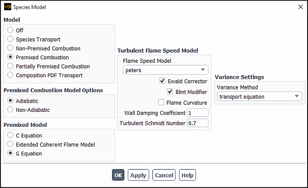
The Peters turbulent flame speed model constants, as described in Peters Flame Speed Model in the Theory Guide, are not available in the GUI because they are generally suitable for a wide range of premixed flames. They can, however, be accessed from the TUI.
The Ewald Corrector is enabled by default
and described in Peters Flame Speed Model. The Turbulent
Schmidt Number ( in Equation 8–70), and the Wall Damping
Coefficient (
in Equation 8–70), and the Wall Damping
Coefficient ( in Equation 8–88) are the same as those described for the Zimont model.
When the G-Equation model is enabled, the G Equation Settings group box appears. You can select either the transport equation or algebraic option for the calculation of the flame distance variance. Consult Peters Flame Speed Model in the Theory Guide for the variance transport and algebraic equation expressions (Equation 8–74 and Equation 8–75). It is recommended that you use the transport equation option for RANS and the algebraic option for LES.
When Flame Curvature Source is enabled, the curvature source term in the G-Equation, which is the last term in Equation 8–72, is included. By default, this term is excluded.
The fluid material in your domain should
be assigned the properties of the unburnt mixture, including the thermal
diffusivity ( in Equation 8–77 in the Theory Guide).
  is defined as
  , and values
at standard conditions can be found in combustion handbooks (for example, [83]).
, and values
at standard conditions can be found in combustion handbooks (for example, [83]).
For both adiabatic and non-adiabatic combustion models, you will need to specify the
Laminar Flame Speed ( in Equation 8–77 in the Theory Guide) as a material property, in the
Create/Edit Materials dialog box. You may choose to enter a
constant value, use a user-defined function, or apply
the metghalchi-keck-law. See Laminar Flame Speed in the Theory
Guide and Defining Physical Properties for the Unburnt Mixture for information about
setting the other properties for the unburnt material.
in Equation 8–77 in the Theory Guide) as a material property, in the
Create/Edit Materials dialog box. You may choose to enter a
constant value, use a user-defined function, or apply
the metghalchi-keck-law. See Laminar Flame Speed in the Theory
Guide and Defining Physical Properties for the Unburnt Mixture for information about
setting the other properties for the unburnt material.
When using the Zimont turbulent flame speed model, if you want
to include the flame stretch effect in your model, you will also need
to specify a lower value than the default Critical Rate
of Strain ( in Equation 8–86 in
the Theory Guide). As discussed in Flame Stretch Effect in the Theory Guide,
in Equation 8–86 in
the Theory Guide). As discussed in Flame Stretch Effect in the Theory Guide,  is set to a very high value (
 ) by default, so no flame stretching
occurs. To include flame stretching effects, you will need to adjust
the Critical Rate of Strain based on experimental
data for the burner. Because the flame stretching and flame extinction
can influence the turbulent flame speed (as discussed in Flame Stretch Effect in the Theory Guide), a realistic value for the Critical Rate of Strain is required for accurate predictions. Typical values for
) by default, so no flame stretching
occurs. To include flame stretching effects, you will need to adjust
the Critical Rate of Strain based on experimental
data for the burner. Because the flame stretching and flame extinction
can influence the turbulent flame speed (as discussed in Flame Stretch Effect in the Theory Guide), a realistic value for the Critical Rate of Strain is required for accurate predictions. Typical values for  lean premixed
combustion range from 3000 to 8000
lean premixed
combustion range from 3000 to 8000  [177]. Note that you can specify constant values or user-defined functions
to define the Laminar Flame Speed and Critical Rate of Strain. See the Fluent Customization Manual for details about user-defined functions.
[177]. Note that you can specify constant values or user-defined functions
to define the Laminar Flame Speed and Critical Rate of Strain. See the Fluent Customization Manual for details about user-defined functions.
For adiabatic models, you will also specify the Adiabatic
Burnt Temperature ( in Equation 8–97 in the Theory Guide), which
is the temperature of the burnt products under adiabatic conditions.
This temperature will be used to determine the linear variation of
temperature in an adiabatic premixed combustion calculation. You can
specify a constant value or use a user-defined function.
in Equation 8–97 in the Theory Guide), which
is the temperature of the burnt products under adiabatic conditions.
This temperature will be used to determine the linear variation of
temperature in an adiabatic premixed combustion calculation. You can
specify a constant value or use a user-defined function.
For non-adiabatic models, you will instead specify the Heat of Combustion per unit mass of fuel and the Unburnt Fuel Mass Fraction ( and
and  in Equation 8–99 in the Theory Guide). Ansys Fluent will
use these values to compute the heat losses or gains due to combustion,
and include these losses/gains in the energy equation that it uses
to calculate temperature. The Heat of Combustion can be specified only as a constant value, but you can specify a
constant value or use a user-defined function for the Unburnt
Fuel Mass Fraction.
in Equation 8–99 in the Theory Guide). Ansys Fluent will
use these values to compute the heat losses or gains due to combustion,
and include these losses/gains in the energy equation that it uses
to calculate temperature. The Heat of Combustion can be specified only as a constant value, but you can specify a
constant value or use a user-defined function for the Unburnt
Fuel Mass Fraction.
To specify the density for a premixed combustion model, choose premixed-combustion in the Density drop-down list and set the Adiabatic Unburnt Density and Adiabatic Unburnt Temperature ( and
and  in Equation 8–100 in
the Theory Guide). For adiabatic premixed models, your input for Adiabatic
Unburnt Temperature (
in Equation 8–100 in
the Theory Guide). For adiabatic premixed models, your input for Adiabatic
Unburnt Temperature ( ) will also be used in Equation 8–97 in the Theory Guide to
calculate the temperature.
) will also be used in Equation 8–97 in the Theory Guide to
calculate the temperature.
The other properties specified for the unburnt mixture are viscosity, specific heat, thermal conductivity, and any other properties related to other models that are being used in conjunction with the premixed combustion model.
For premixed combustion models, you will need to set an additional
boundary condition at flow inlets and exits: the progress variable,  . Valid inputs for the Progress Variable are as follows:
 : unburnt mixture
 : burnt mixture
Often, it is sufficient to initialize the progress variable  to 1 (burnt) everywhere
and allow the unburnt (
to 1 (burnt) everywhere
and allow the unburnt ( ) mixture entering the domain
from the inlets to blow the flame back to the stabilizer. A better
initialization is to patch an initial value of 0 (unburnt) upstream
of the flame holder and a value of 1 (burnt) in the downstream region
(after initializing the flow field in the Solution Initialization task page).
) mixture entering the domain
from the inlets to blow the flame back to the stabilizer. A better
initialization is to patch an initial value of 0 (unburnt) upstream
of the flame holder and a value of 1 (burnt) in the downstream region
(after initializing the flow field in the Solution Initialization task page).
![]() Solution →
Solution → ![]() Initialization → Patch...
Initialization → Patch...
See Patching Values in Selected Cells for details about patching values of solution variables.
Ansys Fluent provides several additional reporting options for premixed combustion calculations. You can generate graphical plots or alphanumeric reports of the following items:
Progress Variable
Damkohler Number
Stretch Factor
Turbulent Flame Speed
Static Temperature
Product Formation Rate
Laminar Flame Speed
Critical Strain Rate
Unburnt Fuel Mass Fraction
Adiabatic Flame Temperature
These variables are contained in the Premixed Combustion... category of the variable selection drop-down list that appears in postprocessing dialog boxes. See Field Function Definitions for a complete list of flow variables, field functions, and their definitions. Displaying Graphics and Reporting Alphanumeric Data explain how to generate graphics displays and reports of data.
Note that Static Temperature and Adiabatic Flame Temperature will appear in the Premixed Combustion... category only for adiabatic premixed combustion calculations; for non-adiabatic calculations, Static Temperature will appear in the Temperature... category. Unburnt Fuel Mass Fraction will appear only for non-adiabatic models.
Ansys Fluent also provides two additional reporting options for premixed combustion calculations with the G-Equation model:
Mean Distance from Flame
Variance of Distance from Flame
The Variance of Distance from Flame is the variance of the distance of the instantaneous flame from the mean flame position. These variables appear in the Premixed Combustion... category.
For additional information, see the following section:
If you know the composition of the unburnt and burnt mixtures in your model (that is, if you have performed separate Ansys Fluent or external analyses of chemical equilibrium calculations or 1D premixed flames), you can compute the species concentrations in the domain using custom field functions:
To determine the concentration of a species in the unburnt mixture, define the custom function
 , where
  is the mass fraction for the
species in the unburnt mixture (specified by you) and
is the mass fraction for the
species in the unburnt mixture (specified by you) and  is the value of the progress
variable (computed by Ansys Fluent).
is the value of the progress
variable (computed by Ansys Fluent).To determine the concentration of a species in the burnt mixture, define the custom function
 , where
  is the mass
fraction for the species in the burnt mixture (specified by you) and
is the mass
fraction for the species in the burnt mixture (specified by you) and  is the value of the progress
variable (computed by Ansys Fluent).
is the value of the progress
variable (computed by Ansys Fluent).
See Custom Field Functions for details about defining and using custom field functions.