For information about including viscous heating effects in your model, see Inclusion of the Viscous Dissipation Terms in the Theory Guide and Solving Heat Transfer Problems.

If you specify a nonzero gravity force (in the Operating Conditions Dialog Box), and you are modeling a non-isothermal flow, buoyancy effects can be included in the transport equations of the specified turbulence model as shown in Figure 15.31: SST Model with the Buoyancy Effects: Only Turbulence Production Option Enabled .

Figure 15.31: SST Model with the Buoyancy Effects: Only Turbulence Production Option Enabled

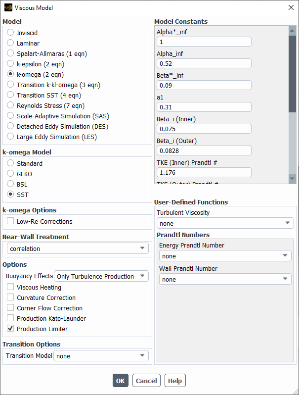
The following options are available:

Buoyancy effects can be included in the following turbulence models:

Eddy-viscosity models display an insensitivity to streamline curvature and system rotation, which play a significant role in many turbulent flows of practical interest, as described in Curvature Correction for the Spalart-Allmaras and Two-Equation Models in the Theory Guide. A modification to the turbulence production term is available to sensitize the following standard eddy-viscosity models to the effects of streamline curvature and system rotation:

Note that both the RNG and Realizable (-) turbulence models already have their own terms to include rotational or swirl effects (see RNG Swirl Modification and Modeling the Turbulent Viscosity in the Theory Guide for more information). The curvature correction option should therefore be used with caution for these two models and is offered mainly for completeness for RNG and Realizable (-).

Enable the Curvature Correction option under Options in the Viscous Model Dialog Box.

You can specify a value for CCURV under Curvature Correction Options to influence the strength of the curvature correction if needed for a specific flow. You have the option of specifying a constant, expression, or UDF.

Turbulent flows through rectangular channels, pipes of non-circular cross-section, and wing-body-junction type geometries exhibit secondary flows in the plane normal to the main flow direction into the corner along the bisector. To account for these secondary flows, you can enable Corner Flow Correction in the Options group box of the Viscous Model dialog box when you have selected one of the following turbulence models:

Figure 15.32: The Viscous Model Dialog Box with Corner Flow Correction option enabled

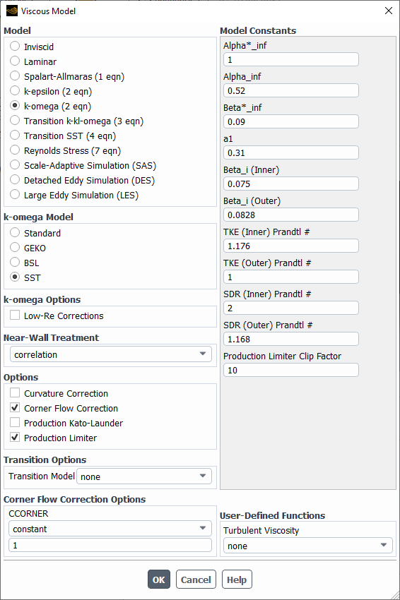
Afterwards, the Corner Flow Correction Options group box appears and you can set the coefficient CCORNER as a constant value, expression, or UDF.

For a detailed description of this option, see Corner Flow Correction in the Fluent Theory Guide.

For an example of specifying this option with a UDF, see DEFINE_CORNER_FLOW_CORRECTION_CCORNER in the Fluent Customization Manual.

The Compressibility Effects option is available under Options in the Viscous Model Dialog Box for most -based models, -based models, and Reynolds stress models when the compressible form of the ideal gas law or the real-gas model is enabled. This option can improve the prediction of free shear layers at high Mach numbers. See Model Enhancements for recommendations on when to use this option. For details about how this correction is implemented, see Effects of Compressibility on Turbulence in the k-ε Models and Compressibility Effects in the Theory Guide.

A disadvantage of standard two-equation turbulence models is the excessive generation of the turbulence energy, , in the vicinity of stagnation points. In order to avoid the buildup of turbulent kinetic energy in the stagnation regions, two formulations are available in order to limit the production term in the turbulence kinetic energy equations:

Both these formulations can be accessed under Options in the Viscous Model dialog box. The Production Limiter model coefficient is called the Production Limiter Clip Factor and has a default value of 10. This value can be modified under Model Constants once the Production Limiter formulation is enabled.

You can use the following text commands to set the formulations:

The Production Limiter is available for the following turbulence models:

By default, this limiter is enabled for all turbulence models based on the equation.

The Production Kato-Launder formulation for the production term is available for the following turbulence models:

The Kato-Launder formulation is enabled by default for the Transition SST model only.

For the Spalart-Allmaras model, you can choose either Vorticity-Based Production or Strain/Vorticity-Based Production under Spalart-Allmaras Production in the Viscous Model Dialog Box. If you choose Vorticity-Based Production, Ansys Fluent will compute the value of the deformation tensor using Equation 4–22 (in the Theory Guide); if you choose Strain/Vorticity-Based Production, it uses Equation 4–24 (in the Theory Guide).

(These options will not appear unless you have enabled the Spalart-Allmaras model.)

The Delayed DES option is recommended when using the DES model. This option preserves the RANS model throughout the boundary layer. For more information, see Detached Eddy Simulation (DES) in the Theory Guide.

The RNG turbulence model in Ansys Fluent has an option of using a differential formula for the effective viscosity (Equation 4–44 in the Theory Guide) to account for the low-Reynolds-number effects. To enable this option, the Differential Viscosity Model option under RNG Options in the Viscous Model Dialog Box must be enabled.

After you have chosen the RNG model, the swirl modification takes effect, by default, for all three-dimensional flows and axisymmetric flows with swirl. The default swirl constant ( in Equation 4–46 in the Theory Guide) is set to 0.07, which works well for weakly to moderately swirling flows. However, for strongly swirling flows, you may need to use a larger swirl constant.

To change the value of the swirl constant, you must first enable the Swirl Dominated Flow option under RNG Options in the Viscous Model Dialog Box.

If any of the - models or the Stress-Omega RSM is used, you may enable a low-Reynolds-number correction to the turbulent viscosity by enabling the Low-Re Corrections option under k-omega Options in the Viscous Model dialog box. By default, this option is not enabled, and the damping coefficient ( in Equation 4–75 in the Theory Guide) is equal to 1.

In the standard - model and the Stress-Omega RSM, you also have the option of including corrections to improve the accuracy in predicting free shear flows. The Shear Flow Corrections option under the k-omega Options is enabled by default in the Viscous Model dialog box, as these corrections are included in the standard - model  [173]. When this option is enabled, Ansys Fluent will calculate using Equation 4–85 (in the Theory Guide) and using Equation 4–92 (in the Theory Guide). If this option is disabled, and will be set equal to 1.

For cases that use the VOF or Mixture multiphase models, or the Eulerian multiphase model with the Multi-Fluid VOF option selected, you can enable Turbulence Damping (in the Turbulence Damping Options group box). This option is required for better resolution of velocity gradients in the vicinity of fluid-fluid interface. After enabling Turbulence Damping, you can specify the Damping Factor, which by default is set to 10. For a theoretical discussion about turbulence damping, refer to Turbulence Damping in the Fluent Theory Guide.

If the enhanced wall treatment is used, you may include the effects of pressure gradients by enabling the Pressure Gradient Effects option under the Enhanced Wall Treatment Options. When this option is enabled, Ansys Fluent will include the coefficient in Equation 4–372 (in the Theory Guide).

If the enhanced wall treatment is used, you may include thermal effects by enabling the Thermal Effects option under Enhanced Wall Treatment Options. When this option is enabled, Ansys Fluent will include the coefficient in Equation 4–372 (in the Theory Guide). will also be included in Equation 4–372 when the Thermal Effects option is enabled if the ideal gas law is selected for the fluid density in the Create/Edit Materials dialog box.

If the RSM is used with the default model for linear pressure-strain, Ansys Fluent will, by default, include the wall-reflection effects in the pressure-strain term. That is, Ansys Fluent will calculate using Equation 4–233 (in the Theory Guide) and include it in Equation 4–230 (in the Theory Guide). For the quadratic pressure-strain model, Stress-Omega model, and Stress-BSL model, the wall-reflection effects are not required and are not included.

For the -based Reynolds stress models, by default Ansys Fluent uses the explicit setting of boundary conditions for the Reynolds stresses near the walls, with the values computed with Equation 4–260 (in the Theory Guide). The turbulent kinetic energy, , is calculated by solving the equation obtained by summing Equation 4–226 (in the Theory Guide) for normal stresses. To disable this option and use the wall boundary conditions given in Equation 4–261 (in the Theory Guide), turn off the Wall BC from k Equation under the Reynolds-Stress Options in the Viscous Model dialog box.

To use the quadratic pressure-strain model described in Quadratic Pressure-Strain Model (in the Theory Guide), enable the Quadratic Pressure-Strain Model option under Reynolds-Stress Options in the Viscous Model Dialog Box. (This option will not appear unless you have enabled the RSM.) The following options are not available when the Quadratic Pressure-Strain Model is enabled:

To use the Stress-Omega model (described in Stress-Omega Model) or the Stress-BSL model (described in Stress-BSL Model), select Stress-Omega or Stress-BSL, respectively, from the Reynolds-Stress Model list in the Viscous Model Dialog Box. (These options will not appear unless you have enabled the RSM.) The following options are not available when the Stress-Omega or the Stress-BSL model is selected:

Instead, the following options are available:

If you have selected the Large Eddy Simulation model, you will be able to choose one of the subgrid-scale models described in Subgrid-Scale Models (in the Theory Guide). You can choose from the Smagorinsky-Lilly, WALE, WMLES, WMLES S-Omega, or Kinetic-Energy Transport subgrid-scale models. Note that Dynamic Stress is an option available with the Smagorinsky-Lilly model (and when it is enabled, this model is referred to as the “dynamic Smagorinsky” model), while the Kinetic-Energy Transport model is always run as a dynamic model. The Dynamic Fvar option is available for all of the subgrid-scale models when Non-Premixed Combustion or Partially Premixed Combustion is selected in the Species Model Dialog Box.

If you are using the Spalart-Allmaras, -, -, DES, or LES models, a UDF can be used to customize the turbulent viscosity. This option will enable you to modify in the case of the Spalart-Allmaras, -, and - models, and incorporate completely new subgrid models in the case of the LES model. SBES with BSL / SST allows the usage of a UDF in order to provide a custom formulation for in the RANS region, but not for the subgrid model in the LES region. More information about UDFs can be found in the Fluent Customization Manual.

In the Viscous Model Dialog Box, under User-Defined Functions, select the appropriate user-defined function in the Turbulent Viscosity drop-down list. For the LES model, select the appropriate UDF in the Subgrid-Scale Turbulent Viscosity drop-down list.

You can use UDFs to customize the turbulent Prandtl and Schmidt numbers. For the standard and realizable - models and the standard - model, your UDF can calculate the TKE Prandtl number () and either the TDR or SDR Prandtl number ( or ), depending on whether you are using the - or - model. All turbulence models allow you to use UDFs for the turbulent Prandtl number at the wall ( in Equation 4–343 in the Theory Guide), and all turbulent models except for the RNG - model allow you to use UDFs for the turbulent Prandtl number for energy ( in, for example, Equation 4–64 or Equation 4–251 in the Theory Guide), as well as the turbulent Schmidt number (, in Equation 7–4 in the Theory Guide) if species transport has been enabled. Note that UDFs cannot be used for the turbulent Prandtl number for energy or the turbulent Schmidt number if you have enabled Dynamic Energy Flux or Dynamic Scalar Flux, respectively, as part of the LES model. More information about UDFs can be found in the Fluent Customization Manual.

In the Viscous Model Dialog Box, under User-Defined Functions, select the appropriate UDF from the drop-down lists in the Prandtl Numbers or Prandtl and Schmidt Numbers group box. The options will depend on the turbulence model you have selected (as noted previously), and include: TKE Prandtl Number, TDR Prandtl Number, SDR Prandtl Number, Energy Prandtl Number, Wall Prandtl Number, and Turbulent Schmidt Number. Note that the availability of these drop-down lists can be affected by your settings for the energy equation and the multiphase and combustion models.

If the turbulent flow involves non-Newtonian fluids, you can use the define/models/ viscous/turbulence-expert/turb-non-newtonian? text command to enable the selection of non-Newtonian options for the material viscosity. See Viscosity for Non-Newtonian Fluids for details about these options.

You have the option of including Scale-Adaptive Simulation (SAS) with most -based URANS models. For details about SAS and how to include it, see Scale-Adaptive Simulation (SAS) and Setting Up Scale-Adaptive Simulation (SAS) Modeling, respectively.

You have the option of including Detached Eddy Simulation (DES) with the Transition SST model. For details about DES and how to include it, see Detached Eddy Simulation (DES) and Setting Up DES with the Transition SST Model, respectively.

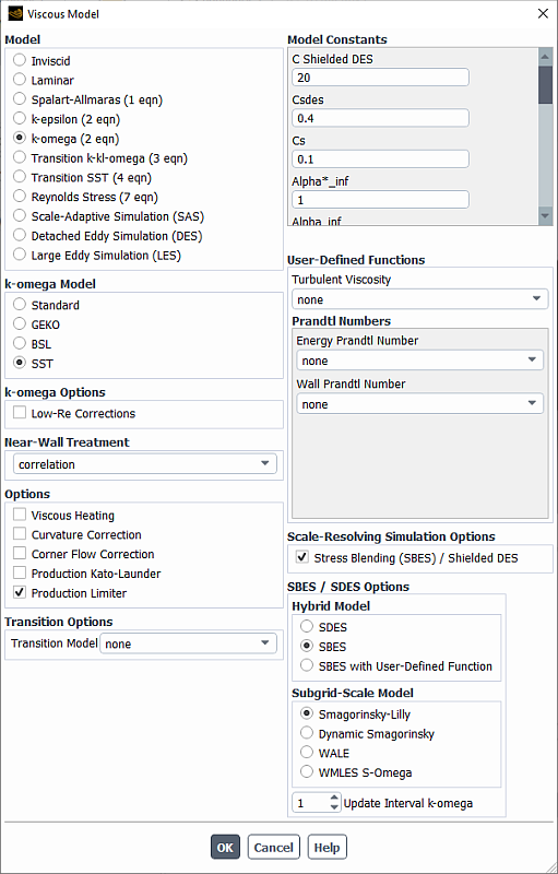
To enable a hybrid RANS-LES model with an improved shielding function compared to DDES / IDDES, you can enable the Stress Blending (SBES) / Shielded DES option in the Scale-Resolving Simulation Options group box of the Viscous Model dialog box. This option is available for 3D transient cases when you have selected one of the following models (see Figure 15.33: The Viscous Model Dialog Box with the SBES Options for -based RANS models):

You can then select one of the following from the Hybrid Model list:

If you select SBES or SBES with User-Defined Function for the Hybrid Model, you can also select one of the following subgrid-scale (LES) models:

The WALE model is recommended, as it provides the lowest eddy viscosity in 2D flow regions and thereby allows the flow to quickly develop 3D turbulence structures in separating shear layers. The combination of SBES with the WMLES S-Omega formulation is likely not a useful combination, as the SBES-WALE model combination can by itself act in a WMLES mode.

If you select SBES or SBES with User-Defined Function for the Hybrid Model, you can also specify an integer value (between 1 and 10) for Update Interval k-omega, which determines how often the and equations are computed during a run. This option is not available for the Realizable - model.

In many cases, the global time step size required for the LES portion of the calculation is unnecessarily small for the RANS portion. For this reason, it is not required that the - part of the SBES model is updated after every time step. Reducing the frequency at which the - equations are solved by specifying an update interval can positively impact the solution time, with minimal impact on the solution or convergence. An optimal value for the parameter is 5. Note that the momentum equations as well as the LES eddy-viscosity portion of the SBES model are updated at every time step. The parameter only reduces the number of updates of the and equations, as well as that of the blending function.

For example, if you specify an update interval of 5, the solver would update the - portion every 5th timestep, while still updating the LES eddy viscosity portion every timestep.

Figure 15.33: The Viscous Model Dialog Box with the SBES Options for -based RANS models

For the DES model with the BSL - model, SST - model, or the Transition SST model, the shielding (or blending) functions F1 and F2 are defined in Equation 4–108 and Equation 4–119 in the Theory Guide, respectively. Note that the F2 function is more conservative than the F1 function. In addition, the shielding functions DDES (Delayed DES) and IDDES (Improved Delayed DES), are described in DES with the BSL or SST k-ω Model and Improved Delayed Detached Eddy Simulation (IDDES) in the Theory Guide. DDES is recommended and is used as the default.