


The acoustics wave equation model is recommended to be used with scale-resolving simulations of turbulent flows at low Mach numbers (LES, SBES, DES, SAS). Due to the current limitation of constant density and sound speed in the background fluid flow, no significant variation of these two parameters due to non-uniform temperature or mixture composition is allowed.
It is highly recommended that you read Preventing Non-Physical Reflections of Sound Waves in the Fluent Theory Guide for strategies to improve simulation quality.
The wave equation model is available for transient flow simulations with the second order or bounded second order implicit time scheme active. The model is not available for the 2-D axisymmetric version of Fluent.
You can enable the Wave Equation using the TUI command:
/define/models/acoustics/wave-equation?
The wave equation options are found in the menu:
/define/models/acoustics/wave-equation-options
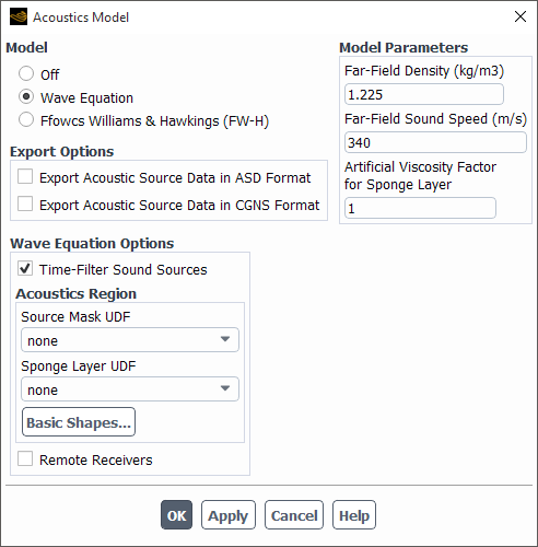
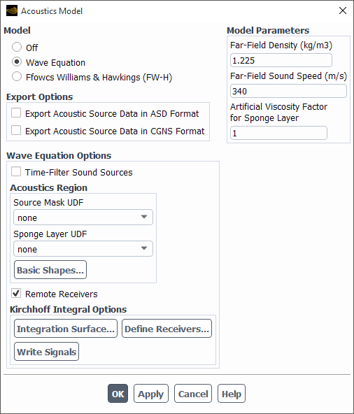
The field Artificial Viscosity Factor for Sponge Layer is used to
specify parameter C, which participates in Equation 11–13. The base
level of artificial viscosity  can be changed by the TUI command:
/define/models/acoustics/wave-equation-options/sponge-layer-base-level
The far-field parameters can be set using the TUI command:
/define/models/acoustics/far-field-parameters
The Acoustics Region group box is used to set up the geometry of the source mask and sponge regions.
There are two methods to define geometry data:
Preparing UDFs
Use of basic shapes (rectangular hexahedron, cylinder, sphere)
The two methods may be combined together. The source mask and the sponge layer UDFs are created using the following macros:
DEFINE_SOURCE_MASK(src_mask_define, c, t)
DEFINE_SPONGE_LAYER(sponge_define, c, t)
where src_mask_define and
sponge_define are example function names,
c is a cell number, and t is a pointer
to a cell thread. There can only be one UDF of each of these two types per simulation. Each
UDF returns a single real value, which fills a corresponding storage variable
(SV_SOUND_MODEL_SRC_MASK or
SV_SOUND_SPONGE) in the cell c of the
thread t.
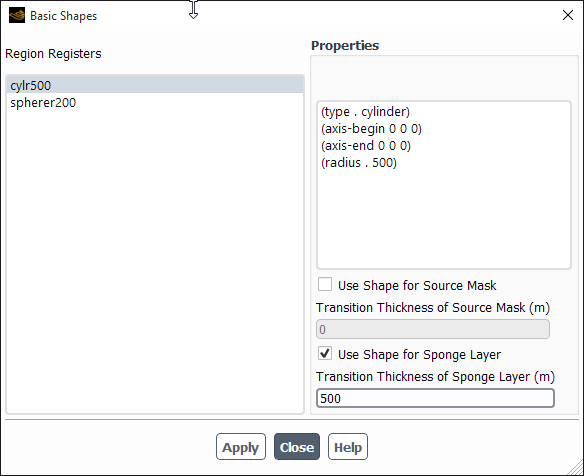
Simple geometries can be built out of the basic shapes (rectangular hexahedron, cylinder, sphere), which must be preliminarily defined as cell registers of the type Region.
![]() Solution → Cell Registers
Solution → Cell Registers
![]() New → Region...
New → Region...
After you create one or more cell registers, you can use them to specify the desired geometry by clicking Basic Shapes... in the Acoustics Model dialog box (Figure 23.16: The Acoustics Model Dialog Box), which opens the Basic Shapes dialog box (Figure 23.17: The Basic Shapes Dialog Box). In this window you can add cell registers to either the source mask or sponge layer geometry definitions, and specify the individual transition thickness for each shape for each purpose.
Note: After the cell registers have been used for the source mask and sponge layer geometry definitions, subsequent editing or deleting of these cell registers do not influence the already specified source mask and sponge layer geometry.
The TUI commands for creating and editing source mask and sponge layer geometry can be found in the menu:
/define/models/acoustics/wave-equation-options/basic-shapes/
To visualize the source mask and the sponge layer geometries, use the field variables
Sound WaveEq Model Source Mask and Sound Sponge Layer
Marker from the Acoustics… variable group. These
output fields directly show the storage variables
SV_SOUND_MODEL_SRC_MASK and
SV_SOUND_SPONGE without any transformations.
Note: The sponge layer described in this section is part of the wave equation model and is based on the viscosity. An alternative sponge layer model that is based on density is also available for compressible flows that use the pressure-based solver, as described in Sponge Layers.
When the wave equation model is active, the Solution Controls task page includes an additional frame titled Acoustics Wave Equation Solver Controls (see Figure 23.18: The Acoustics Wave Equation Solver Controls Task Page).
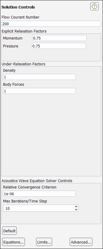
The parameters Relative Convergence Criterion and Max
Iterations/Time Step control the sub-iterations of the implicit wave equation
solver. The need for sub-iterations comes from explicit skewness corrections to the
discretization of the basic Laplacian term in Equation 11–11, as
well as the artificial viscosity term. At each sub-iteration, the system of linear equations
is processed by the AMG linear solver to reduce the residual norm by a factor of 0.1 (this
can be controlled by changing the rp-variable
acoustics-waveeq/amg-alpha). The optimal values of these three
algorithm parameters may depend on the mesh quality. Their default values may change in
future releases after accumulating more experience with the wave equation model.
The TUI commands for the acoustics wave equation solution controls are found in the menu:
/solve/set/acoustics-wave-equation-controls/
The sub-menu /expert allows you to specify under-relaxation
factors to enforce convergence on low quality meshes. Under normal circumstances,
under-relaxation is not recommended.
The wave equation model is to be activated after the development of a time-dependent flow solution. Therefore the acoustics field requires a separate initialization process, that includes ramping in time the sound source term found in Equation 11–11. With the wave equation model enabled, a Sound Potential field and a new button Initialize Acoustics… appear on the Solution Initialization task page. The initial Sound Potential value should always be kept at zero. The Initialize Acoustics… button opens the Acoustics Initialization dialog box (Figure 23.19: The Acoustics Initialization Dialog Box), where you can specify the number of timesteps for the ramping process.
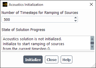
You can re-initialize the acoustics field separately at any time, since it does not influence the transient flow solution which is simply continued further.
You can specify the number of timesteps for the ramping process using the TUI command:
/solve/initialize/init-acoustics-options
Note: If you enable the wave equation model in a non-initialized setup, then the initialization of the entire simulation will also initialize acoustics. However the ramping duration will be set to zero. You can reset the ramping process by re-initializing acoustics separately.
The User Defined Function of the type DEFINE_INIT
DEFINE_INIT cannot be used to
initialize the wave equation model. Please use instead the
DEFINE_ON_DEMAND function DEFINE_ON_DEMAND.
The following field variables are available in the Acoustics… group for post-processing:
Sound Pressure
– main practical interest, connected to the sound potential by Equation 11–12. The sound pressure field is less smooth than the sound potential field because of numerical differentiation.
Sound Potential
– primary solution variable.
Sound DP/Dt
– time derivative of the sound pressure (a second time derivative of the primary solution variable). This field may display a lot of noise.
Sound WaveEq Model Source
– original model source term.
Sound WaveEq Model Source Smoothed
– source term smoothed by the time filter.
Sound WaveEq Model Source Mask
– source masking marker.
Sound Sponge Layer
          Marker
– sponge layer marker.
You can also postprocess results using the Ansys Sound Analysis dialog box. Refer to Postprocessing the FW-H Acoustics Model Data for additional information.
Note: Both the Sound WaveEq Model Source and Sound WaveEq
Model Source Smoothed do not include the effects of source masking and
ramping. In order to see the source field after the application of masking and ramping,
you can use the advanced output field Sound WaveEq Source in the
Acoustics… group, which can be enabled by entering
yes to the following text command:
/solve/set/advanced/retain-temporary-solver-mem.
The Kirchhoff integral model is available for a three-dimensional acoustics simulation with the wave equation model. It is activated by selecting the checkbox, Remote Receivers, in the Acoustics Model dialog box. When this checkbox is selected, a subframe, Kirchhoff Integral Options, with additional buttons appear in the Wave Equation Options frame, as shown in Figure 23.20: Acoustics Model Dialog Box with Kirchhoff Integral Options.
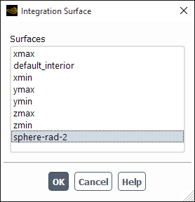
Clicking Integration Surface... opens a list of all currently available surfaces, see an example in Figure 23.21: Integration Surface Dialog Box. The two most useful surface types for the Kirchhoff model are quadric surfaces (ribbon menu Domain→Surface→Create→Quadric) and iso-surfaces. With the current implementation only one surface can be selected in the list and used for the integration.
Clicking Define Receivers... opens the same Acoustic
Receivers dialog box that is used to set up the Ffowcs Williams and Hawkings
(FW-H) model, see Specifying Acoustic Receivers. For convenience, to
simplify the simultaneous use of the FW-H model and the wave equation-based Kirchhoff
integral model, receivers are shared between the two models and do not need to be set up
twice. The signal file name extension for the Kirchhoff model is fixed to
.ark.
Clicking Write Signals writes the computed sound signals at the remote receiver locations to ASCII files. The written Kirchhoff signals are always auto-pruned, see Pruning the Signal Data Automatically for the details. If a sound signal is too short and does not yet contain the complete sound pressure data, then it is not written, and a warning message is printed in the Fluent console.
Important:
The Moving Receivers option is supported only by the FW-H model. In the current implementation of the Kirchhoff model this option is ignored.
The resulting signals are stored in memory and written in the data file separately for the FW-H and Kirchhoff model, which enables their simultaneous use and their comparison. When, however, the sound signals are being written in ASCII receiver files (see entry fields Signal File Name in Figure 23.7: The Acoustic Receivers Dialog Box), both models share the same user-specified file name roots with the different model-specific extensions:
.ardfor the FW-H model signals, and.arkfor the Kirchhoff model signals.
The Kirchhoff model is currently available only in “on-the-fly” mode, which means that the next set of signal samples is computed during a transient simulation after each time step. The “read-and-compute” mode for the FW-H model makes it possible to use the same transient flow simulation for both the FW-H and the wave equation model (with the Kirchhoff integral). To perform such a simulation:
Select the Wave Equation model and mark both the Export Acoustic Source Data in ASD Format and Remote Receivers checkboxes, as shown in Figure 23.20: Acoustics Model Dialog Box with Kirchhoff Integral Options.
Specify integration surfaces for the FW-H model by clicking Define Sources... under the Export Options frame.
Specify an integration surface for the Kirchhoff model by selecting Integration Surface... in the Kirchhoff Integral Options frame.
During a transient flow simulation, at every timestep, the acoustics wave equation will be solved and the sound signals at the remote receivers will be advanced in time using the Kirchhoff integral model. Source data for the FW-H model will also be exported in the ASD format. After the end of the simulation, write the Kirchhoff signals to ASCII files by clicking Write Signals.
Switch to the FW-H model, and then on the Run Calculations task page, start the FW-H model computations with the input from the ASD files using the Acoustic Signals... button. More details about the “read-and-compute” mode of the FW-H model are available in Writing Source Data Files.
The text commands for the Kirchhoff model, which can be used in the Fluent console and in journal files, are shown here in bold.
/define/models/acoustics/wave-equation-options>
basic-shapes/                                   sponge-layer-base-level
remote-receivers-options/                       sponge-layer-factor
remote-receivers?                               sponge-layer-udf
source-mask-udf                                 time-filter-source?
/define/models/acoustics/wave-equation-options/remote-receivers-options>
integration-surface         write-signals