


For background information about the mixture model and the limitations that apply, refer to Overview in the Theory Guide.
For additional information, see the following sections:
Instructions for specifying the necessary information for the primary and secondary phases and their interaction for a mixture model calculation are provided below.
The procedure for defining the primary phase in a mixture model calculation is the same as for a VOF calculation. See Defining the Primary Phase for details.
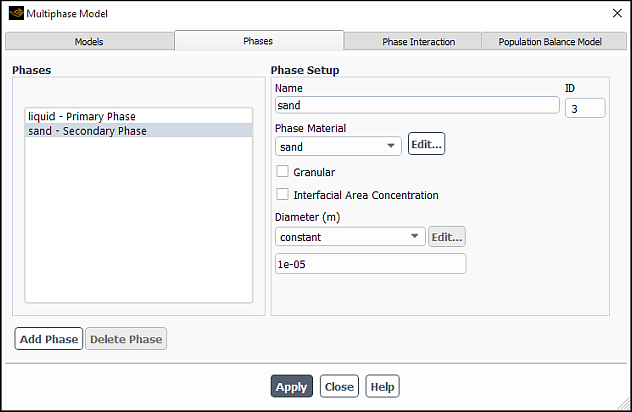
To define a non-granular (that is, liquid or vapor) secondary phase in a mixture multiphase calculation, go to the Phases tab of the Multiphase Model dialog box and perform the following steps:
Select the phase (for example, phase-2) in the Phases list.
In the Phase Setup group box, enter a Name for the phase (for example,
sand).Specify which material the phase contains by choosing the appropriate material in the Phase Material drop-down list.
Define the material properties for the Phase Material, following the same procedure you used to set the material properties for the primary phase (see Defining the Primary Phase). For a particulate phase (which must be placed in the fluid materials category, as mentioned in Steps for Using a Multiphase Model), you need to specify only the density; you can ignore the values for the other properties, since they will not be used.
Specify the Diameter of the bubbles, droplets, or particles of this phase (
 in Equation 14–166 in the Theory Guide). You can specify a
constant value, or use a user-defined function. See the Fluent Customization Manual for details about user-defined functions. Note that when you
are using the mixture model without slip velocity, this input is a characteristic
length scale.
in Equation 14–166 in the Theory Guide). You can specify a
constant value, or use a user-defined function. See the Fluent Customization Manual for details about user-defined functions. Note that when you
are using the mixture model without slip velocity, this input is a characteristic
length scale.Click .
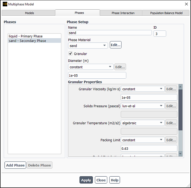
To define a granular (that is, particulate) secondary phase in a mixture model multiphase calculation, perform the following steps:
Select the phase (for example, phase-2) in the Phases list.
In the Phase Setup group box, enter a Name for the phase (for example,
sand).Specify which material the phase contains by choosing the appropriate material in the Phase Material drop-down list.
Define the material properties for the Phase Material, following the same procedure you used to set the material properties for the primary phase (see Defining the Primary Phase). For a granular phase (which must be placed in the fluid materials category, as mentioned in Steps for Using a Multiphase Model), you need to specify only the density; you can ignore the values for the other properties, since they will not be used.
Important: Note that all properties for granular flows can be defined by user-defined functions (UDFs).
See the Fluent Customization Manual for details about user-defined functions.
Enable the Granular option.
Specify the Diameter of the particles. You can select constant in the drop-down list and specify a constant value, or select user-defined to use a user-defined function. See the Fluent Customization Manual for details about user-defined functions.
In the Granular Properties group box, specify the following properties of the particles of this phase:
- Granular Viscosity
specifies the method for computing the kinetic (
 ) and collisional (
 ) components of the granular viscosity (Equation 14–139 in the Fluent Theory Guide). Selecting constant,
syamlal-obrien (Equation 14–141 in the Fluent Theory Guide), or gidaspow (Equation 14–142 in the Fluent Theory Guide) will use these expressions for the kinetic
portion of the viscosity and will calculate the collisional portion of the
viscosity from Equation 14–140 in the Fluent Theory Guide. Alternatively, you can select
user-defined to use a user-defined function. Note that if
you select user-defined, your user-defined function must
include both the kinetic portion and the collisional portion of the viscosity in
the value it returns.
) components of the granular viscosity (Equation 14–139 in the Fluent Theory Guide). Selecting constant,
syamlal-obrien (Equation 14–141 in the Fluent Theory Guide), or gidaspow (Equation 14–142 in the Fluent Theory Guide) will use these expressions for the kinetic
portion of the viscosity and will calculate the collisional portion of the
viscosity from Equation 14–140 in the Fluent Theory Guide. Alternatively, you can select
user-defined to use a user-defined function. Note that if
you select user-defined, your user-defined function must
include both the kinetic portion and the collisional portion of the viscosity in
the value it returns.- Frictional Pressure
specifies the pressure gradient term,
 , in the granular-phase momentum equation. Choose
none to exclude frictional pressure from your
calculation, johnson-et-al to apply Equation 14–371 in the Theory Guide,
syamlal-obrien to apply Equation 14–268 in the Theory Guide, based-ktgf,
where the frictional pressure is defined by the kinetic theory [38]. The solids pressure tends to a large value near the
packing limit, depending on the model selected for the radial distribution
function. You must hook a user-defined function when selecting the
user-defined option. See the Fluent Customization Manual for information on hooking a UDF.
, in the granular-phase momentum equation. Choose
none to exclude frictional pressure from your
calculation, johnson-et-al to apply Equation 14–371 in the Theory Guide,
syamlal-obrien to apply Equation 14–268 in the Theory Guide, based-ktgf,
where the frictional pressure is defined by the kinetic theory [38]. The solids pressure tends to a large value near the
packing limit, depending on the model selected for the radial distribution
function. You must hook a user-defined function when selecting the
user-defined option. See the Fluent Customization Manual for information on hooking a UDF.- Frictional Modulus
is defined as

(26–17)
with
 , which is the derived option. You can
also specify a user-defined function for the frictional
modulus.
, which is the derived option. You can
also specify a user-defined function for the frictional
modulus.- Friction Packing Limit
specifies a threshold volume fraction at which the frictional regime becomes dominant. The default value is 0.61.
- Granular Temperature
specifies temperature for the solids phase and is proportional to the kinetic energy of the random motion of the particles. Choose either the algebraic, the constant, or user-defined option.
- Solids Pressure
specifies the pressure gradient term,
 , in the granular-phase momentum equation. Choose either the
lun-et-al, the syamlal-obrien, the
ma-ahmadi, or the user-defined
option.
, in the granular-phase momentum equation. Choose either the
lun-et-al, the syamlal-obrien, the
ma-ahmadi, or the user-defined
option.- Radial Distribution
specifies a correction factor that modifies the probability of collisions between grains when the solid granular phase becomes dense. Choose either the lun-et-al, the syamlal-obrien, the ma-ahmadi, the arastoopour, or a user-defined option.
- Elasticity Modulus
is defined as

(26–18)
with
 .
.Choose either the derived or user-defined options.
- Packing Limit
specifies the maximum volume fraction for the granular phase. For monodispersed spheres, the packing limit is about 0.63, which is the default value in Ansys Fluent. In polydispersed cases, however, smaller spheres can fill the small gaps between larger spheres, so you may need to increase the maximum packing limit.
Click .
If you want to solve the transport equation for interfacial area concentration of the secondary phase in the mixture model (Interfacial Area Concentration in the Fluent Theory Guide, perform the following steps:
In the Phases tab of the Multiphase Model dialog box, select the phase (for example, phase-2) from the Phases list.
Figure 26.48: The Multiphase Model Dialog Box Displaying the Interfacial Area Concentration Settings
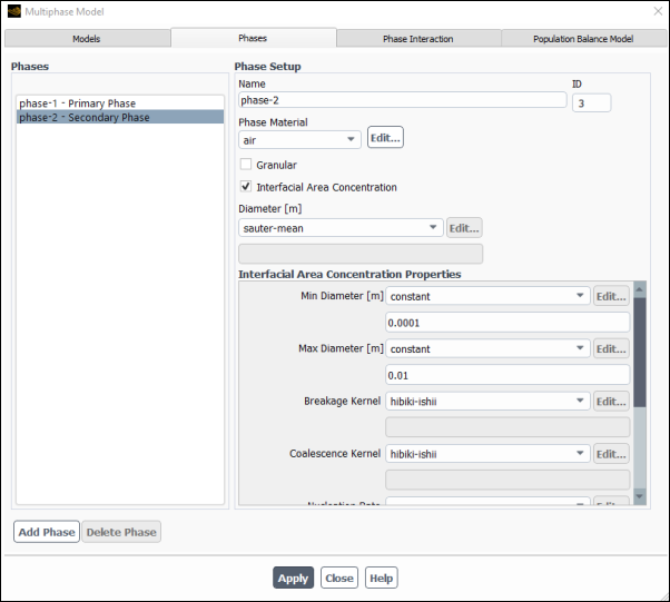
In the Phase Setup group box, enter a Name for the phase (for example,
water-vapor).Specify which material the phase contains by choosing the appropriate material in the Phase Material drop-down list.
Define the material properties for the Phase Material.
Enable the Interfacial Area Concentration option. Make sure the Granular option is disabled for the Interfacial Area Concentration option to be visible in the interface.
Specify the Diameter of the particles or bubbles. You can select constant in the drop-down list and specify a constant value, or select user-defined to use a user-defined function. See the Fluent Customization Manual for details about user-defined functions. The Diameter recommended setting is sauter-mean, allowing for the effects of the interfacial area concentration values to be considered for mass, momentum and heat transfer across the interface between phases.
In the Interfacial Area Concentration Properties group box, specify the following properties of the particles of this phase:
- Min/Max Diameter
are the limits of the bubble diameters.
- Coalescence Kernel, Breakage Kernel
allow you to specify the coalescence and breakage kernels. You can select none, constant, hibiki-ishii, ishii-kim, yao-morel, or user-defined. The three options, hibiki-ishii, ishii-kim and yao-morel are described in detail in Interfacial Area Concentration in the Theory Guide.
In addition to specifying the hibiki-ishii, ishii-kim, and yao-morel as the coalescence and breakage kernels, you can also tune the properties of the three models by using the
/define/phases/iac-expert/hibiki-ishii-model,/define/phases/iac-expert/ishii-kim-model, and/define/phases/iac-expert/yao-morel-modeltext commands.For each of the three models you can specify the parameters listed in Table 26.12: Parameters for the Coalescence and Breakage Kernels
Table 26.12: Parameters for the Coalescence and Breakage Kernels
Hibiki-Ishii Ishii-Kim Model Yao-Morel Model Coefficient Gamma_cCoefficient CrcCoefficient K_c1Coefficient K_cCoefficient CweCoefficient K_c3Coefficient Gamma_bCoefficient CCoefficient K_b1Coefficient K_bCoefficient Ctialpha_maxalpha_maxalpha_max
These values are discussed in greater detail in Interfacial Area Concentration in the Theory Guide.
- Nucleation Rate
is a source term for the interfacial area concentration that models the rate of formation of the dispersed phase. You can choose from constant or user-defined.
- Surface Tension
specifies the surface tension at the liquid-air interface. You can select either the hibiki-ishii or the ishii-kim model.
- Critical Weber Number
will need to be specified if you selected ishii-kim or yao-morel for the Breakage Kernel.
- Dissipation Function
gives you the option to choose the formula which calculates the dissipation rate used in the hibiki-ishii and ishii-kim models. You can choose amongst constant, wu-ishii-kim, fluent-ke, and user-defined for the dissipation function.
The wu-ishii-kim option uses a simple algebraic correlation for
 :
:
(26–19)
where

and

where
 ,
,  ,
,  , and
, and  are the mixture density, mixture velocity, mixture molecular
viscosity, and hydraulic diameter of the flow path.
are the mixture density, mixture velocity, mixture molecular
viscosity, and hydraulic diameter of the flow path.When you select the wu-ishii-kim model, you will set an additional input for Hydraulic Diameter.
- Hydraulic Diameter
is the value used in Equation 26–19, should you use the wu-ishii-kim formulation.
Click Apply.
Note: When solving a steady-state problem, the preferred setting for the
Under-Relaxation Factor is 1.0, as the interfacial area equation
for the boiling models is currently under-relaxed using a locally defined pseudo time
step. If you want extra explicit under-relaxation, you may set the value of the
Under-Relaxation Factor to less than one, this may be done only in
case of serious convergence problems with the interfacial area transport equation. To
improve convergence you can switch to a pseudo time step for the interfacial area
concentration only, using the
define/phases/iac-expert/iac-pseudo-time-step text command and
set the local pseudo time step to less than 1.
If you have chosen not to solve the transport equation for Interfacial Area Concentration as described in Defining the Interfacial Area Concentration via the Transport Equation, then you can select an algebraic model to estimate the interfacial area from the secondary phase diameter specified in the Phases tab of the Multiphase Model dialog box. To choose an algebraic interfacial area model perform these steps.
In the Multiphase Model dialog box, go to the Phase Interaction > Interfacial Area tab.
Select the desired algebraic model from the Interfacial Area drop-down list:
- ia-symmetric
considers both the primary and secondary phase volume fractions in estimating the interfacial area.
- ia-particle
considers the secondary phase volume fraction in estimating the interfacial area.
- ia-gradient
considers the volume fraction gradient at the interface between two phases in estimating the interfacial area.
- ia-hybrid
uses different algebraic interfacial area models for different regimes. This item is available only for the regime flow modeling. See Using the Flow Regime Modeling for more information about this method.
- user-defined
See
DEFINE_EXCHANGE_PROPERTYin the Fluent Customization Manual.
In addition to these models, Ansys Fluent provides the Gradient-Symmetric model, which is available via the text user interface. You can use the following text commands to enable this model:
solve/set/multiphase-numerics/heat-mass-transfer/area-density/ia-grad-sym?
switch to ia-grad-symmetric option? [yes]
yes
See Algebraic Models in the Fluent Theory Guide for details about the theory behind algebraic interfacial area models.
For mixture multiphase flows with slip velocity, you can specify the drag function to be used in the calculation.
To specify drag laws, go to the Phase Interaction > Forces tab in the Multiphase Model dialog box (Figure 26.49: The Multiphase Model Dialog Box for the Mixture Model (Forces Tab)) and make the appropriate selections in the Drag Coefficient group box.
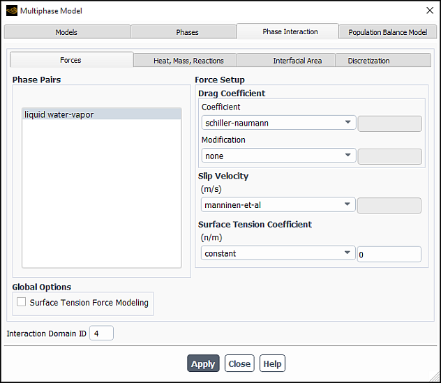
The drag coefficients available here are a subset of those discussed in Specifying the Drag Function.
In addition, for cases that involve flow regime modeling, the drag-hybrid method is available as described in Using the Flow Regime Modeling.
Relative (Slip) Velocity and the Drift Velocity in the Theory Guide provides theoretical background information.
If you are solving for slip velocities during the mixture calculation, you can modify the slip velocity definition in the Phase Interaction > Forces tab in the Multiphase Model dialog box (Figure 26.49: The Multiphase Model Dialog Box for the Mixture Model (Forces Tab)).
Under Slip Velocity, you can specify the slip velocity function for each secondary phase with respect to the primary phase by choosing the appropriate item in the adjacent drop-down list.
Select manninen-et-al (the default) to use the algebraic slip method of Manninen et al. [95], described in Relative (Slip) Velocity and the Drift Velocity in the Theory Guide.
Select none if the secondary phase has the same velocity as the primary phase (that is, no slip velocity).
Select user-defined to use a user-defined function for the slip velocity. See the Fluent Customization Manual for details.
You can include the effects of surface tension along the interface between one or more pairs of phases as described in Including Surface Tension and Adhesion Effects. For more information about the theoretical background, see Surface Tension and Adhesion in the Fluent Theory Guide.
Note:
The surface tension option in recommended for cases with sharp/dispersed interface modeling type.
Jump adhesion is not supported with the Mixture Multiphase model.
If you are solving for slip velocity and using one of the turbulence models in your Mixture multiphase calculation, you can also include the effects of the slip velocity on the momentum and turbulence equations. To include these effects, enable Mixture Drift Force in the Viscous Model Dialog Box. The turbulent dispersion effect will be included in the slip velocity equation (Equation 14–135 in the Fluent Theory Guide). Note that the inclusion of these terms can slow down convergence noticeably. If you are looking for additional accuracy, you may want to compute a solution first without these sources, and then continue the calculation with these terms included. In most cases these terms can be neglected.
The following limitation exists with the flow regime modeling:
The flow regime modeling is supported only with the algebraic slip model, which is valid for low Stokes numbers.
To use the flow regime modeling framework, follow the steps outlined below. Only the steps that are pertinent to the flow regime modeling are listed here. For the theory behind the flow regime modeling, see Flow Regime Modeling in the Fluent Theory Guide.
In the Models tab of the Multiphase Model dialog box, set up the following models and options.
 Setup → Models
→ Multiphase
Setup → Models
→ Multiphase Edit...
In the Model group box, enable Mixture.
In the Model Parameters group box, enable Slip Velocity.
Once you have selected Slip Velocity, the Flow Regime Modeling option appears in the Model Parameters group box.
Enable Flow Regime Modeling.
Once you have enables Flow Regime Modeling, Ansys Fluent automatically enables the following options:
Sharp/Dispersed interface modeling type in the Options group box
Regime Based Discretization in the Interface Modeling Options dialog box.
Note: Although the Dispersed interface modeling type is available, using this option in your simulation may yield less accurate results for some analyses. For instance, the free surface evolution may not be captured well with this option.
Click the button and in the Interface Modeling Options dialog box, specify the appropriate settings.
The default values for both the Bubbly/Droplet Flow Limiter and Free Surface Flow Limiter are 1.5, which should be suitable for most cases. You can modify these values as needed for your analysis. See The Compressive Scheme and Interface-Model-based Variants in the Fluent Theory Guide for more information about the slope limiters.
Click Apply.
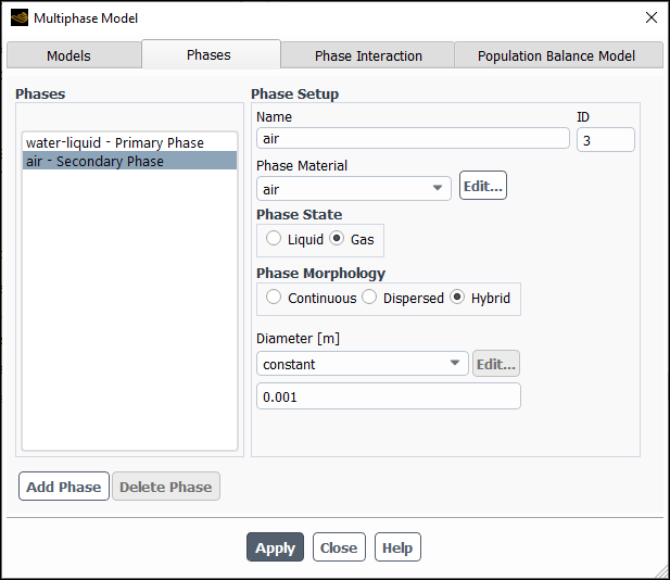
In the Phases tab, define the phases for your simulation.
Define the primary and secondary phases as appropriate.
For each phase, select either Liquid or Gas from the Phase State group box.
Select the Phase Morphology from the following options:
Continuous
Dispersed (available for secondary phases only)
Hybrid
See Flow Regime Modeling in the Fluent Theory Guide for details about phase morphologies.
For phase with either the Dispersed or Hybrid morphology, specify Diameter of the particles, droplets, or bubbles (depending on the flow regime).
Click Apply.
In the Phase Interaction tab, define the interaction between the phases.
For different phase pair interactions, different methods and defaults are available, depending on the phase morphologies. The possible combinations of the phase-pair morphologies are:
Continuous-Continuous
Continuous-Dispersed
Dispersed-Dispersed
Hybrid-Continuous
Hybrid-Dispersed
Hybrid-Hybrid
The methods and default settings available for each phase pair morphology are described below.
In the Forces tab, set the interfacial forces between the phase pairs.
Select the drag coefficient and slip velocity from the Drag Coefficient and Slip Velocity drop-down lists.
The default settings for the drag coefficient and slip velocity for different phase-pair morphology combinations are listed in the table below.
Phase-Pair Morphology Drag Coefficient Slip Velocity Continuous-Continuous
zero-resistance
none
Continuous-Dispersed
schiller-naumann (default)
symmetric
morsi-alexander
ishii-zuber
none
constant
user-defined
manninen-et-al (default)
none
user-defined
Dispersed-Dispersed
-
-
Hybrid-Continuous
Hybrid-Dispersed
Hybrid-Hybrid
drag-hybrid
manninen-et-al (default)
none
user-defined
Note the following:
The zero-resistance method (available only for Continuous-Continuous systems) is equivalent to an infinite drag, which forces the velocities of the continuous phases to be equal. See Phase Pair Interaction for Hybrid Morphology in the Fluent Theory Guide for more information.
If you do not want to consider the drag force or slip velocity, choose none.
The drag-hybrid method uses different drag coefficient methods for different flow regimes. You can select other than the default drag coefficient methods as further described. For more information, see Flow Regime Modeling in the Fluent Theory Guide.
For more information about the drag coefficients, see Defining Drag Between Phases.
For more information about the slip velocity methods, see Defining the Slip Velocity.
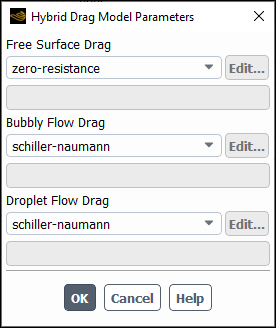
For the drag-hybrid method, you can modify the selection of the drag coefficients for the free surface, bubbly, and droplet flow regimes.
Click next to the selected drag-hybrid drag coefficient.
In the Hybrid Drag Model Parameters dialog box that opens, select the appropriate draft coefficient methods from the Free Surface Drag, Bubbly Flow Drag, and Droplet Flow Drag drop-down lists.
The available methods for different flow regimes are listed in the table below.
Flow Regime Drag Coefficient Free Surface Drag
zero-resistance
Bubbly Flow Drag
Droplet Flow Drag
schiller-naumann (default)
symmetric
morsi-alexander
ishii-zuber
constant
user-defined
Click Apply.
In the Interfacial Area tab, define the interfacial area parameters. See Algebraic Interfacial Area Density Method for Flow Regime Blending in the Fluent Theory Guide for more information.
For each pair of phases, select the interfacial area method.
The available methods for different phase pair morphologies are listed in the table below.
Phase-Pair Morphology Interfacial Area Methods Continuous-Continuous
ia-gradient
user-defined
Continuous-Dispersed
ia-symmetric (default)
ia-particle
user-defined
Dispersed-Dispersed
ia-symmetric (default)
user-defined
Hybrid-Continuous
Hybrid-Dispersed
Hybrid-Hybrid
ia-hybrid
For information about these methods, see Algebraic Models in the Fluent Theory Guide.
For the theory behind the ia-hybrid method, see Algebraic Interfacial Area Density Method for Flow Regime Blending in the Fluent Theory Guide.
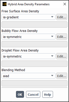
For the ia-hybrid method, you can modify the selection of the area density parameters for the free surface, bubbly, and droplet flow regimes.
Click next to the selected ia-hybrid interfacial area.
In the Hybrid Area Density Parameters dialog box that opens, select the appropriate area density methods from the Free Surface Area Drag, Bubbly Flow Area Density, and Droplet Flow Area Density drop-down lists.
The available methods for different flow regimes are listed in the table below.
Flow Regime Area Density Free Surface Area Density
ia-gradient
user-defined
Blending Method
aiad
user-defined
Select the Blending Method from the following options:
- aiad
is the algebraic interfacial area density (AIAD) method described in Algebraic Interfacial Area Density Method for Flow Regime Blending in the Fluent Theory Guide.
- user-defined
allows you to provide your own blending factors for the flow regime modeling. Refer to
DEFINE_VECTOR_EXCHANGE_PROPERTYin the Fluent Customization Manual for details.
Note: The default values for the AIAD method parameters are suitable for most simulations. If needed, you can adjust these values using the following text commands:
define/models/multiphase/flow-regime-modeling/aiad-parameters/critical-vfSpecifies the critical volume fraction of either gas or liquid for calculating the blending factors for the bubbly and droplet flows (
 and
and  in Equation 14–178 in the Fluent Theory Guide).
define/models/multiphase/flow-regime-modeling/aiad-parameters/delta-gradSpecifies the critical gradient fraction for determining the intermediate transition width for the free surface blending factor (
 in Equation 14–183 in the Fluent Theory Guide).
define/models/multiphase/flow-regime-modeling/aiad-parameters/delta-vfSpecifies the volume fraction width for the intermediate transition (
 in Equation 14–178 in the Fluent Theory Guide).
define/models/multiphase/flow-regime-modeling/aiad-parameters/ncells-fsSpecifies the cell number across the interface for determining the interfacial width for free surface flow (
 in Equation 14–182 in the Fluent Theory Guide).
See Alphabetical Listing of Field Variables and Their Definitions for their definitions.
Click Apply.
Since the algebraic slip model is applicable only to low Stokes number (~1) regimes, you should examine the postprocessing results of the Relaxation Time field variable, which indicates the validity of the algebraic slip model.
The slip velocity treatment is explicit; therefore, lowering the slip velocity under-relaxation factor can improve convergence.
The following additional postprocessing variables will become available for postprocessing under the Phase Interaction... category:
Slip X-velocity
Slip Y-velocity
Slip Z-velocity (3D only)
Flow Regime Blending Factors Fcc, Fcd, Fdc, and Fdd
Relaxation Time
See Field Function Definitions for their definitions.
In addition to the Schnerr-Sauer and Zwart-Gerber-Belamri mechanisms described in Cavitation Mechanism, you can also use the Singhal et al. expert model for special mixture multiphase cases to model the effects of cavitation. For the theory behind this model, refer to Expert Cavitation Model in the Fluent Theory Guide.
The procedure for setting up the Singhal et al. cavitation model is presented below:
Issue the following text command:
solve/set/advanced/singhal-et-al-cavitation-modelEnable? [no]yesEnable the Singhal-Et-Al Cavitation Model option that now appears in the Multiphase Model dialog box under the Phase Interaction > Heat, Mass, Reactions tab.
Specify the following parameters to be used in the calculation of mass transfer due to cavitation:
Vaporization Pressure: The default value of
 is 3540 Pa, the vaporization pressure for water at ambient
temperature. Note that
is 3540 Pa, the vaporization pressure for water at ambient
temperature. Note that  and the surface tension are properties of the liquid, depending
mainly on temperature.
and the surface tension are properties of the liquid, depending
mainly on temperature.Surface Tension Coefficient
Non-Condensable Gas Mass Fraction: The mass fraction of dissolved gases, which depends on the purity of the liquid.
When multiple species are included in one or more secondary phases, or the heat transfer due to phase change must be taken into account, the mass transfer mechanism must be defined before enabling the cavitation model. It may be noted, however, that for cavitation problems, at least two mass transfer mechanisms are defined:
mass transfer from liquid to vapor.
mass transfer from vapor to liquid.
To disable Singhal et al. cavitation model:
Disable the Singhal-Et-Al Cavitation Model option in the Heat, Mass, Reaction tab.
Issue the following text command:
solve/set/advanced/singhal-et-al-cavitation-modelEnable? [yes]no
The semi-mechanistic boiling model can be used only with the following models and conditions:
Mixture multiphase
Turbulent kinetic energy-based models (such as
 -
- or
or  -
- )
) Activated gravity along with zero operating density
Surface tension coefficient (specified in the Phase Interaction > Forces tab of the Multiphase Model dialog box)
Boiling walls with either temperature or conjugate heat transfer boundary conditions
Note: If your case has a boiling wall with heat flux boundary condition, you can add a small thickness of solid and apply heat flux to the solid boundary. Thus you will be able to apply heat flux boundary condition indirectly at the boiling wall through conjugate heat transfer boundary condition.
Binary mixtures with the fixed mixture composition only (pseudo-fluid approach). All the properties and saturation data for the pseudo-fluid must be provided according to the mixture fixed composition.
For the theoretical background on the semi-mechanistic boiling model, see Semi-Mechanistic Boiling Model in the Fluent Theory Guide.
To use the semi-mechanistic boiling model, follow the steps below:
In the Multiphase Model dialog box under the Phase Interaction > Heat, Mass, Reactions tab, specify the Number of Mass Transfer Mechanisms and then select the liquid and vapor phases in the From Phase and To Phase drop-down lists, respectively.
Select evaporation-condensation from the Mechanism drop-down list.
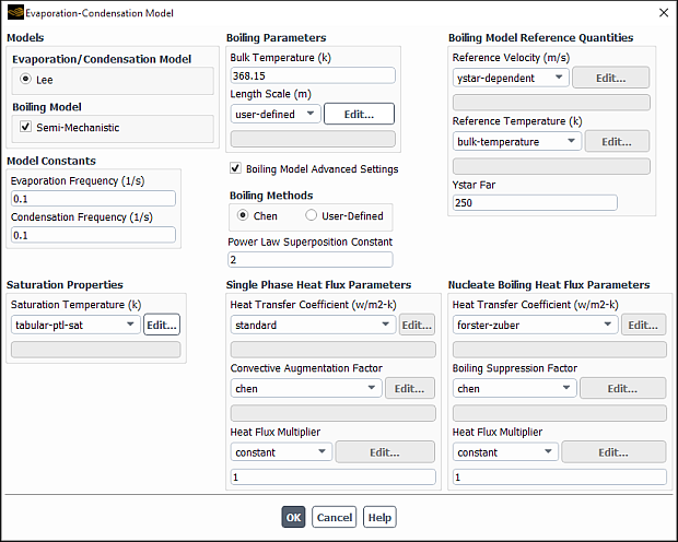
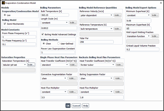
In the Evaporation-Condensation Model dialog box that opens, select Semi-Mechanistic as the Boiling Model.
The Evaporation-Condensation Model dialog box expands to reveal additional Boiling Parameters.
Note: For the Semi-Mechanistic boiling model, the Saturation Temperature can be only specified using either the tabular-pt-sat or tabular-ptl-sat option.
In the Boiling Parameters group box, specify the following parameters:
- Bulk Temperature
is a temperature of bulk fluid away from the wall. Typically, the inlet temperature of the coolant is used as the bulk temperature.
- Length Scale
is used in the calculation of the reference Reynolds number. It is typically taken to be the hydraulic diameter.
To access additional boiling settings for advanced control, select Boiling Model Advanced Settings to reveal more options.
In the Boiling Model Reference Quantities group box, you can specify the following:
- Reference Velocity
is the velocity of the fluid away from a heated wall at some reference location. This quantity is used to calculate the reference Reynolds number
 in Equation 14–639 in the Fluent Theory Guide. You can choose one of the following
specification methods:
in Equation 14–639 in the Fluent Theory Guide. You can choose one of the following
specification methods:- ystar-dependent
(default) calculates the reference velocity away from the boiling wall at
 = 250 using standard wall functions for turbulence.
Here, is a normalized wall distance. You can adjust its value
in the Ystar Far field.
= 250 using standard wall functions for turbulence.
Here, is a normalized wall distance. You can adjust its value
in the Ystar Far field.- constant
specifies a constant value for the reference velocity.
- user-defined
uses a user-defined function for the reference velocity calculation.
- Reference Temperature
is the temperature of fluid away from a heated wall at some reference location (
 in Equation 14–639 in the Fluent Theory Guide). Fluid properties used for the reference
Reynolds number computation are calculated at the reference temperature. You can
choose one of the following specification methods:
in Equation 14–639 in the Fluent Theory Guide). Fluid properties used for the reference
Reynolds number computation are calculated at the reference temperature. You can
choose one of the following specification methods:- bulk-temperature
(default) takes the reference temperature from a user-defined Bulk Temperature value.
- ystar-dependent
calculates the reference temperature at
=250 using standard wall functions for turbulence. In
this case, a value specified for Bulk Temperature
serves as the minimum reference temperature.- user-defined
uses a user-defined function for the reference temperature calculation.
In the Boiling Methods group box, you can select:
- Chen
(default) calculates the boiling heat flux as a weighted superposition of single-phase heat flux (forced convective) and nucleate boiling heat flux. See Semi-Mechanistic Boiling Model in the Fluent Theory Guide for details about this method.
- User-Defined
uses a framework provided by Ansys Fluent to hook user-defined correlations for all of the relevant inputs.
Enter the value for the Power Law Superposition Constant (
 in Equation 14–627 in the Fluent Theory Guide). This constant is used to blend single phase and nucleate boiling heat transfer
coefficients based on asymptotic power law. The default value is 2. The typical range
is from 1 to 3.
in Equation 14–627 in the Fluent Theory Guide). This constant is used to blend single phase and nucleate boiling heat transfer
coefficients based on asymptotic power law. The default value is 2. The typical range
is from 1 to 3.In the Single Phase Heat Flux Parameters group, you can set:
Heat Transfer Coefficient: is
 in Equation 14–628 in the Fluent Theory Guide. The following specifications methods are
available:
in Equation 14–628 in the Fluent Theory Guide. The following specifications methods are
available:standard: Uses a built-in treatment of the heat transfer coefficient for a liquid phase.
constant
user-defined
Convective Augmentation Factor: specifies the single-phase heat flux augmentation factor due to the bubble agitation. The following specification methods are available:
chen: (default) Uses the correlations proposed by Chen. See Semi-Mechanistic Boiling Model in the Fluent Theory Guide for more information.
constant
user-defined
This input parameter is available only when Chen is selected in the Boiling Methods group box.
Heat Flux Multiplier: is an additional factor to adjust a single-phase heat flux (
 in Equation 14–626 in the Fluent Theory Guide). This factor can be used when the single
phase-heat flux is not predicted well due to an under-developed turbulent flow,
uncertainties in surface roughness, interaction of thermal and momentum boundary
layers when starting from different points or other factors. You can choose a
constant or user-defined specification
method. The default value is 1.
in Equation 14–626 in the Fluent Theory Guide). This factor can be used when the single
phase-heat flux is not predicted well due to an under-developed turbulent flow,
uncertainties in surface roughness, interaction of thermal and momentum boundary
layers when starting from different points or other factors. You can choose a
constant or user-defined specification
method. The default value is 1.
In the Nucleate Boiling Heat Flux Parameters group, you can set:
Heat Transfer Coefficient: The specification methods are:
forster-zuber: Uses the nucleate boiling heat transfer coefficient proposed by Forster and Zuber (Equation 14–629 in the Fluent Theory Guide).
constant
user-defined
Boiling Suppression Factor: Accounts for the nucleate boiling suppression due to the effect of forced convection. The presence of bubbles due to local boiling at heated walls augments forced convection and suppresses nucleate boiling. The following specification methods are available:
chen-steiner: (default) Uses the modification proposed by Steiner (Equation 14–635 in the Fluent Theory Guide to Equation 14–637 in the Fluent Theory Guide). See Semi-Mechanistic Boiling Model in the Fluent Theory Guide for more information.
chen: Uses Chen's correlation
 (Equation 14–637 in the Fluent Theory Guide). See Semi-Mechanistic Boiling Model in the Fluent Theory Guide for more information.
constant
user-defined
This input parameter is available only when Chen is selected in the Boiling Methods group box.
Heat Flux Multiplier: is an additional factor to adjust a nucleate boiling heat flux (
 in Equation 14–626 in the Fluent Theory Guide). Boiling correlations are obtained for a specific
pressure and temperature range for certain materials. This additional heat flux
multiplier allows you to tune in heat transfer coefficient when these correlations
are used in generalized sense. You can choose a constant or
user-defined specification method. The default value is
1.
in Equation 14–626 in the Fluent Theory Guide). Boiling correlations are obtained for a specific
pressure and temperature range for certain materials. This additional heat flux
multiplier allows you to tune in heat transfer coefficient when these correlations
are used in generalized sense. You can choose a constant or
user-defined specification method. The default value is
1.
Postprocess the solution results.
When the calculation is complete, the following additional field variables are available in the Wall Fluxes... category.
SMB Single Phase Heat Flux
SMB Nucleate Boiling Heat Flux
You can use the DEFINE_MASS_TR_PROPERTY UDF to define input
parameters for the semi-mechanistic boiling model. See
DEFINE_MASS_TR_PROPERTY
in the Fluent Customization Manual for
details.
By default, boiling is enabled in all the cell zones. When boiling is expected only in certain zones, you can disable boiling in other zones to make the calculation faster. This can be done by clearing Boiling Zone in the Fluid dialog box (Multiphase tab).
You can access expert options for the semi-mechanistic boiling model by issuing the following text commands:
solve/set/multiphase-numerics/heat-mass-transfer/boiling/show-expert-options?
show expert options in semi-mechanistic boiling model? [yes]
yes
The evaporation-condensation model dialog box expands to show boiling model expert options.
You can adjust the following parameters:
- Minimum Superheat
is the minimum superheat required for the onset of nucleate boiling. You can define the Minimum Superheat as:
constant
hsu
user-defined
The hsu method uses the expression proposed by Hsu [67]:
where
 = minimum superheat
 = single phase heat transfer coefficient for
liquid
= single phase heat transfer coefficient for
liquid = thermal conductivity
The remaining notation is the same as in Semi-Mechanistic Boiling Model in the Fluent Theory Guide.
- Maximum Superheat
is the maximum superheat used in the nucleate boiling heat flux expressions.
- Wall Liquid Wetting Fraction
is the area fraction of the wall wetted by liquid. Since a wall may be completely wetted by liquid even if the neighboring cell liquid volume fraction is below 1, this is a crucial parameter for the proper estimation of the heat flux.
You can choose one of the following methods:
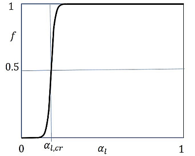
- transition-function
(default) is the wetting fraction that controls the transition from a completely wet to a completely dry wall state. When the liquid volume fraction in the wall neighboring cells exceeds a value of the Critical Liquid Volume Fraction that you specified, the wall is assumed to be completely wetted by liquid. The wetting fraction
 is calculated as:
where
 = volume fraction of liquid
 = Critical Liquid Volume
Fraction (default = 0.2)
= Critical Liquid Volume
Fraction (default = 0.2) = transition constant (default = 20)
The dependency of the wetting function
 on the liquid volume fraction
  is shown in Figure 26.55: Transition Function vs. Volume Fraction of Liquid.
- wall-neighbor
calculates the wetting fraction through the neighboring cell volume fractions.
- constant
allows you to specify the wall liquid wetting fraction as a constant value.
- user-defined
allows you to hook a user-defined function that specifies custom values for the wall liquid wetting fraction.


If you face difficulties in convergence for the energy equation while using the conjugate heat transfer boundary condition, you can use the following strategies:
It is recommended to use meshes with y+ > 5 for better stability.
Use low order schemes for turbulence kinetic energy and momentum.
Reduce the relaxation factor for turbulence kinetic energy to a value between 0.5-0.75.
Reduce the relaxation factor for heat flux to a value between 0.3-0.5.
In case of steady-state simulations that use a pseudo time method with automatic time-scale, reduce the fluid Time Scale Factor to 0.1.
For a large change in heat flux, you can modify the heat flux relaxation factor using the following text command:
solve/set/multiphase-numerics/heat-mass-transfer/boiling/heat-flux-relaxation-factorheat flux relaxation factor for semi-mechanistic boiling model [0.8]0.3The heat flux relaxation factor will be modified as follows:
where
 and
and  are the new and old heat fluxes, respectively, and
  is the heat flux relaxation factor that you specified.

Note: To carry out validations against experimental data, you should first run simulations under non-boiling conditions. If the single-phase heat flux differs from the available data, you should adjust the single-phase heat flux multiplier prior to carrying out the boiling simulations. There is no unique choice of nucleate boiling correlations; therefore, the default nucleate boiling correlation is not guaranteed to work under all the operating conditions. Ansys Fluent provides flexibility either to tune in the existing methods or to hook user-defined properties for all supported boiling model inputs.