


Ansys Fluent can model detailed chemical kinetics in laminar and turbulent flames. Laminar flames are modeled with the Finite-Rate/No TCI option, while four turbulence-chemistry interaction models are available for turbulent flames (Finite-Rate/No TCI, Eddy-Dissipation Concept, Lagrangian PDF Transport, and Eulerian PDF Transport). Detailed chemical mechanisms are invariably numerically stiff and compute-intensive. Ansys Fluent provides following methods to accelerate these computations:
ISAT
Dynamic Mechanism Reduction (DMR)
Chemistry Agglomeration
Dimension Reduction
Dynamic Cell Clustering (DCC) (available with the Ansys CHEMKIN-CFD solver only)
Dynamic Adaptive Chemistry (DAC) (available with the Ansys CHEMKIN-CFD solver only)
All of the methods are enabled or disabled in the Integration Parameters dialog box, accessed from the Species Model dialog box by clicking the Integration Parameters... button in the Reactions group box:
![]() Setup → Models → Species
Setup → Models → Species ![]() Edit...
Edit...
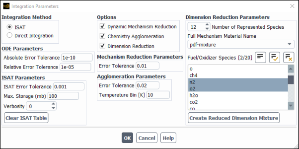
All of the acceleration methods induce some accuracy loss, and the controlling parameters should be carefully adjusted to ensure that this inaccuracy is acceptable, see Chemistry Acceleration in the Fluent Theory Guide. In most cases, applying ISAT and Dynamic Mechanism Reduction (DMR) together should give the best performance. Further information about using the chemistry acceleration models is presented in the following sections:
In-Situ Adaptive Tabulation (ISAT) is a storage-retrieval method that constructs a chemistry table at run time (in-situ) with a user-specified interpolation accuracy (adaptive tabulation). ISAT can be used with all Chemistry solvers except the None - Direct Source solver option. ISAT is not available for simulations with surface reactions.
For ODE solvers (Stiff Chemistry and CHEMKIN-CFD), Ansys Fluent uses two error tolerances (under ODE Parameters):
Absolute Error Tolerance: by default, set to 10-8.
Relative Error Tolerance: by default, set to 10-9 for the Stiff Chemistry solver and 10-4 for the CHEMKIN-CFD solver.
The default values should be sufficient for most applications, although these tolerances may need to be decreased for some cases such as ignition. For problems in which the accuracy of the chemistry integrations is crucial, it may be useful to test the accuracy of the error tolerances in simple zero-dimensional and one-dimensional test simulations with parameters comparable to those in the full simulation.
If you want to use chemistry agglomeration together with ISAT, enable Chemistry
Agglomeration in the Integration Parameters dialog box and
specify the chemistry agglomeration Error Tolerance ( ). More information can be found in Using Chemistry Agglomeration.
For additional information, see the following sections:
If you have selected ISAT under Integration Method, you will then be able to set additional ISAT parameters. The numerical error in the ISAT table is controlled by the ISAT Error Tolerance under ISAT Parameters. The default ISAT Error Tolerance of 0.001 may be sufficiently accurate for temperature and major species, but will most likely need to be decreased to get accurate minor species and pollutant predictions. For steady-state simulations, it may help to start with a high error tolerance during the initial iterations towards a converged solution. A larger error tolerance results in smaller tables and quicker run times, but greater error.
Important: After your steady simulation is converged, you should always decrease the ISAT Error Tolerance and perform further iterations until the species that you are interested in are unchanged.
The Max. Storage is the maximum RAM used by the ISAT table, and has a default value of 100 MB. Generally, you do not need to set it to a value larger than 500 MB. The value of Verbosity allows you to monitor ISAT performance in different levels of detail. See Monitoring ISAT for details about this parameter.
To purge the ISAT table, click the button. See Using ISAT Efficiently for more details.
You can monitor ISAT performance by setting the Verbosity in the
Integration Parameters dialog box. For a Verbosity of
1 or 2, Ansys Fluent writes the following information periodically to a file named
case_file_name_stats.out:
total number of queries
total number of queries resulting in retrieves
total number of queries resulting in grows
total number of queries resulting in adds
total number of queries resulting in direct integrations
cumulative CPU seconds in ISAT
cumulative CPU seconds outside ISAT
cumulative wall-clock time in seconds (that is, total CPU time in ISAT plus total CPU time out of ISAT plus CPU idle time)
The ISAT Verbosity option of 2 is for expert users who are familiar with ISAT v5.0 [123]. Ansys Fluent writes out the following files for Verbosity = 2:
table_name
_stats.out, as described abovetable_name
_ODE_accuracy.outreports the accuracy of the ODE integrations. For every new ISAT table entry, if the maximum absolute error in temperature or species is greater than any previous error, a line is written to this file. This line consists of the total number of ODE integrations performed up to this time, the maximum absolute species error, the absolute temperature error, the initial temperature and the time step.table_name
_ODE_diagnostic.outprints diagnostics from the ODE solvertable_name
_ODE_warning.outprints warnings from the ODE solver
Initially, the table name is equal by default to the current case name, and is changed as the table is written or read.
Each processor builds its own ISAT table. If Verbosity is enabled, each compute node writes out the Verbosity file(s) with the node ID number appended to the file name.
Efficient use of ISAT requires thoughtful control. What follows are some detailed recommendations concerning the achievement of this goal.
Important:
The numerical error in the ISAT table is controlled by the ISAT Error Tolerance, which has a default value of 0.001. This value is relatively large, which allows faster convergence times for steady-state simulations. However, once the solution has converged, it is important to reduce this ISAT Error Tolerance and re-converge. This process should be repeated until the species that you are interested in modeling are unchanged. Unsteady simulations should be run with a sufficiently small ISAT Error Tolerance so that the species of interest are unaffected by this parameter. Note that as the error tolerance is decreased, the memory and time requirements to build the ISAT table will increase substantially. There is a large performance penalty in specifying an error tolerance smaller than is needed to achieve acceptable accuracy, and the error tolerance should be decreased gradually and judiciously.
As described in Mesh Partitioning and Load Balancing, you can select portions of the simulation to consider when performing dynamic load balancing in multiprocessor simulations. If the ISAT option is selected in the Weighting tab of the Partitioning and Load Balancing Dialog Box, the time required for solving chemistry will be factored in when assigning the computational cells to each available processor. It is recommended that you select this option when solving stiff chemistry, particularly when the Dynamic Mechanism Reduction method is enabled; thus, more resources can be allocated for the cells with the larger mechanisms.
During the initial iterations, before a steady-state solution is attained, transient
composition states occur that are not present in the steady-state solution. For example, you
might patch a high temperature region in a cold fuel-air mixing zone to ignite the flame,
whereas the converged solution never has hot reactants without products. Since all states that
are realized in the simulation are tabulated in ISAT, these initial mappings are wasteful of
memory, and can degrade ISAT performance. If the table fills the allocated memory and contains
entries from an initial transient that are no longer accessed, it may be beneficial to purge the
ISAT table. This is achieved by either clearing it in the Integration
Parameters dialog box, or saving your case and data files, exiting Ansys Fluent, then
restarting Ansys Fluent and reading in the case and data. This can also be done with the TUI
command define/models/species/clear-isat-table.
From experience, ISAT performs very well on premixed turbulent flames, where the range of composition states are smaller than in non-premixed flames. ISAT performance degrades in flames with large residence times, where more work is required in the ODE integrator.
Ansys Fluent can write and subsequently read ISAT tables. However, it is in general not recommended to write and read ISAT tables for the following reason: ISAT tabulates chemical states that are specific to a single simulation. The ISAT tabulated composition states are determined by the geometry, boundary conditions, physics models such as turbulence and radiation, thermodynamic and transport properties, as well the chemical mechanism. If any of these parameters change, the realized composition space changes, and significant parts of the existing ISAT table are no longer accessed. These un-accessed ISAT table entries slow interpolation and decrease the number of useful accessed table entries that can be added. Since the time consumed building the ISAT table is typically much smaller than simulation run times, it is advised to rebuild the table when restarting.
When Ansys Fluent is run in parallel, each partition builds its own ISAT table and does not exchange information with ISAT tables on other compute nodes. You can save the ISAT tables on all compute nodes:
![]() File → Write →
ISAT Table...
File → Write →
ISAT Table...
Each compute node writes out its ISAT table to the specified file name, with the node ID
number appended to the file name. For example, a specified file name of
my_name on a two compute node run will write two files called
my_name-0.isat and my_name-1.isat.
Subsequent runs can start from existing ISAT tables by reading them into memory.
![]() File → Read →
ISAT Table...
File → Read →
ISAT Table...
Files can be read in two ways:
Parallel nodes can read in corresponding ISAT tables saved from a previous parallel simulation. The appended node ID should not be removed from the input file name.
Note: The ability to use ISAT tables generated from a parallel simulation with a different number of parallel nodes is not supported.
All nodes can read one unique ISAT table. You might use this approach if you have a large table from a serial simulation. Ansys Fluent first checks to see if the exact file name that you specified exists, and if it does, all nodes will read this one file.
Computational time increases with the size of the chemical kinetics mechanism used in the simulation. Dynamic Mechanism Reduction (DMR) decreases the mechanism size at each cell (or particle) to include only those species and reactions necessary for accurate modeling (within defined tolerances) of the chemical kinetics at the local conditions. This is performed at every flow iteration (for steady simulations) or time step (for transient simulations). Because the mechanism is only required to be accurate at the local conditions, smaller reduced mechanisms can be used with less accuracy loss than when using skeletal mechanism reduction, where a single reduced mechanism is used throughout the simulation. The speed-up from this approach is problem-dependent, but on average is about a factor of two or more compared to a case with no chemistry acceleration.
For an even greater increase in performance, you can use Dynamic Mechanism Reduction with any combination of the other chemistry acceleration options available in Ansys Fluent. In most cases, applying ISAT and DMR together should give the best performance. Note, however, that ISAT performance degrades when accuracy requirements are very strict or when conditions are not revisited often in a simulation. An example is unsteady ignition simulations, where ISAT table entries may not be re-used. However, the important species and reactions can vary widely during the simulation; for example, many of the low temperature ignition reactions are only required for the small spark zone and short spark duration. In such situations, you may achieve better performance using Dynamic Mechanism Reduction along with direct integration method rather than ISAT.
Combining multiple chemistry acceleration methods, however, compounds accuracy loss, since each of these methods accelerates the simulation by sacrificing some accuracy. In general, greater speed-up is achievable when the full mechanism is larger, because there is potential for a greater degree of reduction.
Important: When using Dynamic Mechanism Reduction along with ISAT, setting the error tolerance for either approach above its default value degrades accuracy faster than when either method is used alone.
Dynamic Mechanism Reduction is performed using the Directed Relation Graph (DRG) algorithm. For details of the DMR algorithm, refer to the discussion in Dynamic Mechanism Reduction in the Fluent Theory Guide.
You can enable Dynamic Mechanism Reduction through either the graphical user interface (GUI) or the text user interface (TUI) as follows.
In the GUI, enable the Dynamic Mechanism Reduction option in the Integration Parameters dialog box.
In the TUI, enter the following text command in the console:
define/models/species/integration-parametersWhen prompted with
Enable Dynamic Mechanism Reduction?, answer withyes.Note that it is not necessary to enable Chemistry Acceleration Expert mode in order to use Dynamic Mechanism Reduction.
For additional information, see the following sections:
In Ansys Fluent, Dynamic Mechanism Reduction is controlled by the error tolerance and the target species list, as described below.
- Error Tolerance
(
 in Equation 7–172 in the Fluent Theory Guide).The
default value for error tolerance
in Equation 7–172 in the Fluent Theory Guide).The
default value for error tolerance  is
is 0.01, which should work well for most simulations, balancing speed and accuracy. However, a larger tolerance may be sufficient for some simulations (for example, steady-state simulations with moderate accuracy requirements), while a smaller tolerance may be required in other cases with stricter accuracy requirements (for example, modeling auto-ignition delay times for a highly complex fuel). In general, a larger tolerance yields faster, but less accurate simulations.The error tolerance can be adjusted through the GUI or TUI as follows:
In the GUI, set Error Tolerance to the desired value in the Mechanism Reduction Parameters group box in the Integration Parameters dialog box.
In the TUI, enter the following text command:
define/models/species/integration-parameters. When prompted withMechanism Reduction Error Tolerance, enter the desired tolerance (a positive, nonzero value) or press Enter to retain the default value.
Note:In the TUI, you can also enable Chemistry Acceleration Expert mode, other chemistry acceleration methods, and specify ODE integrator parameters (see Using ISAT for details about these parameters).
Chemistry Acceleration Expert mode should only be enabled if you want to modify the default target species list.
- Target Species List
As described in the Dynamic Mechanism Reduction in the Fluent Theory Guide, the target species are those species that you want to predict most accurately. The default number of target species
 is 3. The first default target species is hydrogen radical. DRG will add
two other species with the largest mass fractions to complete the target species list at each
flow time step or iteration. DRG will then identify all other species that must also be
included in the mechanism in order to accurately model these targets.
is 3. The first default target species is hydrogen radical. DRG will add
two other species with the largest mass fractions to complete the target species list at each
flow time step or iteration. DRG will then identify all other species that must also be
included in the mechanism in order to accurately model these targets.Although you should rarely need to alter the default target species list, Ansys Fluent provides an option to specify target species of your choice. The designated target species can be specified only in the TUI when Chemistry Acceleration Expert mode is enabled. Enter the text command
define/models/species/integration-parametersand then answeryeswhen prompted withEnable Chemistry Acceleration expert?.
Ansys Fluent provides the ability to explicitly specify target species. From your mixture
material list, you can select any number  of target species to be included in the kinetics mechanism. In case no targets
were selected (
of target species to be included in the kinetics mechanism. In case no targets
were selected ( ) or the number of user-selected targets
  is less than the minimum number of target species
  (
( ), the DRG algorithm will add the (
 ) species with the largest mass fractions to the target species list.
As discussed in the Dynamic Mechanism Reduction in the Fluent Theory Guide, there is an option to remove a species from the target list whenever its mass fraction is below a specified threshold. This option is disabled by default in Ansys Fluent (that is, the default value for minimum mass fraction is 0).
When specifying Target Species List, you will receive the following prompts in the console:
Minimum number of target species [3]Enter the desired number of targets.
Minimum mass fraction of target species [0]Enter minimum allowable target mass fraction.
The current target species list will be displayed in the console window (for example, the console output for the default target species consisting of hydrogen radical will be
Current target species list = (h)).Enter target species list...Species name [""]Enter target species name, for example,
"ch4".Important: You must enter the complete name of the species as it appears in the Chemical Formula field in the Create/Edit Materials dialog box within quotes (" ").
After you enter the first target species, you will be prompted to specify the second one, and so on, until you press Enter to complete the setup.
Note, that if you have entered
0for the minimum number of target species and have not provided any target species (that is, the number of
user-selected targets,
and have not provided any target species (that is, the number of
user-selected targets,  , is zero), Ansys Fluent will automatically select the three species with the
largest mass fraction and use them as the target species in the DRG algorithm.
, is zero), Ansys Fluent will automatically select the three species with the
largest mass fraction and use them as the target species in the DRG algorithm.
When Chemistry Acceleration expert is enabled in the TUI, two additional field variables are available to be monitored or examined in postprocessing:
DRG Reduced Number of Species in the Species… category
DRG Reduced Number of Reactions in the Reactions... category
These field variables quantify the size of the reduced mechanism at each cell or particle in the domain (the number of retained species and reactions, respectively).
When you use DMR in combination with ISAT, Ansys Fluent will report values of zero for DRG Reduced Number of Species and DRG Reduced Number of Reactions for those cells where the Ansys solver computed the solution using table lookup instead of direct integration in the ISAT algorithm. A cell value of zero DRG Reduced Number of Species does not imply that the DMR algorithm eliminated all species from the mechanism; rather, it indicates that the Ansys solver performed ISAT table lookup to obtain the chemistry solution at the cell.
If you want to view the cells for which ISAT table lookup was performed in the last iteration or time step, display the DRG Reduced Number of Species plot clipped to a range of 0 to 0. (Make sure that the Node Value option is deselected in the postprocessing dialog boxes.)
If you want to view the cells for which DMR was performed in the last iteration or time step, display the DRG Reduced Number of Species plot clipped to a range of 1 to a global maximum value (as it appears in the Max field when Global Range is selected in the postprocessing dialog boxes).
Note: The DMR postprocessing field variables are not stored in the data file and, hence, will not be available for postprocessing in the next session. If you want to postprocess these variables in your next session, read the data file and perform a single iteration or time step (for steady-state or transient simulations, respectively) in order for the DMR data to be calculated and available for viewing.
As described in Dynamic Mechanism Reduction in the Fluent Theory Guide, mechanism reduction is performed at each cell or particle, once per time step (for transient simulations) or per flow iteration (for steady-state simulations). It is assumed that the reduced mechanism created for the starting conditions will remain valid for the entire transport time step over which the chemistry ODE is integrated. If the chemistry integration time interval is very large, the chemical state can change significantly, degrading the accuracy of the reduced mechanism. In some cases (particularly transient simulations such as ignition) it may be necessary to enforce smaller flow time steps in order to effectively use Dynamic Mechanism Reduction. In this way the reduced mechanisms are updated more frequently to match the changing chemical states.
Note that Dynamic Mechanism Reduction works best when there are significant regions in a computational domain and/or times during a simulation with relatively low chemical activity (for example, low temperature, low mixing of fuel/oxidizer, low concentrations of reactive species, and so on). Consider a simple opposed flow diffusion flame problem with pure fuel as one stream and pure oxygen as the other stream. Large mechanisms (which, depending on the error tolerance, may be close to the full mechanism size) will likely be used in the mixing region where the flame is located, while smaller mechanisms would be used elsewhere in the domain. You should not expect much speed-up if a very large fraction of your grid cells (for example, 90%) are in the flame region.
In steady-state simulations, you can improve the solution time by first running to
convergence with a larger error tolerance  , and then restarting the simulation repeatedly, gradually decreasing the error
tolerance
, and then restarting the simulation repeatedly, gradually decreasing the error
tolerance  until you reach the desired accuracy level. For example, if you first converge
the solution with the error tolerance
until you reach the desired accuracy level. For example, if you first converge
the solution with the error tolerance  , then iterate the solution further to convergence with the lower error
tolerance,
, then iterate the solution further to convergence with the lower error
tolerance,  , and then with the desired error tolerance
  , you will generally be able to achieve faster convergence than iterating from
initial conditions with the error tolerance
, you will generally be able to achieve faster convergence than iterating from
initial conditions with the error tolerance  .
.
Important: As described in Mesh Partitioning and Load Balancing, you can select portions of the simulation to consider when performing dynamic load balancing in multiprocessor simulations. When using the Dynamic Mechanism Reduction along with ISAT, it is recommended that you select the ISAT option in the Weighting tab of the Partitioning and Load Balancing Dialog Box when solving stiff chemistry. If ISAT is selected, the time required for solving chemistry will be factored in when assigning the computational cells to each available processor; thus, more resources can be allocated for the cells with the larger mechanisms.
The Chemistry Agglomeration method reduces the number of calls
to the computationally expensive ODE integrator by clustering cells
with similar compositions. The size of these clusters is determined
by the agglomeration parameters Error Tolerance ( ) and Temperature Bin (
 ) in the Integration Parameters dialog box. Larger values of
  and
and  result in a larger number of agglomerated cells,
fewer calls to the reaction integrator, increased run-time speed,
but greater error.
result in a larger number of agglomerated cells,
fewer calls to the reaction integrator, increased run-time speed,
but greater error.
You can also set the chemistry agglomeration parameters using
the text user interface (TUI) command define/models/species/integration-parameters. Once you enable agglomeration chemistry, Ansys Fluent prompts you for Agglomerate Chemistry Error Tolerance and Agglomerate Chemistry Temperature Bin. Enter the desired
values or press Enter to retain the default values
of 0.02 for Agglomerate Chemistry
Error Tolerance and 10 for Agglomerate Chemistry Temperature Bin.
More information can be found in Chemistry Agglomeration in the Fluent Theory Guide.
Important: The solution accuracy can be improved by decreasing the tolerances. Generally, it should not be necessary to reduce the tolerances below 0.01 and 10 K.
Detailed kinetic mechanisms typically contain a multitude of intermediate species that far exceed the number of major fuel, oxidizer, and product species. Chemical mechanism Dimension Reduction reduces the number of intermediate species transport equations (called representative species) that are solved, and reconstructs the ‘unrepresented’ species using chemical equilibrium assumptions.
Important: Since Ansys Fluent is limited to a maximum of 700 transported species, the main use of Dimension Reduction is to enable simulation with chemical mechanisms containing more than 700 species.
Follow these steps to use Dimension Reduction:
Import your CHEMKIN mechanism. Note that you can import CHEMKIN mechanisms that contain more than 700 species.
Click the button in the Species Model dialog box, and enable Dimension Reduction.
Set the Number of Represented Species. This must be greater than 10 and less than the number of species in the full mechanism. The Number of Represented Species must also be less than 700 minus the number of unrepresented elements (the number of chemical elements in the unrepresented species). A larger Number of Represented Species will increase accuracy, but also increase computational expense. The default of 12 has been chosen to provide a good compromise between accuracy and speed.
Select the Full Mechanism Material Name, which is typically the name of the CHEMKIN mechanism that you imported. Ansys Fluent can store several imported CHEMKIN mechanisms in different mixture materials whose mechanisms you are not using. However, since mechanisms are typically large, you should delete unused mixtures to reduce memory requirements.
Set the boundary and initial fuel and oxidizer, as well as product species, as represented species. These are set in the Fuel/Oxidizer Species list. Note that you can force other species to be represented by selecting them here. Species of interest, especially species that are not near chemical equilibrium, such as pollutants, and their associated intermediate species in the mechanism should also be included. Intermediate species that occur in large mass fractions relative to the fuel and oxidizer species should be included, as well as species important in the chemical pathway. For example, for methane combustion in air, CH3 should be included as a represented species since CH4 pyrolizes to CH3 first.
Click . This will create a new mixture material called
reduced-dimension-mixture, which contains the represented species as well as proxy ’species’ for the unrepresented elements. These unrepresented elements have “u" prepended to the element name. You should never rename the reduced-dimension-mixture mixture material, or select another mixture as the active material, while Dimension Reduction is enabled.Continue with the setup, solution, and postprocessing as for other detailed chemistry cases. Note that the boundary and initial mass fraction of unrepresented elements should always be zero. The entries for the unrepresented element mass fractions are disabled in the Ansys Fluent GUI.
For postprocessing, the unrepresented elements are available in the Species list as the element name with “u" prepended. All species in the full mechanism, consisting of both represented and unrepresented species, are available in the Full Mechanism Species... category of the postprocessing dialog boxes.
After you obtain a preliminary solution with Dimension Reduction, it is recommended that you check the magnitude of all unrepresented species, which are available in the Full Mechanism Species... option in the Contours dialog box. If the mass fraction of any unrepresented species is larger than other represented species, you should repeat the simulation with this species included in the represented species list. In turn, the mass fraction of all unrepresented elements should decrease.
Note: Note that Dimension Reduction is only available with ISAT. Dimension Reduction is initially comparable in speed to a simulation with the full mechanism, but iterations become significantly faster at later times when the ISAT table is populated.
For information about the theory of this option, see Chemical Mechanism Dimension Reduction in the Fluent Theory Guide.
The Dynamic Cell Clustering (DCC) method is available with the Ansys CHEMKIN-CFD solver. DCC groups computational cells with similar temperatures, pressures, and initial species mass fractions into clusters.
To use the DCC method, select Dynamic Cell Clustering in the Integration Parameters dialog box.
The following parameters are available for controlling dynamic cell clustering:
Max. Temperature Dispersion (default =10 K)
Max. Equiv. Ratio Dispersion (default =0.05)
Max. Clusterization (default = 10) and Min. Clusterization (default = 0)
These parameters limit the number of generated clusters and allocate the required amount of memory in your analysis.
Reactants Threshold (mass fraction) (default = 1e-09)
If the computed value of the species mass fraction is above the specified threshold, then the solver calculates the clusterization parameters; otherwise, it is considered to be zero.
The default values for these parameters have been found to provide accurate results for a wide range of combustion cases. Varying these parameters may affect the computational cost. For example, reducing maximum temperature and equivalence ratio of dispersions increases the number of clusters, which leads to a higher CPU cost.
For background information about DCC, refer to Dynamic Cell Clustering with Ansys Fluent CHEMKIN-CFD Solver in the Fluent Theory Guide.
Note: Dynamic Adaptive Chemistry is not compatible with ISAT.
The Dynamic Adaptive Chemistry method is controlled by the following parameters:
DAC Error Tolerance: Controls the level of accuracy.
A larger tolerance would tend to lower the accuracy but might speed up the computation. The default value for DAC error tolerance is 0.001, which should be suitable for most cases.
DAC target species: Are the initial species to be tracked by the DAC algorithm.
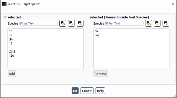
You can select the target species for your analysis in the Select DAC Target Species dialog box that opens when you click in the Integration Parameters dialog box.
For both diesel and gasoline surrogate fuels, CO, HO2, and fuel species are an effective choice for the target species (367 and 368). By default, only co and ho2 are selected as the DAC target species. You must also select fuel species for your analysis.
To modify the DAC target species list:
To remove the species from the Selected Species multiple-selection list, select it and click . The species will be moved from the Selected Species list to the Unselected Species list.
To add the species back to the Selected Species list, select it in the Unselected Species multiple-selection list and click . The species will be moved from the Unselected Species list to the Selected Species list.
For information about the theory of this method, see Dynamic Adaptive Chemistry with Ansys Fluent CHEMKIN-CFD Solver in the Fluent Theory Guide.