


The tracking of the interface(s) between the phases is accomplished
by the solution of a continuity equation for the volume fraction of
one (or more) of the phases. For the  phase,
this equation has the following form:
phase,
this equation has the following form:
 | (14–8) |
where  is
the mass transfer from phase
is
the mass transfer from phase  to phase
  and
and  is
the mass transfer from phase
is
the mass transfer from phase  to phase
  . By default, the source term on the right-hand side
of Equation 14–8,
. By default, the source term on the right-hand side
of Equation 14–8,  , is zero, but you can
specify a constant or user-defined mass source for each phase. See Modeling Mass Transfer in Multiphase Flows for more information
on the modeling of mass transfer in Ansys Fluent’s general multiphase
models.
, is zero, but you can
specify a constant or user-defined mass source for each phase. See Modeling Mass Transfer in Multiphase Flows for more information
on the modeling of mass transfer in Ansys Fluent’s general multiphase
models.
The volume fraction equation will not be solved for the primary phase; the primary-phase volume fraction will be computed based on the following constraint:
 | (14–9) |
The volume fraction equation may be solved either through implicit or explicit time formulation.
When the implicit formulation is used, the volume fraction equation is discretized in the following manner:
 | (14–10) |
|
where: | |
|
| |
|
| |
|
| |
|
| |
|
| |
|
| |
|
|


Since the volume fraction at the current time step is a function of other quantities at the current time step, a scalar transport equation is solved iteratively for each of the secondary-phase volume fractions at each time step.
Face fluxes are interpolated using the chosen spatial discretization scheme. The schemes available in Ansys Fluent for the implicit formulation are discussed in Spatial Discretization Schemes for Volume Fraction in the User's Guide.
The implicit formulation can be used for both time-dependent and steady-state calculations. See Choosing Volume Fraction Formulation in the User's Guide for details.
The explicit formulation is time-dependent and the volume fraction is discretized in the following manner:
 | (14–11) |
|
where | |
|
| |
|
| |
|
| |
|
| |
|
|


Since the volume fraction at the current time step is directly calculated based on known quantities at the previous time step, the explicit formulation does not require and iterative solution of the transport equation during each time step.
The face fluxes can be interpolated using interface tracking or capturing schemes such as Geo-Reconstruct, CICSAM, Compressive, and Modified HRIC (See Interpolation Near the Interface). The schemes available in Ansys Fluent for the explicit formulation are discussed in Spatial Discretization Schemes for Volume Fraction in the Fluent User's Guide.
Ansys Fluent automatically refines the time step for the integration of the volume fraction equation, but you can influence this time step calculation by modifying the Courant number. You can choose to update the volume fraction once for each time step, or once for each iteration within each time step. These options are discussed in more detail in Setting Time-Dependent Parameters for the Explicit Volume Fraction Formulation in the Fluent User's Guide.
Important: When the explicit scheme is used, a time-dependent solution must be computed.
Ansys Fluent’s control-volume formulation requires that convection and diffusion fluxes through the control volume faces be computed and balanced with source terms within the control volume itself.
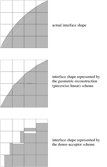
In the geometric reconstruction and donor-acceptor schemes, Ansys Fluent applies a special interpolation treatment to the cells that lie near the interface between two phases. Figure 14.2: Interface Calculations shows an actual interface shape along with the interfaces assumed during computation by these two methods.
The explicit scheme and the implicit scheme treat these cells with the same interpolation as the cells that are completely filled with one phase or the other (that is, using the standard upwind (First-Order Upwind Scheme), second-order (Second-Order Upwind Scheme), QUICK (QUICK Scheme), modified HRIC (Modified HRIC Scheme), compressive (The Compressive Scheme and Interface-Model-based Variants), or CICSAM scheme (The Compressive Interface Capturing Scheme for Arbitrary Meshes (CICSAM)), rather than applying a special treatment.
In the geometric reconstruction approach, the standard interpolation schemes that are used in Ansys Fluent are used to obtain the face fluxes whenever a cell is completely filled with one phase or another. When the cell is near the interface between two phases, the geometric reconstruction scheme is used.
The geometric reconstruction scheme represents the interface between fluids using a piecewise-linear approach. In Ansys Fluent this scheme is the most accurate and is applicable for general unstructured meshes. The geometric reconstruction scheme is generalized for unstructured meshes from the work of Youngs [728]. It assumes that the interface between two fluids has a linear slope within each cell, and uses this linear shape for calculation of the advection of fluid through the cell faces. (See Figure 14.2: Interface Calculations.)
The first step in this reconstruction scheme is calculating the position of the linear interface relative to the center of each partially-filled cell, based on information about the volume fraction and its derivatives in the cell. The second step is calculating the advecting amount of fluid through each face using the computed linear interface representation and information about the normal and tangential velocity distribution on the face. The third step is calculating the volume fraction in each cell using the balance of fluxes calculated during the previous step.
Important: When the geometric reconstruction scheme is used, a time-dependent solution must be computed. Also, if you are using a conformal mesh (that is, if the mesh node locations are identical at the boundaries where two subdomains meet), you must ensure that there are no two-sided (zero-thickness) walls within the domain. If there are, you will need to slit them, as described in Slitting Face Zones in the User's Guide.
In the donor-acceptor approach, the standard interpolation schemes that are used in Ansys Fluent are used to obtain the face fluxes whenever a cell is completely filled with one phase or another. When the cell is near the interface between two phases, a "donor-acceptor" scheme is used to determine the amount of fluid advected through the face [249]. This scheme identifies one cell as a donor of an amount of fluid from one phase and another (neighbor) cell as the acceptor of that same amount of fluid, and is used to prevent numerical diffusion at the interface. The amount of fluid from one phase that can be convected across a cell boundary is limited by the minimum of two values: the filled volume in the donor cell or the free volume in the acceptor cell.
The orientation of the interface is also used in determining
the face fluxes. The interface orientation is either horizontal or
vertical, depending on the direction of the volume fraction gradient
of the  phase within
the cell, and that of the neighbor cell that shares the face in question.
Depending on the interface’s orientation as well as its motion,
flux values are obtained by pure upwinding, pure downwinding, or some
combination of the two.
phase within
the cell, and that of the neighbor cell that shares the face in question.
Depending on the interface’s orientation as well as its motion,
flux values are obtained by pure upwinding, pure downwinding, or some
combination of the two.
Important: When the donor-acceptor scheme is used, a time-dependent solution must be computed. Also, the donor-acceptor scheme can be used only with quadrilateral or hexahedral meshes. In addition, if you are using a conformal mesh (that is, if the mesh node locations are identical at the boundaries where two subdomains meet), you must ensure that there are no two-sided (zero-thickness) walls within the domain. If there are, you will need to slit them, as described in Slitting Face Zones in the User's Guide.
The compressive interface capturing scheme for arbitrary meshes (CICSAM), based on Ubbink’s work [662], is a high resolution differencing scheme. The CICSAM scheme is particularly suitable for flows with high ratios of viscosities between the phases. CICSAM is implemented in Ansys Fluent as an explicit scheme and offers the advantage of producing an interface that is almost as sharp as the geometric reconstruction scheme.
The compressive scheme is a second order reconstruction scheme based on the slope limiter. The slope limiters are used in spatial discretization schemes to avoid the spurious oscillations or wiggles that would otherwise occur with high order spatial discretization schemes due to sharp changes in the solution domain. The theory below is applicable to the zonal discretization, the phase localized discretization and the regime based discretization (available with the flow regime modeling), which use the framework of the compressive scheme.
 | (14–12) |
|
where | |
|
| |
|
| |
|
| |
|
| |
|
|


The slope limiter is constrained to values between 0 and 2 (inclusive). For values less than 1, the spatial discretization is represented by a low resolution scheme. For values between 1 and 2, the spatial discretization is represented by a high resolution scheme. The slope limiter values and their discretization schemes are shown in the table below.
Table 14.1: Slope Limiter Values and Their Discretization Schemes
|
Slope Limiter Value |
Scheme |
|---|---|
|
0 |
first order upwind |
|
1 |
second order reconstruction bounded by the global minimum/maximum of the volume fraction |
|
2 |
compressive |
|
|
blended: where a value between 0 and 1 means blending of the first order and second order and a value between 1 and 2 means blending of the second order and compressive scheme |


The compressive scheme discretization depends on the selection of interface regime type. When sharp interface regime modeling is selected, the compressive scheme is only suited to modeling sharp interfaces. However, when sharp/dispersed interface modeling is chosen, the compressive scheme is appropriate for both sharp and dispersed interface modeling.
The BGM scheme is introduced to obtain sharp interfaces with the VOF model, comparable to that obtained by the Geometric Reconstruction scheme. Currently this scheme is available only with the steady-state solver and cannot be used for transient problems. In the BGM scheme, discretization occurs in such a way so as to maximize the local value of the gradient, by maximizing the degree to which the face value is weighted towards the extrapolated downwind value [686].