


In addition to the basic field variables provided by Ansys Fluent (and described in Alphabetical Listing of Field Variables and Their Definitions), you can also define your own field functions to be used in conjunction with any of the commands that use these variables (contour and vector display, XY plots, and so on). This capability is available with the Custom Field Function Calculator Dialog Box. You can use the default field variables, previously defined calculator functions, and calculator operators to create new functions. (Several sample functions are described in Sample Custom Field Functions.)
Any field functions that you define will be saved in the case file the next time that you save it. You can also save your custom field functions to a separate file (as described in Manipulating, Saving, and Loading Custom Field Functions), so that they can be used with a different case file.
Important:
Note that all custom field functions are evaluated and stored in SI units.
Any solver-defined flow variables that you use in your field-function definition will be automatically converted if they are not already in SI units, but you must be careful to enter constants in the appropriate units. Note also that explicit node values are not available for custom field functions; all node values for these functions will be computed by averaging the values in the surrounding cells, as described in Node Values.
Use expressions (Fluent Expressions Language) to evaluate any boundary or face value quantities (indicated with an fv in Field Variables Listed by Category). Custom field functions do not compute face values directly, rather they compute cell values as described in Cell Values, then use the cell values to interpolate back to the surfaces. This could lead to an incorrect value, where, for example, heat flux shows a non-zero value on a symmetry boundary.
Custom field functions interpolate cell values to nodes prior to performing the computations of the provided definition. This approach differs from Expressions (Fluent Expressions Language), which compute according to the provided expression definition, then interpolate the cell values to the nodes. The observable difference in these two approaches appears in cases where there are steep gradients in cell values.
For additional information, see the following sections:
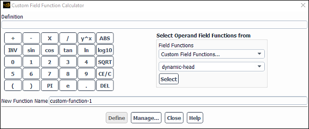
To create your own field function, you will use the Custom Field Function Calculator Dialog Box (Figure 42.3: The Custom Field Function Calculator Dialog Box). This dialog box allows you to define field functions based on existing functions, using simple calculator operators. Any functions that you define will be added to the list of default flow variables and other field functions provided by the solver.
![]() Parameters & Customization → Custom Field Functions
Parameters & Customization → Custom Field Functions
![]() New...
New...
Important: Recall that you must enter all constants in the function definition in SI units.
The steps for creating a custom field function are as follows:
Use the calculator buttons and the Field Functions list and Select button to specify the function definition, as described below. (As you select each item from the Field Functions list or click a button in the calculator keypad, its symbol will appear in the Definition text entry box. You cannot edit the contents of this box directly; if you want to delete part of a function, use the DEL button on the keypad.)
Important: The range of integers and real numbers that can be stored is as follows:


Note that using a number less than 1e-39 may produce inaccurate results, while values less than 1e-45 will produce a result of zero.
Specify the name of the function in the New Function Name field.
Important: Be sure that you do not specify a name that is already used for a standard field function (for example,
velocity-magnitude); you can see a complete list of the predefined field functions in Ansys Fluent by selecting thedisplay/contourstext command and viewing the available choices forcontours of.Click the Define button.
When you click Define, the solver will create the function and add it to the list of Custom Field Functions within the drop-down list of available field functions. The Define push button is grayed out after you create a new function or if the Definition text entry box is empty.
Should you decide to rename or delete the function after you have completed the definition, you can do so in the Field Function Definitions Dialog Box, which you can open by clicking on the Manage... push button. See Manipulating, Saving, and Loading Custom Field Functions for details.
Your function definition can include many basic calculator operations (for example, addition, subtraction, multiplication, square root). When you select a calculator button (by clicking on it), the appropriate symbol will appear in the Definition text entry box. The meaning of the buttons is straightforward; they are similar to the buttons you would find on any standard calculator. You should, however, note the following:
The CE/C button will clear the entire Definition and the New Function Name, if you have entered one. The DEL button will delete only the last entry in the Definition text entry box. You can use DEL to delete characters one at a time, starting with the last one entered.
To obtain the inverse trigonometric functions arcsin, arccos, and arctan, click the INV button before selecting sin, cos, or tan.
The ABS button yields the absolute value of the number that follows it. Likewise, the ln button yields the natural logarithm of the number that follows it, and the log10 button yields the base 10 logarithm function of the number that follows it.
Important: log10 and ln will be calculated for values greater than 0. For values less than or equal to 0, the resultant value will be zero.
The PI button represents
 and the e button represents the base of the natural logarithm system (which is
approximately equal to
and the e button represents the base of the natural logarithm system (which is
approximately equal to  ).
).
Your function definition can include any of the field functions defined by the solver (and listed in Alphabetical Listing of Field Variables and Their Definitions) or by you. You can also use any report definitions that you have created (see Monitoring and Reporting Solution Data for additional information). To include one of these variables/functions in your function definition, select it in the Field Functions drop-down list and then click the Select button below the list. The symbol for the selected item will appear in the Definition text entry box (for example, p will appear if you select Static Pressure).
Note: If a custom field function definition uses a report definition, then it cannot be exported to a file.
Once you have defined your field functions, you can manipulate them using the Field Function Definitions Dialog Box ( Figure 42.4: The Field Function Definitions Dialog Box). You can display a function definition to be sure that it is correct, delete the function if you decide that it is incorrect and must be redefined, or give the function a new name. You can also save custom field functions to a file or read them from a file. The custom field function file allows you to transfer your custom functions between case files.
To open the Field Function Definitions Dialog Box, right-click Custom Field Functions (under the Parameters & Customization branch of the tree) and select Manage.... You can also click the Manage... button in the Custom Field Function Calculator Dialog Box.
To open the Field Function Definitions Dialog Box, right-click Custom Field Functions (under the Parameters & Customization branch of the tree) and select Manage.... You can also click the Manage... button in the Custom Field Function Calculator Dialog Box.
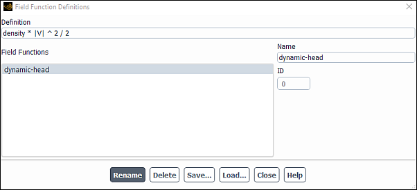
The following actions can be performed in the Field Function Definitions Dialog Box:
To check the definition of a function, select it in the Field Functions list. Its definition will be displayed in the Definition field. This display is for informational purposes only; you cannot edit it. If you want to change a function definition, you must delete the function and define it again in the Custom Field Function Calculator Dialog Box.
To delete a function, select it in the Field Functions list and click the Delete button.
To rename a function, select it in the Field Functions list, enter a new name in the Name field, and click the Rename button.
Important: Be sure that you do not specify a name that is already used for a standard field function (for example,
velocity-magnitude); you can see a complete list of the predefined field functions in Ansys Fluent by selecting thedisplay/contourstext command and viewing the available choices forcontours of.To save all of the functions in the Field Functions list to a file, click the Save... button and specify the file name in The Select File Dialog Box.
To read custom field functions from a file that you saved as described above, click the Load... button and specify the file name in the resulting Select File dialog box. (Custom field function files are valid Scheme functions, and can also be loaded with the File/Read/Scheme... ribbon tab item, as described in Reading Scheme Source Files.)
When you are checking the results of your simulation, you may find it useful to define some of the following field functions:
To define a function that determines the ratio of static pressure to inlet total pressure, use the relationship

(42–76)
where
 is the static pressure calculated by the solver,
  is the inlet total pressure, and
  is the operating pressure for the problem. Use the solver-defined function Static
Pressure for
is the operating pressure for the problem. Use the solver-defined function Static
Pressure for  , and the numerical value that you specified for Gauge Total Pressure in the Pressure Inlet Dialog Box for
  . Specify the value of the operating pressure to be the value that you set in the Operating Conditions Dialog Box. As discussed in Operating Pressure, all pressures in
Ansys Fluent are gauge pressures relative to the operating pressure. If the operating pressure is zero, as is generally the
case for compressible flow calculations, the expression for the pressure ratio reduces to
. Specify the value of the operating pressure to be the value that you set in the Operating Conditions Dialog Box. As discussed in Operating Pressure, all pressures in
Ansys Fluent are gauge pressures relative to the operating pressure. If the operating pressure is zero, as is generally the
case for compressible flow calculations, the expression for the pressure ratio reduces to
(42–77)
To define a function that determines the critical velocity ratio
 , a parameter that is sometimes used in turbomachinery calculations, use the relationship
(42–78)
In this relationship,
 is the critical velocity (that is, the velocity that would
occur for the same stagnation conditions if
is the critical velocity (that is, the velocity that would
occur for the same stagnation conditions if  ),
),  is the ratio of specific heats, and
  is the pressure ratio defined in Equation 42–77 for which you created your own
function. For
is the pressure ratio defined in Equation 42–77 for which you created your own
function. For  , ratio of specific heats, select Specific Heat
Ratio (gamma) in the Properties...
category. To include
, ratio of specific heats, select Specific Heat
Ratio (gamma) in the Properties...
category. To include  , select Custom Field Functions... in
the first drop-down list under Field Functions,
and then select from the second list the function name that you assigned
, select Custom Field Functions... in
the first drop-down list under Field Functions,
and then select from the second list the function name that you assigned
 .
.Suppose you have swirling flow in a pipe, aligned with the
 axis, and you want to calculate the flow rate of angular momentum through a cross-sectional plane:
(42–79)
You can create a function for the product
 , where
  is the Radial Coordinate and
  is the Tangential Velocity. Then use the Surface Integrals Dialog Box to
compute the flow rate of this quantity.
is the Tangential Velocity. Then use the Surface Integrals Dialog Box to
compute the flow rate of this quantity.
Important: The custom field function containing model dependent functions (like temperature when the energy equation is enabled) will be computed only when those models are still active.