


This section contains information about special geometry/mesh requirements and general comments on mesh quality.
You should be aware of the following geometry setup and mesh construction requirements at the beginning of your problem setup:
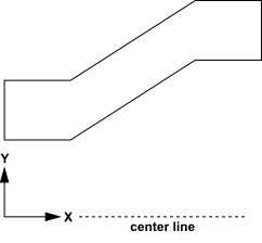
Axisymmetric geometries must be defined such that the axis of rotation is the
 axis of the Cartesian coordinates used to define the geometry (Figure 6.21: Setup of Axisymmetric Geometries with the x Axis as the Centerline).
 Ansys Fluent allows you to set up periodic boundaries using either conformal or non-conformal periodic zones. For conformal periodic boundaries, the periodic zones must have identical meshes.
The conformal periodic boundary zones can be created in the meshing mode of Fluent or GAMBIT when you are generating the volume mesh. See the Fluent Meshing section of the User’s Guide or the GAMBIT Modeling Guide for more information.
You can also use the solution mode of Fluent to create a periodic boundary zone pair from two conformal zones, as well as a periodic interface from non-conformal zones; the latter is necessary if you created your mesh using a CAD package that is not able to produce true periodic boundaries. For details on creating such interfaces, see Creating Periodic Zones and Interfaces.
The quality of the mesh plays a significant role in the accuracy and stability of the
numerical computation. Regardless of the type of mesh used in your domain, checking the
quality of your mesh is essential. One important indicator of mesh quality that
Ansys Fluent allows you to check is a quantity referred to as the orthogonality. In order
to determine the orthogonality of a given cell, the following quantities are calculated for
each face  :
:
the normalized dot product of the area vector of a face (
 ) and a vector from the centroid of the cell to the centroid of that
face (
) and a vector from the centroid of the cell to the centroid of that
face ( ):
):
(6–1)
the normalized dot product of the area vector of a face (
 ) and a vector from the centroid of the cell to the centroid of the
adjacent cell that shares that face (
) and a vector from the centroid of the cell to the centroid of the
adjacent cell that shares that face ( ):
):
(6–2)
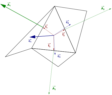
The minimum value that results from calculating Equation 6–1 and Equation 6–2 for all of the faces is then defined as the orthogonality for the cell. Therefore, the worst cells will have an orthogonality closer to 0 and the best cells will have an orthogonality closer to 1. Figure 6.22: The Vectors Used to Compute Orthogonality illustrates the relevant vectors.
This calculation of the orthogonality is used in (but is not always equal to) a metric referred to as the "orthogonal quality". By default, the orthogonal quality depends on the cell type:
For tetrahedral, prism, and pyramid cells, the orthogonal quality is the minimum of the orthogonality and (1- cell skewness).
For hexahedral and polyhedral cells, the orthogonal quality is the same as the orthogonality.
Note that you can use the following text command to specify that
the orthogonal quality uses an enhanced definition:
mesh/enhanced-orthogonal-quality?. When enabled, the orthogonal
quality is defined using a variety quality measures, including: the orthogonality of a face
relative to vectors from the cell centroid to the face centroid and to the neighboring cell
centroid; a metric that detects poor cell shape at a local edge (such as twisting and/or
concavity); and the variation of normals between the faces that can be constructed from the
cell face. This enhanced definition is optimal for evaluating thin prism cells.
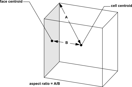
Another important indicator of the mesh quality is the aspect ratio. The aspect ratio is a measure of the stretching of a cell. It is computed as the ratio of the maximum value to the minimum value of any of the following distances: the normal distances between the cell centroid and face centroids (computed as a dot product of the distance vector and the face normal), and the distances between the cell centroid and nodes. For a unit cube (see Figure 6.23: Calculating the Aspect Ratio for a Unit Cube), the maximum distance is 0.866, and the minimum distance is 0.5, so the aspect ratio is 1.732. This type of definition can be applied on any type of mesh, including polyhedral.
To check the quality of your mesh, you can use the button in the General task page:
![]() Setup →
Setup → ![]() General
→ Report Quality
General
→ Report Quality
A message will be displayed in the console, such as the example that follows:
Mesh Quality:
 Orthogonal Quality ranges from 0 to 1, where values close to 0 correspond to low quality.
Minimum Orthogonal Quality = 6.07960e-01
Maximum Aspect Ratio = 5.42664e+00
If you would like more information about the quality displayed in the console (including
additional quality metrics and the zones that have the cells with the lowest quality), set
the mesh/check-verbosity text command to 2
(valid values are 0, 1,
2) prior to using the
button.
You can also get information about the number of cells and cell quality on a per cell zone basis. This can allow you to diagnose which cell zone contains poor quality cells.
![]() Setup → Cell Zone Conditions
→ <Zone Type>
Setup → Cell Zone Conditions
→ <Zone Type>
![]() Info
Info
You can also perform the same Info check on individual cell zones.
For information about how to improve poor quality cells, see Repairing Meshes. For information about avoiding divergence when cells with poor face orthogonality are near coupled two-sided walls, see Orthogonality-Based Secondary Gradient Limiting at Coupled Two-Sided Walls.
When evaluating whether the quality of your mesh is sufficient for the problem you are modeling, it is important to consider attributes such as mesh element distribution, cell shape, smoothness, and flow-field dependency. These attributes are described in the sections that follow.
Since you are discretely defining a continuous domain, the degree to which the salient features of the flow (such as shear layers, separated regions, shock waves, boundary layers, and mixing zones) are resolved depends on the density and distribution of mesh elements. In many cases, poor resolution in critical regions can dramatically affect results. For example, the prediction of separation due to an adverse pressure gradient depends heavily on the resolution of the boundary layer upstream of the point of separation.
Resolution of the boundary layer (that is, mesh spacing near walls) also plays a significant role in the accuracy of the computed wall shear stress and heat transfer coefficient. This is particularly true in laminar flows where the mesh adjacent to the wall should obey
 | (6–3) |
| where | |
|
| |
|
| |
|
| |
|
|


Equation 6–3 is based upon the Blasius solution for laminar flow over a flat plate at zero incidence [137].
Proper resolution of the mesh for turbulent flows is also very important. Due to the strong interaction of the mean flow and turbulence, the numerical results for turbulent flows tend to be more susceptible to mesh element distribution than those for laminar flows. In the near-wall region, different mesh resolutions are required depending on the near-wall model being used. See Model Hierarchy for guidelines.
In general, no flow passage should be represented by fewer than 5 cells. Most cases will require many more cells to adequately resolve the passage. In regions of large gradients, as in shear layers or mixing zones, the mesh should be fine enough to minimize the change in the flow variables from cell to cell. Unfortunately, it is very difficult to determine the locations of important flow features in advance. Moreover, the mesh resolution in most complicated 3D flow fields will be constrained by CPU time and computer resource limitations (that is, memory and disk space). Although accuracy increases with larger meshes, the CPU and memory requirements to compute the solution and postprocess the results also increase. Solution-adaptive mesh refinement can be used to increase and/or decrease mesh density based on the evolving flow field, and therefore provides the potential for more economical use of grid points (and hence reduced time and resource requirements). See Adapting the Mesh for information on solution adaption.
The quality of the cell (including its orthogonal quality, aspect ratio, and skewness) also has a significant impact on the accuracy of the numerical solution.
Orthogonal quality is computed as described in Mesh Quality. The worst cells will have an orthogonal quality closer to 0, with the best cells closer to 1. The minimum orthogonal quality for all types of cells should be more than 0.01, with an average value that is significantly higher.
Aspect ratio is a measure of the stretching of the cell. As discussed in Computational Expense, for highly anisotropic flows, extreme aspect ratios may yield accurate results with fewer cells. Generally, it is best to avoid sudden and large changes in cell aspect ratios in areas where the flow field exhibit large changes or strong gradients.
Skewness is defined as the difference between the shape of the cell and the shape of an equilateral cell of equivalent volume. Highly skewed cells can decrease accuracy and destabilize the solution. For example, optimal quadrilateral meshes will have vertex angles close to 90 degrees, while triangular meshes should preferably have angles of close to 60 degrees and have all angles less than 90 degrees. A general rule is that the maximum skewness for a triangular/tetrahedral mesh in most flows should be kept below 0.95, with an average value that is significantly lower. A maximum value above 0.95 may lead to convergence difficulties and may require changing the solver controls, such as reducing under-relaxation factors and/or switching to the pressure-based coupled solver.
Cell size change and face warp are additional quality measure that could affect stability and accuracy. See the Fluent Meshing section of the User’s Guide for more details.
Truncation error is the difference between the partial derivatives in the governing equations and their discrete approximations. Rapid changes in cell volume between adjacent cells translate into larger truncation errors. Ansys Fluent provides the capability to improve the smoothness by refining the mesh based on the change in cell volume or the gradient of cell volume. For information on marking cells by cell volume and then refining the mesh, see Volume and Refining and Coarsening.
The effect of resolution, smoothness, and cell shape on the accuracy and stability of the solution process is dependent on the flow field being simulated. For example, very skewed cells can be tolerated in benign flow regions, but can be very damaging in regions with strong flow gradients.
Since the locations of strong flow gradients generally cannot be determined a priori, you should strive to achieve a high-quality mesh over the entire flow domain.