


When a particle reaches a physical boundary (for example, a wall or inlet boundary) in your model, Ansys Fluent applies a discrete phase boundary condition to determine the fate of the trajectory at that boundary. One of several contingencies may arise:
The particle may be reflected via an elastic or inelastic collision.
The particle may escape through the boundary. The particle is lost from the calculation at the point where it impacts the boundary.
The particle may be trapped at the wall. Nonvolatile material is lost from the calculation at the point of impact with the boundary; volatile material present in the particle or droplet is released to the vapor phase at this point.
The particle may pass through an internal boundary zone, such as radiator or porous jump.
The particle may slide along the wall, depending on particle properties and impact angle.
The particle may form a film (wall film model).
The particle may be reinjected using location and particle velocity information from a specified injection.
You also have the option of implementing a user-defined function to model the particle behavior when hitting the boundary. More information about user-defined functions can be found in the Fluent Customization Manual.
The boundary condition, or trajectory fate, can be defined separately for each zone in your Ansys Fluent model.
For additional information, see the following sections:
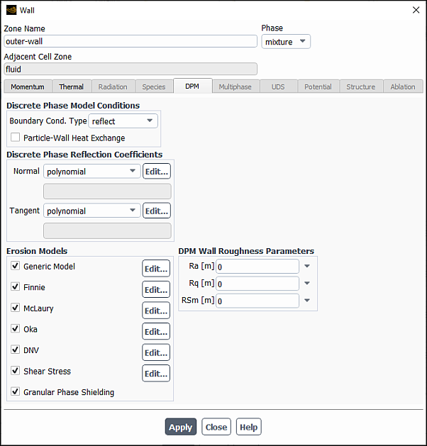
Discrete phase boundary conditions can be set for boundaries in the dialog boxes opened from the Boundary Conditions task page. When one or more injections have been defined, inputs for the discrete phase will appear in the dialog boxes. In the Walls dialog boxes, you will need to click the DPM tab to access the Discrete Phase Model Boundary Conditions as shown in Figure 24.39: Discrete Phase Boundary Conditions in the Wall Dialog Box.
The available boundary conditions are:
reflect
trap
escape
wall-jet
wall-film
interior
user-defined
Because you can stipulate any of these conditions at flow boundaries, it is possible to incorporate mixed discrete phase boundary conditions in your Ansys Fluent model.
Further details are discussed in the following sections:
- 24.4.1.1. The reflect Boundary Condition
- 24.4.1.2. The trap Boundary Condition
- 24.4.1.3. The escape Boundary Condition
- 24.4.1.4. The wall-jet Boundary Condition
- 24.4.1.5. The wall-film Boundary Condition
- 24.4.1.6. The interior Boundary Condition
- 24.4.1.7. The reinject Boundary Condition
- 24.4.1.8. The user-defined Boundary Condition
The particle rebounds off the boundary with a change in its momentum. Ansys Fluent provides two models for computing this change:
For non-rotating particles, the momentum depends on the coefficient of restitution (Equation 12–193 in the Fluent Theory Guide).
For rotating particles, the model proposed by Tsuji et al. 660 is used. The particle rotation model includes frictional effects.
The details on these two models can be found in Wall-Particle Reflection Model Theory in the Fluent Theory Guide.
For information on how to set up the parameters for non-rotating and rotating particle models, see Coefficients of Restitution and Friction Coefficient, respectively.
When at least one injection accounts for the rough wall model (the Rough Wall Model option is selected under the Physical Models tab in the Set Injections Properties dialog box), you can specify the wall surface roughness parameters as described in Rough Wall Model.
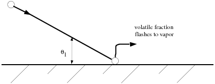
The trajectory calculations are terminated and the fate of the particle is recorded as “trapped”. In the case of evaporating droplets, their entire mass instantaneously passes into the vapor phase and enters the cell adjacent to the boundary. See Figure 24.40: “Trap” Boundary Condition for the Discrete Phase. In the case of combusting particles, the remaining volatile mass is passed into the vapor phase. No further char combustion occurs. The particle no longer participates in heat transfer.
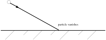
The particle is reported as having “escaped” when it encounters the boundary in question. Trajectory calculations are terminated. See Figure 24.41: “Escape” Boundary Condition for the Discrete Phase.
The wall-jet type boundary condition is appropriate for high-temperature walls where no significant liquid film is formed, and in high-Weber-number impacts where the spray acts as a jet. The model is not appropriate for regimes where film is important (for example, port fuel injection in SI engines, rainwater runoff, and so on).
A more detailed description of underlying theory is available in Wall-Jet Model Theory in the Theory Guide.
The wall-film boundary condition is used for modeling Lagrangian wall films. See Setting the Lagrangian Wall Film Model for a detailed description of the functionality and options available.
The interior boundary condition means that the particles will pass through the internal boundary. This option is available only for internal boundary zones, such as a radiator or a porous jump.
The reinject boundary condition reintroduces DPM particles into the domain when they reach a certain domain boundary (for example, outlet). The location and velocity at which such recirculated particles are reinjected is taken from a user-specified injection, while all other particle properties remain unchanged.
As an application example, the reinject boundary condition type can be useful in simulating a fluidized bed, where usually the details of the external piping and gas-solid separators are not resolved in the computational mesh. In such cases, the reinject boundary condition can be used to model the reintroduction of the particles that have left the reactor vessel.
To use this boundary condition:
In the Boundary Conditions task page, select the zone to which you want to assign the reinject boundary condition and click Edit….
In the DPM tab of the corresponding boundary condition dialog box that opens, select reinject from the Discrete Phase BC Type drop-down list.
In the Use Settings From drop-down list, select an injection whose properties will be used for reintroducing particles back to the domain.
The settings of the selected injection are used to assign every particle that reaches the boundary a new position and new velocity.
You can either use an existing injection that is also used for injecting new particles or create a separate injection only for specifying a location and initial velocity of reinjected particles. In the latter case, select Reinjection Only in the Set Injection Properties dialog box (Particle Reinjection group box) for that injection, so that it never introduces any particles by itself. Like the particle reinjection option, this option is available only when unsteady particle tracking is enabled.
Note: For postprocessing and reporting, a reinjected particle remains associated with the injection from which it was originally injected.
If particles require a significant period of time when they are transported from the outlet to the location of reinjection, you can delay the reinjection by a specified amount of time as follows:
In the Set Injection Properties dialog box, make sure that Reinjection Only is selected for the injection.
In the Point Properties tab, specify Reinjection Time Delay.
Particles that are delayed during reinjection will immediately appear at the new location in graphical postprocessing, but they will not move or participate in any interaction with the continuous phase until their individual delay period has passed.
Interpreting DPM Summary Reports in conjunction with particle reinjection is described in Reinjected Particles
You can use a DEFINE_DPM_BC user-defined function (UDF) to modify
the behavior of particle reinjection as shown in Example 5 in the Fluent Customization Manual.
It is also possible to use a user-defined function to compute the behavior of the particles at a physical boundary. More information about user-defined functions can be found in the Fluent Customization Manual.
Ansys Fluent makes the following assumptions regarding boundary conditions:
The reflect type is assumed at wall, symmetry, and axis boundaries, with both coefficients of restitution equal to 1.0
The escape type is assumed at all flow boundaries (pressure and velocity inlets, pressure outlets, and so on)
The interior type is assumed at all internal boundaries (radiator, porous jump, and so on)
The coefficient of restitution can be modified only for wall boundaries.
A normal or tangential coefficient of restitution equal to 1.0 implies that the particle retains all of its normal or tangential momentum after the rebound (an elastic collision). A normal or tangential coefficient of restitution equal to 0.0 implies that the particle retains none of its normal or tangential momentum after the rebound.
Nonconstant coefficients of restitution can be specified for wall zones with the
reflect type boundary condition. The coefficients are set as a function of
the impact angle,  , in Particle Reflection at Wall in the Fluent Theory Guide.
Note that the default setting for both coefficients of restitution is a constant value of 1.0 (all normal and tangential momentum retained).
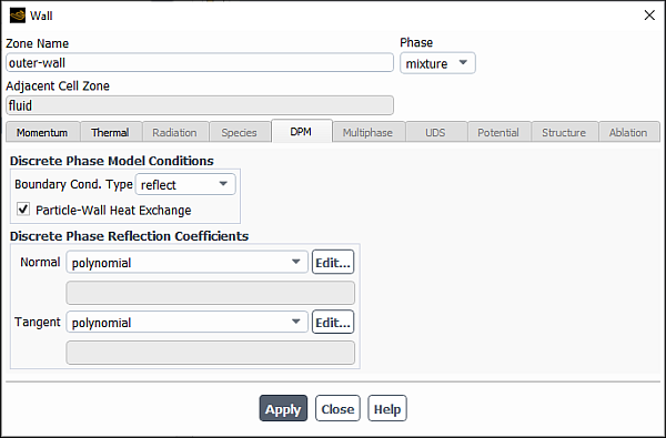
If you select the reflect type at a wall (only), you can define the Normal and Tangent coefficients of restitution under Discrete Phase Reflection Coefficients. You can select a constant, polynomial, piecewise-linear, or piecewise-polynomial function from the relevant drop-down lists. The dialog boxes for defining the polynomial, piecewise-linear, and piecewise-polynomial functions are the same as those used for defining temperature-dependent properties. The applied wall heat transfer model assumes that a liquid is getting in contact with the wall. See Defining Properties Using Temperature-Dependent Functions for details.
When at least one injection accounts for particle rotation (the Enable Rotation option is selected under the Physical Models tab in the Set Injections Properties dialog box), you can specify friction coefficients for wall zones with the reflect type boundary condition. In the Wall dialog box, under the DPM tab, you can define the Friction Coefficient as a constant or as a polynomial, piecewise-linear, or piecewise-polynomial function.
The default value for the constant is 0.2. For the piecewise-linear and piecewise-polynomial profiles, the friction coefficient is computed in terms of the relative tangential velocity. The default inputs for these functions are derived from the friction collision law (The Friction Collision Law in the Fluent Theory Guide) and are as follows.
The piecewise-linear approximation is defined using the following default points for the relative (particle-to-wall) tangential velocity:
Point 1: 0 m/s
Point 2: 1 m/s
Point 3: 10 m/s
Point 4: 210 m/s
The piecewise-polynomial approximation is defined in the three relative (particle-to-wall) tangential velocity ranges as follows:
Range 1: 0–1 m/s: a quadratic function
Range 2: 1–10 m/s: a constant
Range 3: 10–210 m/s: a linear function
For details about using the Piecewise-Linear Profile dialog box and Piecewise-Polynomial Profile dialog box see Inputs for Piecewise-Linear Functions and Inputs for Piecewise-Polynomial Functions, respectively.
To enable the particle-to-wall heat exchange for the reflect, wall-jet, or wall-film boundary conditions: In the Wall dialog box, under the DPM tab, enable the Particle-Wall Heat Exchange option. The option is available only for wall boundary conditions and unsteady particle tracking when the energy equation is enabled.
Note that when a particle is reflected from a wall with the wall film DPM boundary condition, the particle-to-wall heat exchange is calculated directly between the particle and the wall. Any wall film present is not taken into account.
The model is applied for all inert, droplet, and multicomponent particles impinging on the wall. The specific model is not applied for the splashed particles. When the wall film DPM boundary condition is active, the model is applied in the Rebound Regime, and it is assumed that the particles hit the wall irrespective of the presence of a film. In the Splashing regime, the mass fraction that is deposited mixes with any existing film, and the splashed particles retain the impinging droplet temperature.
For combusting particles, the wall heat transfer is calculated only if the Wet Combustion Model option is enabled in the Set Injection Properties dialog box, and the particle liquid fraction is nonzero, otherwise the Particle-Wall Heat Exchange option has no effect.
See Particle–Wall Impingement Heat Transfer Theory in the Fluent Theory Guide for the underlying theory and equations of the particle–wall impingement heat transfer model.
If the Erosion/Accretion option is selected in the Physical Models tab of the Discrete Phase Model Dialog Box (see Monitoring Erosion/Accretion of Particles at Walls), you can enable erosion models in the DPM tab of the Wall Dialog Box and specify the corresponding erosion rate parameters at the walls. Note that if you are setting up erosion / accretion between a fluid and solid zone, the erosion models must be enabled on the fluid side of the coupled wall.
Important: The default erosion rate parameters for each erosion model may not be appropriate for your analysis and must be adjusted based on your own experimental data.
The following models are available in Ansys Fluent:
Generic Model
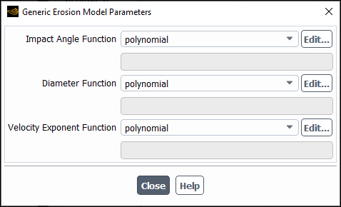
The erosion rate of the generic model is defined in Equation 12–346 in the Theory Guide as a product of the mass flux and specified functions for the particle diameter, impact angle, and velocity exponent. To specify the erosion parameters for the Generic model, click Edit... next to Generic Model.
In the Generic Erosion Model Parameters dialog box, specify the following parameters using a constant, polynomial, piecewise-linear, or piecewise-polynomial function:
Impact Angle Function:
 in Equation 12–346 in the Fluent Theory Guide.
Diameter Function:
 in Equation 12–346 in the Fluent Theory Guide.
Velocity Exponent Function:
 in Equation 12–346 in the Fluent Theory Guide.
See Accretion in the Theory Guide for a detailed description of these functions and Defining Properties Using Temperature-Dependent Functions for details about using the dialog boxes for defining polynomial, piecewise-linear, and piecewise-polynomial functions.
Finnie
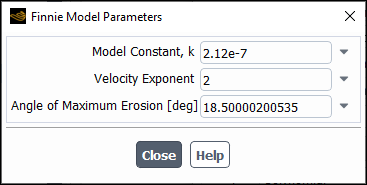
To specify the erosion parameters for the Finnie model, click Edit... next to Finnie.
In the Finnie Model Parameters dialog box, specify the following parameters:
Model Constant, k:
 in Equation 12–331 in the Fluent Theory Guide.
Velocity Exponent:
 in Equation 12–331 in the Fluent Theory Guide. The default value is 2. The value of the Velocity Exponent is generally within the range of 2.3 to 2.5 for metals.
Angle of Maximum Erosion: the impact angle between the approaching particle track and the wall at which the erosion reaches maximum.
For information about the theory behind the Finnie model, see Finnie Erosion Model in the Fluent Theory Guide.
McLaury
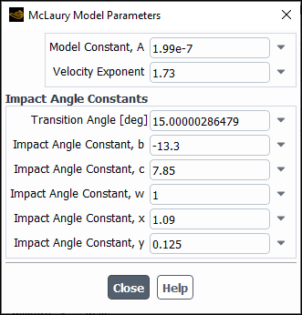
To specify the erosion parameters for the McLaury model, click Edit... next to McLaury.
In the McLaury Model Parameters dialog box, specify the following parameters:
Model Constant, A:
 in Equation 12–335 in the Fluent Theory Guide.
Velocity Exponent:
 in Equation 12–335 in the Fluent Theory Guide.
Transition Angle:
 in Equation 12–336 and Equation 12–337 in the Fluent Theory Guide.
Impact Angle Constant, b:
 in Equation 12–336 in the Fluent Theory Guide.
Impact Angle Constant, c:
 in Equation 12–336 in the Fluent Theory Guide.
Impact Angle Constant, w:
 in Equation 12–337 in the Fluent Theory Guide.
Impact Angle Constant, x:
 in Equation 12–337 in the Fluent Theory Guide.
Impact Angle Constant, y:
 in Equation 12–337 in the Fluent Theory Guide.
See Example of the McLaury Erosion Model Constants in the Fluent Theory Guide for more information about the McLaury model parameters. For theoretical background on the McLaury model, see McLaury Erosion Model in the Fluent Theory Guide.
Oka
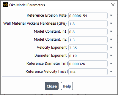
To specify the erosion parameters for the Oka model, click Edit... next to Oka.
In the Oka Model Parameters dialog box, specify the following parameters:
Reference Erosion Rate:
 in Equation 12–333 in the Fluent Theory Guide.
Wall Material Hardness:
 in Equation 12–334 in the Fluent Theory Guide.
Model Constant, n1:
 in Equation 12–334 in the Fluent Theory Guide.
Model Constant, n2:
 in Equation 12–334 in the Fluent Theory Guide.
Velocity Exponent:
 in Equation 12–333 in the Fluent Theory Guide.
Diameter Exponent:
 in Equation 12–333 in the Fluent Theory Guide.
Reference Diameter:
 in Equation 12–333 in the Fluent Theory Guide.
Reference Velocity:
 in Equation 12–333 in the Fluent Theory Guide.
See Example of the Oka Erosion Model Constants in the Fluent Theory Guide for an example of the Oka model parameters' values. For more information on the theory behind the Oka model, see Oka Erosion Model in the Fluent Theory Guide.
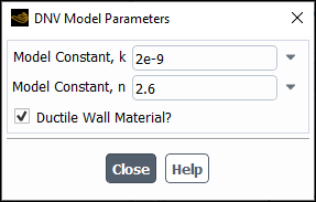
DNV
To specify the erosion parameters for the DNV model, click Edit... next to DNV.
In the DNV Model Parameters dialog box, specify the following parameters:
Model Constant, k:
 in Equation 12–338 in the Fluent Theory Guide.
Model Constant, n:
 in Equation 12–338 in the Fluent Theory Guide.
Ductile Wall Material?: When enabled, specifies that the wall material is ductile.
For information about the theory behind the DNV model, see DNV Erosion Model in the Fluent Theory Guide.
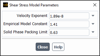
Shear Stress (dense flows with the disperse granular phase only)
To specify the erosion parameters for the shear stress model, click Edit... next to Shear Stress.
In the Shear Stress Model Parameters dialog box, specify the following parameters:
Velocity Exponent:
 in Equation 12–341 in the Fluent Theory Guide.
Empirical Model Constant:
 in Equation 12–341 in the Fluent Theory Guide.
Solid Phase Packing Limit:
 in Equation 12–341 in the Fluent Theory Guide.
This model should be used for dense multiphase flow with a dispersed phase consisting of solid particles. For more information on the theory behind the shear stress model, see Abrasive Erosion Caused by Solid Particles in the Fluent Theory Guide.
Granular Phase Shielding (dense flows with the disperse granular phase only)
The granular phase shielding as given by Equation 12–344 in the Fluent Theory Guide is always considered in the shear stress erosion model. If you want to include the shielding effect in other erosion models that are currently enabled, select Granular Phase Shielding. This option is available only when Shear Stress Model Parameters is selected.
For more information about the theory behind the wall shielding effects in dense flows, see Wall Shielding Effect in Dense Flow Regimes in the Fluent Theory Guide.
By default, all erosion models are enabled.
Important:
The default constants for the Finnie, Oka, and McLaury models have been tuned to match the experiment described by Oka [108] in which 326-micron sand particles impact a carbon steel wall at a speed of 104 m/s and therefore are only valid for those specific conditions. You can use the default values as a starting point for your simulation and then adjust them as needed.
Predictive capabilities of the erosion models are limited and strongly case dependent.