As discussed in The Multiple Reference Frame Model, the MRF model is applicable when the flow at the interface between adjacent moving/stationary zones is nearly uniform (“mixed out”). If the flow at this interface is not uniform, the MRF model may not provide a physically meaningful solution. The sliding mesh model (see Modeling Flows Using Sliding and Dynamic Meshes in the User's Guide) may be appropriate for such cases, but in many situations it is not practical to employ a sliding mesh. For example, in a multistage turbomachine, if the number of blades is different for each blade row, a large number of blade passages is required in order to maintain circumferential periodicity. Moreover, sliding mesh calculations are necessarily unsteady, and therefore require significantly more computation to achieve a final, time-periodic solution. For situations where using the sliding mesh model is not feasible, the mixing plane model can be a cost-effective alternative.

In the mixing plane approach, each fluid zone is treated as a steady-state problem. Flow-field data from adjacent zones are passed as boundary conditions that are spatially averaged or “mixed” at the mixing plane interface. This mixing removes any unsteadiness that would arise due to circumferential variations in the passage-to-passage flow field (for example, wakes, shock waves, separated flow), therefore yielding a steady-state result. Despite the simplifications inherent in the mixing plane model, the resulting solutions can provide reasonable approximations of the time-averaged flow field.

Consider the turbomachine stages shown schematically in Figure 2.7: Axial Rotor-Stator Interaction (Schematic Illustrating the Mixing Plane Concept) and Figure 2.8: Radial Rotor-Stator Interaction (Schematic Illustrating the Mixing Plane Concept), each blade passage contains periodic boundaries. Figure 2.7: Axial Rotor-Stator Interaction (Schematic Illustrating the Mixing Plane Concept) shows a constant radial plane within a single stage of an axial machine, while Figure 2.8: Radial Rotor-Stator Interaction (Schematic Illustrating the Mixing Plane Concept) shows a constant plane within a mixed-flow device. In each case, the stage consists of two flow domains: the rotor domain, which is rotating at a prescribed angular velocity, followed by the stator domain, which is stationary. The order of the rotor and stator is arbitrary (that is, a situation where the rotor is downstream of the stator is equally valid).

Figure 2.7: Axial Rotor-Stator Interaction (Schematic Illustrating the Mixing Plane Concept)

Figure 2.8: Radial Rotor-Stator Interaction (Schematic Illustrating the Mixing Plane Concept)

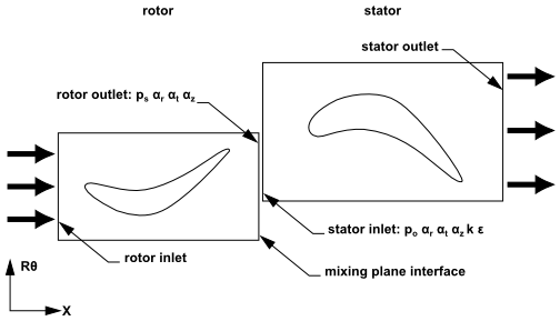
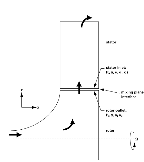
In a numerical simulation, each domain will be represented by a separate mesh. The flow information between these domains will be coupled at the mixing plane interface (as shown in Figure 2.7: Axial Rotor-Stator Interaction (Schematic Illustrating the Mixing Plane Concept) and Figure 2.8: Radial Rotor-Stator Interaction (Schematic Illustrating the Mixing Plane Concept)) using the mixing plane model. Note that you may couple any number of fluid zones in this manner; for example, four blade passages can be coupled using three mixing planes.

The essential idea behind the mixing plane concept is that each fluid zone is solved as a steady-state problem. At some prescribed iteration interval, the flow data at the mixing plane interface are averaged in the circumferential direction on both the stator outlet and the rotor inlet boundaries. The Ansys Fluent implementation gives you the choice of three types of averaging methods: area-weighted averaging, mass averaging, and mixed-out averaging. By performing circumferential averages at specified radial or axial stations, “profiles” of boundary condition flow variables can be defined. These profiles—which will be functions of either the axial or the radial coordinate, depending on the orientation of the mixing plane—are then used to update boundary conditions along the two zones of the mixing plane interface. In the examples shown in Figure 2.7: Axial Rotor-Stator Interaction (Schematic Illustrating the Mixing Plane Concept) and Figure 2.8: Radial Rotor-Stator Interaction (Schematic Illustrating the Mixing Plane Concept), profiles of averaged total pressure (), direction cosines of the local flow angles in the radial, tangential, and axial directions (), total temperature (), turbulence kinetic energy (), and turbulence dissipation rate () are computed at the rotor exit and used to update boundary conditions at the stator inlet. Likewise, a profile of static pressure (), direction cosines of the local flow angles in the radial, tangential, and axial directions (), are computed at the stator inlet and used as a boundary condition on the rotor exit.

Passing profiles in the manner described above assumes specific boundary condition types have been defined at the mixing plane interface. The coupling of an upstream outlet boundary zone with a downstream inlet boundary zone is called a “mixing plane pair”. In order to create mixing plane pairs in Ansys Fluent, the boundary zones must be of the following types:

For specific instructions about setting up mixing planes, see Setting Up the Legacy Mixing Plane Model in the User's Guide.

Three profile averaging methods are available in the mixing plane model:

 

2.3.2.4.1. Area Averaging

Area averaging is the default averaging method and is given by

(2–17)

---

Important:  The pressure and temperature obtained by the area average may not be representative of the momentum and energy of the flow.

---

 

2.3.2.4.2. Mass Averaging

Mass averaging is given by

(2–18)

where

(2–19)

This method provides a better representation of the total quantities than the area-averaging method. Convergence problems could arise if severe reverse flow is present at the mixing plane. Therefore, for solution stability purposes, it is best if you initiate the solution with area averaging, then switch to mass averaging after reverse flow dies out.

---

Important:  Mass averaging is not available with multiphase flows.

---

 

2.3.2.4.3. Mixed-Out Averaging

The mixed-out averaging method is derived from the conservation of mass, momentum and energy:

(2–20)

Because it is based on the principles of conservation, the mixed-out average is considered a better representation of the flow since it reflects losses associated with non-uniformities in the flow profiles. However, like the mass-averaging method, convergence difficulties can arise when severe reverse flow is present across the mixing plane. Therefore, it is best if you initiate the solution with area averaging, then switch to mixed-out averaging after reverse flow dies out.

Mixed-out averaging assumes that the fluid is a compressible ideal-gas with constant specific heat, .

---

Important:  Mixed-out averaging is not available with multiphase flows.

---

Ansys Fluent’s basic mixing plane algorithm can be described as follows:

Note that the algorithm described above will not rigorously conserve mass flow across the mixing plane if it is represented by a pressure outlet and pressure inlet mixing plane pair. If you use a pressure outlet and mass-flow inlet pair instead, Ansys Fluent will force mass conservation across the mixing plane. The basic technique consists of computing the mass flow rate across the upstream zone (pressure outlet) and adjusting the mass flux profile applied at the mass-flow inlet such that the downstream mass flow matches the upstream mass flow. This adjustment occurs at every iteration, therefore ensuring rigorous conservation of mass flow throughout the course of the calculation.

By default, Ansys Fluent does not conserve swirl across the mixing plane. For applications such as torque converters, where the sum of the torques acting on the components should be zero, enforcing swirl conservation across the mixing plane is essential, and is available in Ansys Fluent as a modeling option. Ensuring conservation of swirl is important because, otherwise, sources or sinks of tangential momentum will be present at the mixing plane interface.

Consider a control volume containing a stationary or moving component (for example, a pump impeller or turbine vane). Using the moment of momentum equation from fluid mechanics, it can be shown that for steady flow,

(2–21)

where is the torque of the fluid acting on the component, is the radial distance from the axis of rotation, is the absolute tangential velocity, is the total absolute velocity, and is the boundary surface. (The product is referred to as swirl.)

For a circumferentially periodic domain, with well-defined inlet and outlet boundaries, Equation 2–21 becomes

(2–22)

where inlet and outlet denote the inlet and outlet boundary surfaces.

Now consider the mixing plane interface to have a finite streamwise thickness. Applying Equation 2–22 to this zone and noting that, in the limit as the thickness shrinks to zero, the torque should vanish, the equation becomes

(2–23)

where upstream and downstream denote the upstream and downstream sides of the mixing plane interface. Note that Equation 2–23 applies to the full area (360 degrees) at the mixing plane interface.

Equation 2–23 provides a rational means of determining the tangential velocity component. That is, Ansys Fluent computes a profile of tangential velocity and then uniformly adjusts the profile such that the swirl integral is satisfied. Note that interpolating the tangential (and radial) velocity component profiles at the mixing plane does not affect mass conservation because these velocity components are orthogonal to the face-normal velocity used in computing the mass flux.

By default, Ansys Fluent does not conserve total enthalpy across the mixing plane. For some applications, total enthalpy conservation across the mixing plane is very desirable, because global parameters such as efficiency are directly related to the change in total enthalpy across a blade row or stage. This is available in Ansys Fluent as a modeling option.

The procedure for ensuring conservation of total enthalpy simply involves adjusting the downstream total temperature profile such that the integrated total enthalpy matches the upstream integrated total enthalpy. For multiphase flows, conservation of mass, swirl, and enthalpy are calculated for each phase. However, for the Eulerian multiphase model, since mass-flow inlets are not permissible, conservation of the above quantities does not occur.