


The main assumption of the DTRM is that the radiation leaving the surface element in a certain range of solid angles can be approximated by a single ray. This section provides details about the equations used in the DTRM. For information about setting up the model, see Setting Up the DTRM in the User's Guide.
The equation for the change of radiant intensity,  , along a
path,
, along a
path,  , can be written as
 | (5–57) |
|
where | |
|
| |
|
| |
|
| |
|
|


Here, the refractive index is assumed to be unity. The DTRM
integrates Equation 5–57 along a series of rays
emanating from boundary faces. If  is constant along the ray, then
  can be
estimated as
can be
estimated as
 | (5–58) |
where  is the radiant
intensity at the start of the incremental path, which is determined
by the appropriate boundary condition (see the description of boundary
conditions, below). The energy source in the fluid due to radiation
is then computed by summing the change in intensity along the path
of each ray that is traced through the fluid control volume.
is the radiant
intensity at the start of the incremental path, which is determined
by the appropriate boundary condition (see the description of boundary
conditions, below). The energy source in the fluid due to radiation
is then computed by summing the change in intensity along the path
of each ray that is traced through the fluid control volume.
The "ray tracing" technique used in the DTRM can provide a prediction of radiative heat transfer between surfaces without explicit view factor calculations. The accuracy of the model is limited mainly by the number of rays traced and the computational mesh.
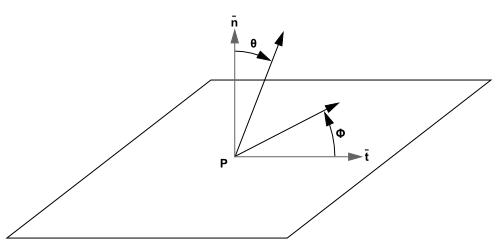
The ray paths are calculated and stored prior to the fluid flow
calculation. At each radiating face, rays are fired at discrete values
of the polar and azimuthal angles (see Figure 5.2: Angles θ and φ Defining the Hemispherical Solid Angle
About a Point P). To cover the radiating hemisphere,
 is varied from
  to
to  and
and  from
from  to
to  . Each ray
is then traced to determine the control volumes it intercepts as well
as its length within each control volume. This information is then
stored in the radiation file, which must be read in before the fluid
flow calculations begin.
. Each ray
is then traced to determine the control volumes it intercepts as well
as its length within each control volume. This information is then
stored in the radiation file, which must be read in before the fluid
flow calculations begin.
DTRM is computationally very expensive when there are too many surfaces to trace rays from and too many volumes crossed by the rays. To reduce the computational time, the number of radiating surfaces and absorbing cells is reduced by clustering surfaces and cells into surface and volume "clusters". The volume clusters are formed by starting from a cell and simply adding its neighbors and their neighbors until a specified number of cells per volume cluster is collected. Similarly, surface clusters are made by starting from a face and adding its neighbors and their neighbors until a specified number of faces per surface cluster is collected.
The incident radiation flux,  ,
and the volume sources are calculated for the surface and volume clusters
respectively. These values are then distributed to the faces and cells
in the clusters to calculate the wall and cell temperatures. Since
the radiation source terms are highly nonlinear (proportional to the
fourth power of temperature), care must be taken to calculate the
average temperatures of surface and volume clusters and distribute
the flux and source terms appropriately among the faces and cells
forming the clusters.
,
and the volume sources are calculated for the surface and volume clusters
respectively. These values are then distributed to the faces and cells
in the clusters to calculate the wall and cell temperatures. Since
the radiation source terms are highly nonlinear (proportional to the
fourth power of temperature), care must be taken to calculate the
average temperatures of surface and volume clusters and distribute
the flux and source terms appropriately among the faces and cells
forming the clusters.
The surface and volume cluster temperatures are obtained by area and volume averaging as shown in the following equations:
 | (5–59) |
 | (5–60) |
where  and
and  are the temperatures of the
surface and volume clusters respectively,
are the temperatures of the
surface and volume clusters respectively,  and
and  are the area
and temperature of face
are the area
and temperature of face  , and
, and  and
and  are the volume
and temperature of cell
are the volume
and temperature of cell  . The summations are carried over all faces of a
surface cluster and all cells of a volume cluster.
. The summations are carried over all faces of a
surface cluster and all cells of a volume cluster.
The radiation intensity approaching a point on a wall surface
is integrated to yield the incident radiative heat flux,  , as
, as
 | (5–61) |
where  is the hemispherical solid angle,
  is the intensity of the incoming ray,
  is the ray direction vector, and
  is the normal
pointing out of the domain. The net radiative heat flux from the surface,
is the normal
pointing out of the domain. The net radiative heat flux from the surface,  , is then computed as a sum of the reflected portion
of
, is then computed as a sum of the reflected portion
of  and the emissive
power of the surface:
and the emissive
power of the surface:
 | (5–62) |
where  is the surface temperature
of the point
is the surface temperature
of the point  on the surface and
  is the wall
emissivity which you enter as a boundary condition. Ansys Fluent incorporates
the radiative heat flux (Equation 5–62) in the
prediction of the wall surface temperature. Equation 5–62 also provides the surface boundary condition
for the radiation intensity
is the wall
emissivity which you enter as a boundary condition. Ansys Fluent incorporates
the radiative heat flux (Equation 5–62) in the
prediction of the wall surface temperature. Equation 5–62 also provides the surface boundary condition
for the radiation intensity  of a ray emanating
from the point
of a ray emanating
from the point  , as
, as
 | (5–63) |
The net radiative heat flux at flow inlets and outlets is computed in the same manner as at walls, as described above. Ansys Fluent assumes that the emissivity of all flow inlets and outlets is 1.0 (black body absorption) unless you choose to redefine this boundary treatment.
Ansys Fluent includes an option that allows you to use different temperatures for radiation and convection at inlets and outlets. This can be useful when the temperature outside the inlet or outlet differs considerably from the temperature in the enclosure. For details, see Defining Boundary Conditions for Radiation in the User's Guide.