6.8. Controlling Flow in Narrow Gaps for Valves and Pumps

When using dynamic meshes, overset meshes, and/or sliding meshes to simulate flow through narrow gaps that open or close over time (such as in a valve or a rotary pump), you can use the gap model to block or decelerate the flow when the gaps are closed. The following sections provide details:

6.8.1. The Gap Model Approach

For transient flows with moving face zones, narrow gaps may open or close during every time step. You can use the gap model to simulate the blockage of flow when a gap is closed. A gap region is made up of a pair of face zones, so that when one moves within a specified proximity threshold distance of the other, the fluid cells within the threshold of the zones are marked, and then the flow is blocked at the boundary faces of the marked region so that the marked cells no longer participate in the solution (for what is called a flow-blocking type region) or else decelerated in the marked region (for what is called a flow-modeling type region). The gap model has the following advantages:

With the flow-blocking type, you can ensure that there is no flow leakage. This is a realistic flow condition for valves in the closed position.
When the flow-blocking type does not produce a stable solution or is otherwise not preferred, you can use the flow-modeling type to decelerate the flow inside the gap regions and minimize leakage.
It can reduce computational cost in narrow gaps by reducing the need for a high cell count to resolve high solution gradients in the flow between walls in close proximity (for example, a valve opening and closing).
The flow-blocking type can avoid the difficulties of meshing and/or remeshing in narrow passages, especially with moving deforming meshes.
You can define multiple gap regions, each with a unique proximity threshold.

6.8.2. Limitations of the Gap Model

The following are not supported with the gap model:

density-based solver
axisymmetric swirl
Eulerian multiphase model
ablation model
Eulerian wall film model
Lagrangian wall film model
solidification/melting model
electric potential model
Lithium-ion battery model
acoustics models
structural model
discrete phase model (DPM)
radiation models
species models (with the exception of species transport for mixing but not reacting)
pollutant formation models
reactor network model
decoupled detailed chemistry pollutant model
multiphase flow with species transport
the following turbulence models / options: Reynolds stress models (RSM), Scale-Adaptive Simulation (SAS) model, Detached eddy simulation (DES) model, Large Eddy Simulation (LES) model, Scale-Resolving Simulation Options (SAS, DES, or SBES/SDES)
Green-Gauss Node Based gradient method (for flow-blocking type only)
QUICK or MUSCL discretization schemes (for flow-blocking type only)
Non-Iterative Time Advancement (NITA) scheme
coupled walls are not allowed to be selected for a gap region
the gap model cannot be used in a case that also has the Flow Control option enabled in the Contact Detection tab of the Options Dialog Box
the porous zone option cannot be enabled in cell zones where gaps are located

6.8.3. Recommendations for the Setup of a Simulation with Gaps

Note the following recommendations when setting up a case that uses the gap model:

Boundary Conditions

If flow blocking is used to control the flow in the gap regions of a single passage domain and the flow stream is detached from the upstream region to the downstream region, it is recommended that you do not use boundary conditions of the following types: velocity-inlet, outflow, and/or mass-flow-inlet; instead, the pressure-inlet and pressure-outlet types are preferred.

Important: You must avoid boundary conditions of type fan, porous-jump, and/or periodic in the vicinity of either type of gap region.

Materials

In domains with blocking gap regions, incompressible liquids and constricting and expanding volumes can create unphysical pressure spikes. Therefore, it is recommended that you select the compressible-liquid option for liquids, or use compressible gas options such as the ideal gas law for gases. In case of incompressible liquids, you can also use a user-defined function (UDF) and add compressibility to provide a realistic setup.

Stability and Convergence

The time step size requires special attention when the gap model is used. A larger time step size can be used when there is no blocked gap region in the domain compared with the condition where one or multiple blocking regions exist in the domain. It is recommended that you use adaptive time stepping to dynamically adjust the time step size depending the flow condition, and set the Courant (CFL) number to 1.

Whenever poor solution convergence behavior is observed, some or all of the following recommendations may help: ensure that the initialization settings are appropriate (especially the turbulence settings); start the simulations with lower-order numerics and then move to second-order discretization; reduce the time step size; and/or reduce the momentum under-relaxation factor to 0.2. You may also want to enable the High Order Term Relaxation option in case the solution field variation is very considerable per each time step.

If these suggestions do not help, you can gradually increase the Stabilization Level from None in the Advanced Options dialog box (as described in the section that follows) and increase the maximum iterations per time step. You can also refine the mesh in the vicinity of the gap regions.

6.8.4. Using the Gap Model

To use the gap model, perform the following steps:

Set up a dynamic mesh, overset mesh, and/or sliding mesh with a narrow gap that opens or closes over time (such as in a valve or a rotary pump). You must ensure that the setup respects the limitations and recommendations noted in the preceding sections.

Open the Gap Model dialog box by clicking the Gap Model... button in the Domain ribbon tab (Mesh Models group):

Domain → Mesh Models → Gap Model...

Figure 6.77: The Gap Model Dialog Box

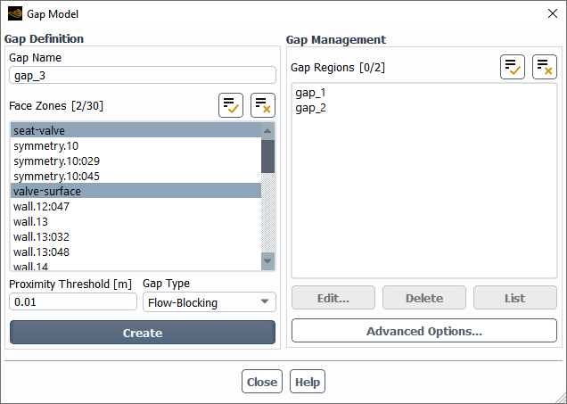
Create one or more gap regions using the input controls in the Gap Definition group box. For each one:

Provide a Gap Name. The name cannot consist solely of numbers.
Select two or more face zones (of type wall or symmetry) that could come in close proximity to each other from the Face Zones list; note that a given face zone may be used in multiple gap regions, but two or more face zones used in one gap region may not all be used in one other gap region. It is recommended that you use the minimum number of face zones as possible per gap region, as additional unnecessary face zones will adversely affect the calculation speed.
Specify a Proximity Threshold, that is, the maximum distance between the face zones when flow blockage / deceleration occurs.

Select one of the following from the Gap Type drop-down list:

Flow-Blocking
This type completely blocks the flow in the gap region, as a numerical zero-mass-flux boundary condition is applied at the boundary faces of the marked region so that the marked cells no longer participate in the solution. This can be appropriate for a valve that completely closes. It is recommended that you use this for meshes that only move translationally. Meshes that undergo rotational motion (such as gears or pumps) may experience divergence; in such cases, it may be possible to proceed using a larger proximity threshold so that the region of cells marked for blockage is larger (and you thus avoid creating "islands" of unmarked cells surrounded by marked cells).

Flow-Modeling

This type decelerates the flow in the cells of the marked region by manipulating the viscosity or source terms. Since it allows some leakage (though this can be negligible, based on your setup), it can be more robust if appropriately set up. It is recommended for meshes that undergo rotational motion, such as gears or pumps.

If you plan on controlling the flow based on the viscosity (the default method), you should specify an appropriate Gap Reynolds Number in order to obtain the desired level of sealing. A lower Gap Reynolds Number results in better sealing. You can determine a suitable value through trial and error during the simulation, or estimate it using the expected properties in the gap region according to the following equation:

(6–4)

where
	= gap Reynolds number
	= averaged density
	= averaged velocity
	= proximity threshold
	= averaged laminar viscosity

Click Create.

After you have created gap regions, you can revise the setup using the input controls in the Gap Management group box.
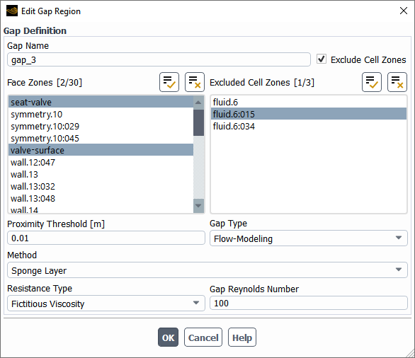
1. Revise a gap region by making a single selection from the Gap Regions list, clicking Edit..., and then completing the setup in the Edit Gap Region dialog box that opens.
  Figure 6.78: The Edit Gap Region Dialog Box
  
  In addition to the input controls you used when initially creating the gap region, the following settings can be defined:
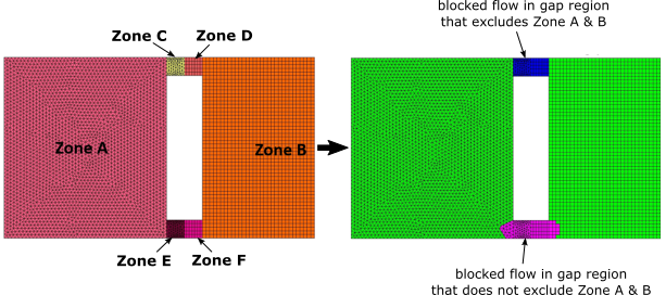
  - You can enable the Exclude Cell Zones option and then make selections from the Excluded Cell Zones list, in order to specify that cells in particular cell zones are not marked for flow blockage / deceleration as part of the gap region. In this way you can have greater control over the shape of the gap region, as shown in the figure that follows.
    Figure 6.79: Controlling Gap Shape by Excluding Zones
    
    Note: The Exclude Cell Zones option is automatically disabled for simulations that use overset meshes, as this combination is not supported.
  - If you selected Flow-Modeling for the Gap Type, you can select a Method:
    Sponge Layer
    This specifies that the viscosity inside the gap regions is scaled based on the specified Gap Reynolds Number. As the viscosity increases, the velocity in the gap region decreases. As part of this method, you can specify the Resistance Type, which affects the nature of the viscosity scaling: by default, the Fictitious Viscosity approach is used, as it is more robust and has less impact on thermal simulations. It scales the laminar viscosity inside the gap region during discretization of the viscous forces for the momentum equation; thus, its impact is explicitly seen in the velocity and pressure computation, and it has an implicit effect on the other solution fields through the changes in the velocity and pressure field. You can instead select the Real Viscosity approach, which changes the actual laminar viscosity inside the gap region based on your specified Gap Reynolds Number; therefore, the effect of modeling will be seen not only in flow equation but also in other equations. The flow inside the gap region modeled by this approach is indeed using a modified viscosity value over the course of the entire simulation.
    User-Defined Source
    This allows you to use a user-defined function (UDF) to specify the source terms for the momentum and energy equations in the gap region using the DEFINE_GAP_MODEL_SOURCE macro (for details, see DEFINE_GAP_MODEL_SOURCE in the Fluent Customization Manual). After you have compiled the UDF, you must then select it in the Gap Source Terms field. Note that interpreted UDFs are not supported.
2. To delete gap regions, select one or more in the Gap Regions list and click the Delete button.
3. To print a list in the console of the properties of gap regions, select one or more in the Gap Regions list and click the List button. Note that the number of cells marked for blockage / deceleration will not be updated until after you have generated data by initializing or calculating.
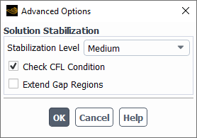
4. A gap region can introduce large gradients in the flow in the vicinity of the gap region boundary. You have the option of applying solution stabilization to improve the stability of the simulation by clicking the Advanced Options... button and selecting a Stabilization Level in the dialog box that opens. For each level, the solver adjusts the numerical settings, discretization schemes, under-relaxations, AMG settings, and so on, and controls the flow behavior in the vicinity of the gap regions; note that these changes are applied globally to all gap regions, and a level other than None will override the local stabilization applied by default to flow-modeling regions that use the Sponge Layer method. You should use the lowest level as possible, as the cost of computation increases with higher levels. Information about any changes made as part of this stabilization is printed in the console when you click OK.
  Figure 6.80: The Advanced Options Dialog Box
  
  You can enable the Check CFL Condition option if you want Fluent to determine a desirable acoustic Courant (CFL) number based on your selected Stabilization Level, and then provide a warning message in the console if this CFL number would require you to specify a smaller time step for the calculation in order to improve the solver stability.
  You can also enable the Extend Gap Regions if the shape of the marked cells is negatively affecting solution stability or convergence behavior. The gap regions will then be enlarged during marking by including additional cells in the vicinity of the gap interfaces.
When all of the gap regions are properly defined, click the OK button to close the Gap Model dialog box.

When you have a Flow-Modeling type gap region that uses the Sponge Layer method, by default a local stabilization is enabled to mitigate bad convergence behavior (though it can be disabled for individual gap regions using the define/gap-model/edit text command, or overridden generally through stabilization level set in the Advanced Options dialog box). You have the ability to revise the settings for all of the gap regions that use this local stabilization through the following text command:
define → gap-model → advanced-options → sponge-layer
- You can set the viscosity variation factor, which determines how much the viscosity linearly varies within the gap region as you approach the center. The default value of 0 produces maximum variability, which is appropriate when the gap size is larger and/or the viscosity within the gap region is very high compared to the flow domain. You can enter values closer to 1 (so that the viscosity is more fixed / constant throughout) when the gap is smaller and/or the viscosity is lower. Minimizing the variability restricts the flow better, but can lead to solution instability.
- You can set minimum limit for the velocity in the sponge layers. Viscosity scaling is disabled if the average velocity inside the gap region is less than this minimum.
- You can set the maximum limit for the viscosity change ratio in the sponge layers. The local stabilization method measures the variation of maximum viscosity to minimum viscosity inside the gap region, and constrains this ratio to be bounded between 0 and the value you enter. This can help avoid numerical instability when the variation of the viscosity inside the gap region is quite substantial compared to the flow viscosity.
During the solution, information about the gap model is printed in the console. You can set the level of detail that is provided by using the following text command:
define → gap-model → advanced-options → verbosity
Though it is not typically necessary, you can enable the following text command to make additional expert-level text commands available.
define → gap-model → advanced-options → expert?
The expert-level text commands include the following:
define/gap-model/advanced-options/enhanced-data-interpolation?
This can enable the use of enhanced data interpolation for updating information in gap regions. It may produce more accurate results, but with a higher computational cost.
define/gap-model/advanced-options/fill-data-in-gap-regions?
This can enable the interpolation of solution data throughout the gap regions.
define/gap-model/advanced-options/precise-gap-marking?
This can enable the use of a more accurate search algorithm for marking cells in gap regions. Note that it can be costly, particularly for 3D cases or those with a large number of cells inside the gap regions.
define/gap-model/advanced-options/reduce-gap-regions?
This can enable a more restrictive algorithm for marking cells in gap regions.
define/gap-model/advanced-options/render-flow-modeling-gaps?
This can disable the rendering of the solution in the cells of flow-modeling gap regions during postprocessing.
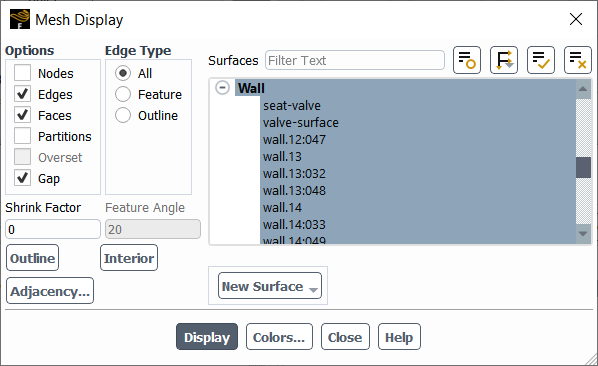
You can use the Mesh Display dialog box to view the mesh. By default, the complete mesh is displayed. If you enable the Gap option, only the cells in which flow is allowed are displayed (that is, those that are not marked for blockage in the gap region).
Domain → Mesh → Display
Figure 6.81: The Mesh Display Dialog Box for a Gap Model Simulation

Note: When displaying contours of postprocessing quantities, cells marked for blockage in a gap region are not shown (except for the Gap ID or Gap Type field variables), regardless of whether or not the Gap option is enabled in the Mesh Display dialog box.
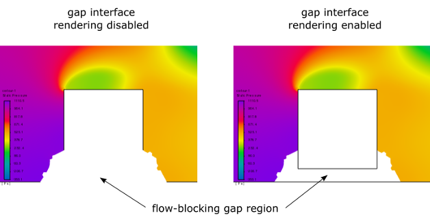
When displaying the mesh with contours, you can use the following text command to allow the rendering of the mesh surfaces inside the gap regions. Note that the solution is still not rendered inside the flow-blocking gap regions.
define → gap-model → advanced-options → render-gap-interface?
Figure 6.82: Contours and Mesh with a Flow-Blocking Gap
When postprocessing a gap model simulation, note that the Node Values option is not supported. The following field variables are available (under the Cell Info... category), and may visualize the gap regions:
- Gap ID
  This is the gap region ID, as identified using the List button in the Gap Model Dialog Box. All cells that are not marked for a gap region have a value of 0.
- Gap Type
  This is the type of gap region. Cells that are marked as part of a flow-blocking gap region have a value of 1, cells that are marked as part of a flow-modeling gap region have a value of 2, and cells that are not marked for a gap region have a value of 0.
- Flow-Blocking Gap Interface
  This identifies the interfaces of flow-blocking gap regions. All cells that have at least one face that applies the zero-mass-flux boundary for a gap region have a value of 1, whereas all other cells have a value of 0.

Note:

For steady-state simulations, if you have initialized the solution and then revise a gap region definition or delete a gap region such that there is a change in the cells that are marked for blockage / deceleration, then you must initialize again before proceeding.
It is recommended that you do not have two or more gap regions overlap (that is, mark the same cells), especially if they are not of the same Gap Type. If you enable the verbosity text command (define/gap-model/advanced-options/verbosity 1), you will receive a warning message in the console when gaps overlap. For flow-blocking gaps, you can replace the multiple overlapping gap regions with a single gap region that includes all of the related face zones and has a proximity threshold that is suitable for all.