


This section describes how to use sliding meshes, including restrictions and constraints, problem setup, solution strategies, and postprocessing.
Before beginning the problem setup in Ansys Fluent, be sure that the mesh you have created meets the following requirements:
The mesh must have a different cell zone for each portion of the domain that is sliding at a different speed.
The mesh interface must be situated such that there is no motion normal to it.
The mesh interface can be any shape (including a non-planar surface, in 3D), provided that the two interface boundaries are based on the same geometry. If there are sharp features in the mesh (for example, 90-degree angles), it is especially important that both sides of the interface closely follow that feature.
If you create a single mesh with multiple cell zones, you must be sure that each cell zone has a distinct face zone on the sliding boundary. The face zones for two adjacent cell zones will have the same position and shape, but one will correspond to one cell zone and one to the other. (Note that it is also possible to create a separate mesh file for each of the cell zones, and then merge them as described in Reading Multiple Mesh/Case/Data Files.)
If you are modeling a rotor/stator geometry using periodicity, the periodic angle of the mesh around the rotor blade(s) must be the same as that of the mesh around the stationary vane(s).
All periodic zones must be correctly oriented (either rotational or translational) before you create the mesh interface.
Note the following limitations if you want to use the periodic repeats option as part of the mesh interface:
The periodic repeats option is not supported if the interface zone is adjacent to a solid zone.
The edges of the second interface zone must be offset from the corresponding edges of the first interface zone by a uniform amount (either a uniform translational displacement or a uniform rotation angle).
Some portion of the two interface zones must overlap (that is, be spatially coincident).
The non-overlapping portions of the interface zones must have identical shape and dimensions at all times during the mesh motion.
One pair of conformal periodic zones must be adjacent to each of the interface zones. For example, when you calculate just one channel and blade of a fan, turbine, and so on, you must have conformal periodics on either side of the interface threads. This will not work with non-conformal periodics.
Note that for 3D cases, you cannot have more than one pair of conformal periodic zones adjacent to each of the interface zones.
You must not have a single sliding mesh interface where part of the interface is made up of a coupled two-sided wall, while another part is not coupled (that is, the normal interface treatment). In such cases, you must break the interface up into two interfaces: one that is a coupled interface, and the other that is a standard fluid-fluid interface. See Using a Non-Conformal Mesh in Ansys Fluent for information about creating coupled interfaces.
When using the sliding mesh technique, mass fluxes are interpolated from the sliding interface faces to the sliding boundary faces, which can affect the local mass balance at the sliding boundary. This can result in pressure field oscillations at the sliding boundary. These oscillations may be reduced by ensuring the surface mesh node distributions are similar on either side of the sliding boundaries. You can use the matching option (Matching Option), where applicable, to reduce solution oscillations at the sliding boundaries.
When using a sliding mesh to simulate flow through narrow gaps that open or close over time (such as in a valve or a rotary pump), you can use the gap model to block or decelerate the flow when the gaps are closed (as described in Controlling Flow in Narrow Gaps for Valves and Pumps).
For details about these restrictions and general information about how the sliding mesh model works in Ansys Fluent, see The Sliding Mesh Technique.
The steps for setting up a sliding mesh problem are listed below. (Note that this procedure includes only those steps necessary for the sliding mesh model itself; you must set up other models, boundary conditions, and so on, as usual.)
Enable the appropriate option for modeling transient flow. (See Performing Time-Dependent Calculations for details about the transient modeling capabilities in Ansys Fluent.)
 Setup
→ General
Setup
→ General Analysis
Type → Transient
Analysis
Type → Transient
Set the cell zone conditions for the sliding motion:
Setup →  Cell Zone
Conditions
Cell Zone
Conditions
In the Fluid Dialog Box or Solid Dialog Box of each moving fluid or solid zone, enable the Mesh Motion option and set the translational and/or rotational velocity under the Mesh Motion tab.
Important: Note that simultaneous translation and rotation can be modeled only if the rotation axis and the translation direction are the same (that is, the origin is fixed).
Note that the speed can be specified as a constant value or a transient profile. The transient profile may be in a file format, as described in Transient Cell Zone and Boundary Conditions, or a UDF macro, described in
DEFINE_TRANSIENT_PROFILEin the Fluent Customization Manual. Specifying the individual velocities as either a profile or a UDF allows you to specify a single component of the sliding motion individually. However, you can also specify the sliding motion using a user-defined function. This may prove to be quite convenient if you are modeling a more complicated motion, where the hooking of many different user-defined functions or profiles can be cumbersome.Note: If you decide to hook a UDF, then you will no longer have access to the rotation axis origin and direction, or the velocities.
Set the boundary conditions for the sliding motion:
Setup → Boundary
Conditions
Change the zone Type of the interface zones of adjacent cell zones to interface in the Boundary Conditions Task Page.
By default, the velocity of a wall is set to zero relative to the motion of the adjacent mesh. For walls bounding a moving mesh this results in a “no-slip” condition in the reference frame of the mesh. Therefore, you need not modify the wall velocity boundary conditions unless the wall is stationary in the absolute frame, and therefore moving in the relative frame. See Velocity Conditions for Moving Walls for details about wall motion.
See Cell Zone and Boundary Conditions for details about inputting cell zone and boundary conditions.
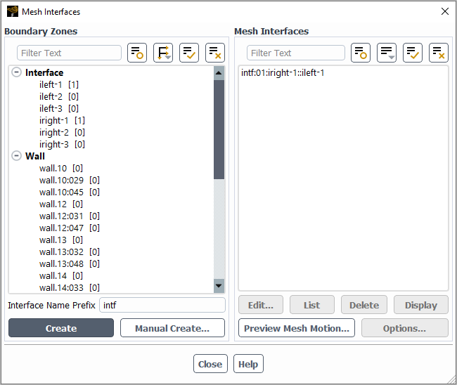
Define the mesh interfaces using the Mesh Interfaces Dialog Box (Figure 13.10: The Mesh Interfaces Dialog Box).
Setup → Mesh Interfaces
New...
To learn how to use the Mesh Interfaces dialog box, see Using a Non-Conformal Mesh in Ansys Fluent. Note that the Interface Options that are relevant for sliding meshes are Periodic Repeats, Coupled Wall, and Matching (for more information on these options, see Non-Conformal Mesh Calculations).
Preview the mesh motion using the Zone Motion dialog box, which can be opened from the Run Calculation task page.
Solution → Run Calculation
Preview Mesh Motion...
For details about using the Zone Motion dialog box, see Previewing the Dynamic Mesh.
(optional) After you have initialized or run the calculation, you can use the Moving Mesh Courant Number field variable (in the Velocity... category) to guide your solution. This field variable is a non-dimensional value that indicates the number of cells that might be swept in a single time step due to a mesh motion.
Important: When you have completed the problem setup, you should save an initial case file so that you can easily return to the original mesh position (that is, the positions before any sliding occurs). The mesh position is stored in the case file, so case files that you save at different times during the transient calculation will contain meshes at different positions.
Important: If you want to go from an MRF model setup to a sliding mesh setup, use the following text command:
mesh → modify-zones →
mrf-to-sliding-mesh
To successfully switch from an MRF to a sliding mesh, you must provide the ID of the fluid zone. Ansys Fluent identifies all the interior boundary zones of this fluid zone, as well as any adjacent fluid zones. Ansys Fluent changes these interior boundary zones into coupled walls, and then decouples these walls and changes them to interface zones. Ansys Fluent then changes the cell zone condition of the fluid zone to Moving Mesh in the Fluid Dialog Box. You do not need to do this if you have already created a mesh interface. The sliding mesh solution tends to be more robust than the MRF solution.
Note that all of the interfaces between the cells zones must be interior boundaries. This means that this text command cannot be used for a thermal simulation with solid zones adjacent to the MRF zone (for example, an MRF zone in contact with a solid volute).
You will begin the sliding mesh calculation by initializing the solution (as described in Initializing the Entire Flow Field Using Standard Initialization) and then specifying the time step size and number of time steps in the Run Calculation Task Page, as for any other transient calculation. (See Performing Time-Dependent Calculations for details about time-dependent solutions.) Note that the time step size in the initial case file is saved without clicking . Ansys Fluent will iterate on the current time step solution until satisfactory residual reduction is achieved, or the maximum number of iterations per time step is reached. When it advances to the next time step, the cell and wall zones will automatically be moved according to the specified translational or rotational velocities (as discussed in the previous section). The new interface-zone intersections will be computed automatically, and resultant interior/periodic/external boundary zones will be updated.
Note that you can run the MRF case using mesh interfaces with an appreciable loss of accuracy, doing so makes it easier to later on convert to a sliding mesh.
Note: The sliding mesh can be initialized with an MRF solution (rather using Standard or Hybrid initializations).
It is recommended that you preview the sliding mesh motion (as described in Previewing the Dynamic Mesh) before beginning your calculation. This can catch problems with the motion specification(s) before you begin the CFD calculation. Remember to save the case and initial data files before doing a mesh preview since the mesh position is altered once you do the preview. You can reread the initial condition case/data files to get back to the original mesh position.
Ansys Fluent’s automatic saving of case and data files (see Automatic Saving of Case and Data Files) can be used with the sliding mesh model. This provides a convenient way for you to save results at successive time steps for later postprocessing.
Important: You must save a case file each time you save a data file because the mesh position is stored in the case file. Since the mesh position changes with each time step, reading data for a given time step will require the case file at that time step so that the mesh will be in the proper position. You should also save your initial case file so that you can easily return to the mesh’s original position to restart the solution if desired.
For some problems (for example, rotor-stator interactions),
you may be interested in a time-periodic solution. That is, the startup
transient behavior may not be of interest to you. Once this startup
phase has passed, the flow will start to exhibit time-periodic behavior.
If  is the period of unsteadiness, then for some flow
property
is the period of unsteadiness, then for some flow
property  at a given point in the flow field:
 | (13–1) |
For rotating problems, the period (in seconds) can be calculated
by dividing the sector angle of the domain (in radians) by the rotor
speed (in radians/sec):  . For 2D rotor-stator problems,
  , where
  is the pitch and
  is the blade speed. The number of time steps in
a period can be determined by dividing the time period by the time
step size. When the solution field does not change from one period
to the next (for example, if the change is less than 5%), a time-periodic
solution has been reached.
is the blade speed. The number of time steps in
a period can be determined by dividing the time period by the time
step size. When the solution field does not change from one period
to the next (for example, if the change is less than 5%), a time-periodic
solution has been reached.
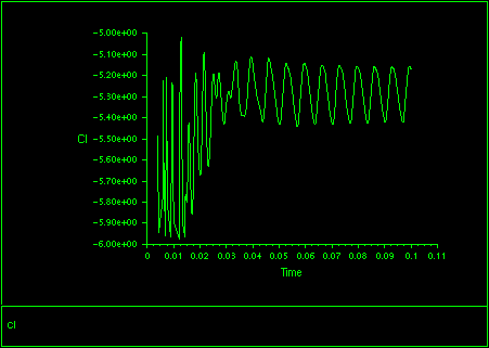
To determine how the solution changes from one period to the next, you must compare the solution at some point in the flow field over two periods. For example, if the time period is 10 seconds, you can compare the solution at a given point after 22 seconds with the solution after 32 seconds to see if a time-periodic solution has been reached. If not, you can continue the calculation for another period and compare the solutions after 32 and 42 seconds, and so on until you see little or no change from one period to the next. You can also track global quantities, such as lift and drag coefficients and mass flow, in the same manner. Figure 13.11: Lift Coefficient Plot for a Time-Periodic Solution shows a lift coefficient plot for a time-periodic solution.
The final time-periodic solution is independent of the size of the time steps taken during the initial stages of the solution procedure. You can therefore define a “large” time step size in the initial stages of the calculation, since you are not interested in a time-accurate solution for the startup phase of the flow. Starting out with a large time step size will allow the solution to become time-periodic more quickly. As the solution becomes time-periodic, however, you should reduce size of the time steps in order to achieve a time-accurate result.
Important: If you are solving with second-order time accuracy, the temporal accuracy of the solution will be affected if you change the time step size during the calculation. You may start out with a larger time step size, but you should not change the time step size by more than 20% during the solution process. You should not change the time step size at all during the last several periods to ensure that the solution has approached a time-periodic state.
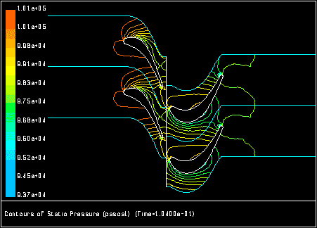
Postprocessing for sliding mesh problems is the same as for other transient problems. You will read in the case and data file for the time of interest and display and report results as usual. For spatially-periodic problems, you may want to use periodic repeats (set in the Views Dialog Box, as described in Controlling the Display State and Modifying the View) to display the geometry. Figure 13.12: Contours of Static Pressure for the Rotor-Stator Example shows the flow field for the rotor-stator example in Figure 13.4: Initial Position of the Meshes) at one instant in time, using 1 periodic repeat.
When displaying velocity vectors, note that absolute velocities (that is, velocities in the inertial, or laboratory, reference frame) are displayed by default. You may also choose to display relative velocities by selecting Relative Velocity in the Vectors of drop-down list in the Vectors Dialog Box. In this case, velocities relative to the translational/rotational velocity of the “reference zone” (specified in the Reference Values Task Page) will be displayed. (The velocity of the reference zone is the velocity defined in the Fluid Dialog Box for that zone.)
Note that you cannot create zone surfaces for the intersection
boundaries (that is, the interior/periodic/external zones created
from the intersection of the interface zones). You may instead create
zone surfaces for the interface zones. Data displayed on these surfaces
will be “one-sided”. That is, nodes on the interface
zones will “see” only the cells on one side of the mesh
interface, and slight discontinuities may appear when you plot contour
lines across the interface. Note also that, for non-planar interface
shapes in 3D, you may see small gaps in your plots of filled contours.
These discontinuities and gaps are only graphical in nature. The solution
does not have these discontinuities or gaps. To eliminate these discontinuities
for postprocessing purposes only, you can use the define/mesh-interfaces/enforce-continuity-after-bc? text command, which will ensure that continuity will take precedence
over the boundary condition.
You can also generate a plot of circumferential averages in Ansys Fluent. This allows you to find the average value of a quantity at several different radial or axial positions in your model. Ansys Fluent computes the average of the quantity over a specified circumferential area, and then plots the average against the radial or axial coordinate. For more information on generating XY plots of circumferential averages, see XY Plots of Circumferential Averages.
Sliding mesh results can be analyzed by employing the time averaging (or RMSE averaging) option (Data Sampling for Time Statistics) in the Run Calculation task page. This will compute time averages for velocity, pressure, temperature, and turbulence. You must plan ahead since you have to engage the time averaging after the solution has become time-periodic and run for at least one period of the oscillating flow field.