


The primary inputs that you must provide for the discrete phase calculations in Ansys Fluent are the initial conditions that define the starting positions, velocities, and other parameters for each particle stream and the physical effects acting on the particle streams, requiring additional particle properties. You will define the initial conditions for a particle/droplet stream by creating an “injection” and assigning properties to it.
The required initial conditions depend on the injection type, while the physical effects are selected by choosing an appropriate particle type. For some injection types you can provide a particle size distribution, like the Rosin-Rammler distribution, see Using the Rosin-Rammler Diameter Distribution Method.
The initial conditions provide the starting values for all of the dependent discrete phase variables that describe the instantaneous conditions of an individual particle, and include the following:
position (
 ,
,  ,
,  coordinates) of the particle
velocities (
 ,
,  ,
,  ) of the particle
Velocity magnitudes and spray cone angle can also be used (in 3D) to define the initial velocities (see Point Properties for Cone Injections). For moving reference frames, relative velocities should be specified.
diameter of the particle,

temperature of the particle,

mass flow rate of the particle stream that will follow the trajectory of the individual particle/droplet,
 (required
only for coupled calculations)
(required
only for coupled calculations)additional parameters if one of the atomizer models described in Atomizer Model Theory in the Theory Guide is used for the injection
Important: When an atomizer model is selected, you will not specify initial diameter, velocity, and position quantities for the particles due to the complexities of sheet and ligament breakup. Instead of initial conditions, the quantities you will specify for the atomizer models are global parameters.
These dependent variables (temperature, diameter, and so on) are updated according to the equations of motion (Particle Motion Theory in the Theory Guide) and according to the heat/mass transfer relations applied (Laws for Heat and Mass Exchange in the Theory Guide) as the particle/droplet moves along its trajectory. You can define any number of different sets of initial conditions for discrete phase particles/droplets provided that your computer has sufficient memory.
For the setup of transient particle cases, the point properties for mass flow and velocity can be specified using transient profiles (see Point Properties for Transient Injections).
For additional information, see the following sections:
- 24.3.1. Injection Types
- 24.3.2. Particle Types
- 24.3.3. Point Properties for Single Injections
- 24.3.4. Point Properties for Group Injections
- 24.3.5. Point Properties for Cone Injections
- 24.3.6. Point Properties for Surface Injections
- 24.3.7. Point Properties for Volume Injections
- 24.3.8. Point Properties for Plain-Orifice Atomizer Injections
- 24.3.9. Point Properties for Pressure-Swirl Atomizer Injections
- 24.3.10. Point Properties for Air-Blast/Air-Assist Atomizer Injections
- 24.3.11. Point Properties for Flat-Fan Atomizer Injections
- 24.3.12. Point Properties for Effervescent Atomizer Injections
- 24.3.13. Point Properties for File Injections
- 24.3.14. Point Properties for Condensate Injections
- 24.3.15. Using the Rosin-Rammler Diameter Distribution Method
- 24.3.16. Using the Tabulated (Discrete) Diameter Distribution
- 24.3.17. Creating and Modifying Injections
- 24.3.18. Defining Injection Properties
- 24.3.19. Specifying Injection-Specific Physical Models
- 24.3.20. Specifying Turbulent Dispersion of Particles
- 24.3.21. Custom Particle Laws
- 24.3.22. Defining Properties Common to More than One Injection
- 24.3.23. Point Properties for Transient Injections
Ansys Fluent provides the following types of injections:
single
group
cone (only for 3D cases)
surface
volume (only for non-DEM 3D cases with unsteady particle tracking)
plain-orifice atomizer
pressure-swirl atomizer
air-blast-atomizer
flat-fan-atomizer
effervescent-atomizer
file
condensate
For each non-atomizer injection type, you will specify each of the initial conditions listed in Setting Initial Conditions for the Discrete Phase, the type of particle that possesses these initial conditions, and any other relevant parameters for the particle type chosen.
When defining injection point properties for the following injection types:
single
group
all cone injections
all atomizer injections
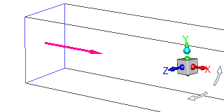
you can interactively preview the current injection position and orientation in the graphics window prior to saving the settings. When you click Update Injection Display in the Set Injection Properties dialog box or Set Multiple Injection Properties dialog box, Ansys Fluent will apply the current settings to the injection display. Once you click in the Set Injection Properties dialog box or in the Set Multiple Injection Properties dialog box, the injection properties will be saved, and the graphics window will be once more updated. When you open the Set Injection Properties dialog box for the existing injection, Ansys Fluent will also automatically display the injection in the graphics window.
The injection position and orientation will not be displayed if you use profiles to specify the injection position and direction. If you use the DEFINE_DPM_INJECTION_INIT user-defined function, the displayed injection position and orientation will reflect only the default point properties for the specific injection type.
Use the following guidelines for choosing the injection type:
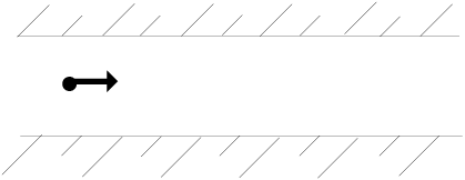
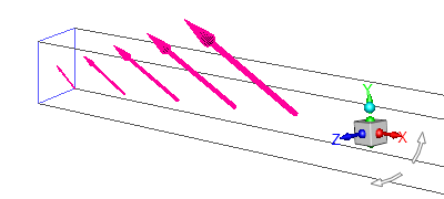
Create a single injection when you want to specify a single value for each of the initial conditions (Figure 24.13: Particle Injection Defining a Single Particle Stream).
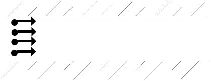
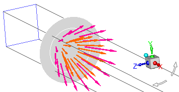
Create a group injection (Figure 24.14: Particle Injection Defining an Initial Spatial Distribution of the Particle Streams) when you want to define a range for one or more of the initial conditions (for example, a range of diameters or a range of initial positions).
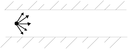
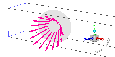
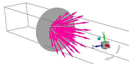
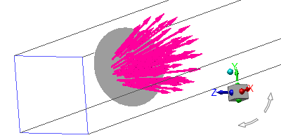
To define cone injections in 3D problems, create a cone injection and specify a particle release pattern (point, hollow, ring, or solid) (Figure 24.15: Particle Injection Defining an Initial Spray Distribution of the Particle Velocity).
Create a surface injection to release particles from a surface (either a zone surface or a surface you have defined using Create in the Domain ribbon tab (Surface group box)). A particle stream will be released from each facet of the surface. You can use the Bounded and Sample Points options in the Plane Surface dialog box to create injections from a rectangular mesh of particles in 3D (see Plane Surfaces for details).
If you want to create a spray atomizer, you can use one of the predefined atomizer injections (plain-orifice, pressure-swirl, air-blast, flat-fan, or effervescent).
Create a volume injection if you want to populate a volume zone or bounding geometry with particles. You can either choose one or several volume zones created when generating the mesh for your case or define a bounding geometry such as sphere, cylinder, cone, and hexahedron. See Defining Injection Properties for details.
Create a file injection to release particles with property settings stored in a file.
If you are modeling film condensation, create a condensate injection to define the vapor-liquid material pair and other modeling settings for the film condensation process.
Particle initial conditions (position, velocity, diameter, temperature, and mass flow rate) can also be read from an external file if none of the injection types listed above can be used to describe your injection distribution.
The inputs for setting injections are described in detail in Defining Injection Properties.
When you define a set of initial conditions (as described in Defining Injection Properties), you will need to specify the type of particle. The particle types available to you depend on the range of physical models that you have defined.
A massless particle is a discrete element that follows the flow and temperature of the continuous phase. As it has no mass, it has no associated physical properties, and no force is exerted on it. However, you can assign a User-Defined Law to be applied to the massless particle. The massless particle type is available with all Ansys Fluent models.
An inert particle is a discrete phase element (particle, droplet, or bubble) that obeys the force balance (Equation 12–1 in the Theory Guide) and is subject to heating or cooling via Law 1 (Inert Heating or Cooling (Law 1/Law 6) in the Theory Guide). The inert type is available for all Ansys Fluent models.
A droplet particle is a liquid droplet in a continuous-phase gas flow that obeys the force balance (Equation 12–1 in the Theory Guide) and that experiences heating/cooling via Law 1 followed by vaporization and boiling via Laws 2 and 3 (Droplet Vaporization (Law 2) and Droplet Boiling (Law 3) in the Theory Guide). The droplet type is available when heat transfer is being modeled and at least two chemical species are active or the non-premixed or partially premixed combustion model is active. You should use the ideal gas law to define the gas-phase density (in the Create/Edit Materials dialog box, as discussed in Density Inputs for the Incompressible Ideal Gas Law) when you select the droplet type.
A combusting particle is a solid particle that obeys the force balance (Equation 12–1), and, after an initial phase of inert heating (Law 1), undergoes devolatization (Devolatilization (Law 4)) and then a heterogeneous surface reaction via Law 5 (Surface Combustion (Law 5) in the Theory Guide). Finally, the nonvolatile portion of a combusting particle is subject to inert heating via Law 6. You can also include an evaporating material with the combusting particle by selecting the Wet Combustion option in the Set Injection Properties Dialog Box. This allows you to include a material that evaporates and boils via Laws 2 and 3 (Droplet Vaporization (Law 2) and Droplet Boiling (Law 3) in the Theory Guide) before devolatilization of the particle material begins. The combusting type is available when heat transfer is being modeled and at least two chemical species are active or the non-premixed combustion model is active. You should use the ideal gas law to define the gas-phase density (in the Create/Edit Materials Dialog Box) when you select the combusting particle type.
A multicomponent particle is, as the name implies, a particle containing a mixture of several components or species. The conservation equations of all components, the energy equation, and vapor-liquid-equilibrium at the multicomponent particle surface form a coupled system of differential equations. You should use the volume weighted mixing law to define the particle mixture density (in the Create/Edit Materials Dialog Box) when you select the particle-mixture material type. Law 7, the multicomponent law (Multicomponent Particle Definition (Law 7) in the Theory Guide) is used for the evaporating and boiling components of the particle.
When all volatile components are evaporated via Law 7, multicomponent particles can participate in chemical reactions as described in Multicomponent Particles with Chemical Reactions (Law 8). See Multicomponent Particles with Chemical Reactions in the Fluent Theory Guide for reaction types that multicomponent particles can undergo and reaction models that are available in Ansys Fluent.
The types of particles and the laws they are subjected to are summarized in the table below.
| Particle Type | Description | Laws Activated |
|---|---|---|
| Massless | – | – |
| Inert | inert/heating or cooling | 1, 6 |
| Droplet | heating/evaporation/boiling | 1, 2, 3, 6 |
| Combusting | heating; evolution of volatiles/swelling; heterogeneous surface reaction | 1, 4, 5, 6 |
| Multicomponent | multicomponent droplets/particles | 7, 8 |
For a single injection, you will define the following initial conditions for the particle stream under the Point Properties heading (in the Set Injection Properties Dialog Box):
position
Set the
 ,
,  , and
, and  positions of the injected stream
along the Cartesian axes of the problem geometry in the X-, Y-, and Z-Position fields. (Z-Position will appear only for 3D
problems.)
positions of the injected stream
along the Cartesian axes of the problem geometry in the X-, Y-, and Z-Position fields. (Z-Position will appear only for 3D
problems.)velocity
Set the
 ,
,  , and
, and  components of the stream’s
initial velocity in the X-, Y-, and Z-Velocity fields. (Z-Velocity will appear only for 3D problems.)
components of the stream’s
initial velocity in the X-, Y-, and Z-Velocity fields. (Z-Velocity will appear only for 3D problems.)angular velocity (available when particle rotation is enabled (see Particle Rotation))
Set the
 ,
,  , and
, and  components of the stream’s initial velocity
in the X-, Y-, and Z-Angular-Velocity fields. (Only Z-Angular-Velocity will appear for 2D problems, because rotation in 2D occurs in the
plane, that is, the rotation vector is normal to the plane.)
components of the stream’s initial velocity
in the X-, Y-, and Z-Angular-Velocity fields. (Only Z-Angular-Velocity will appear for 2D problems, because rotation in 2D occurs in the
plane, that is, the rotation vector is normal to the plane.)diameter
Set the initial diameter of the injected particle stream in the Diameter field.
temperature
Set the initial (absolute) temperature of the injected particle stream in the Temperature field.
mass flow rate
For coupled phase calculations (see Solution Strategies for the Discrete Phase), set the mass of particles per unit time that follows the trajectory defined by the injection in the Flow Rate field. Note that in axisymmetric problems the mass flow rate is defined per
 radians
and in 2D problems per unit meter depth (regardless of the reference
value for length).
radians
and in 2D problems per unit meter depth (regardless of the reference
value for length).duration of injection
For unsteady particle tracking (see Steady/Transient Treatment of Particles), set the starting and ending time for the injection in the Start Time and Stop Time fields. When In-Cylinder mesh motion is enabled, set the starting and ending crank angles for the injection in the Start Crank Angle and Stop Crank Angle fields. The values you enter are for one complete engine cycle. In subsequent cycles, the injection will be started and stopped according to Equation 13–30, where
 corresponds
to the injection start or end crank angle.
corresponds
to the injection start or end crank angle.time delay for reinjecting particles
If the injection is used only for reinjecting particles (Reinjection Only is enabled), you can specify Reinjection Time Delay. See The reinject Boundary Condition for details.
For the massless particle type, you will only need to define the position of the injection. The particle injection velocity is set by the solver equal to the velocity of the continuous phase at the injection point.
If you want to randomly distribute the initial placement of the particles, you can enable Stagger Positions and specify Stagger Radius to define the particle release region. For more information on spatial staggering, see Staggering of Particles in Space and Time. This option is disabled by default.
For group injections, you will define the properties position, velocity, angular velocity (available when particle rotation is enabled (see Particle Rotation)), diameter, temperature, and flow rate for the First Point and Last Point in the group. That is, you will define a range of values,  through
  , for each initial condition
  by setting values for
  and
and  . Ansys Fluent assigns a value of
  to the
  th injection in the group using a linear variation between the first and last values for
  :
:
 | (24–7) |
Thus, for example, if your group consists of 5 particle streams
and you define a range for the initial  location from 0.2 to 0.6 meters,
the initial
location from 0.2 to 0.6 meters,
the initial  location of each stream is as follows:
Stream 1:
 = 0.2 meters
Stream 2:
 = 0.3 meters
Stream 3:
 = 0.4 meters
Stream 4:
 = 0.5 meters
Stream 5:
 = 0.6 meters
Important: In general, you should supply a range for only one of the initial conditions in a given group—leaving all other conditions fixed while a single condition varies among the stream numbers of the group. Otherwise you may find, for example, that your simultaneous inputs of a spatial distribution and a size distribution have placed the small droplets at the beginning of the spatial range and the large droplets at the end of the spatial range.
The specified flow rate is defined per particle stream and can also be interpolated using Equation 24–7. When a Rosin-Rammler sized distribution is specified the total flow rate will be specified.
For the massless particle type, you will only need to define the first and last point of the injection group position. The particle velocities are set by the solver equal to the velocity of the continuous phase at the injection points.
If the injections are used only for reinjecting particles (Reinjection Only is enabled), you can specify Reinjection Time Delay. See The reinject Boundary Condition for details.
Note that you can use a different method for defining the size distribution of the particles, as discussed below.
To randomly distribute the initial placement of the particles, enable Stagger Positions and specify Stagger Radius to define the particle release region. For more information on spatial staggering, see Staggering of Particles in Space and Time. This option is disabled by default.
In 3D problems, you can define the following types of particle stream cones:
point-cone
hollow-cone
ring-cone
solid-cone
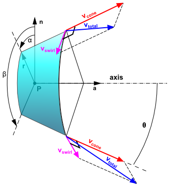
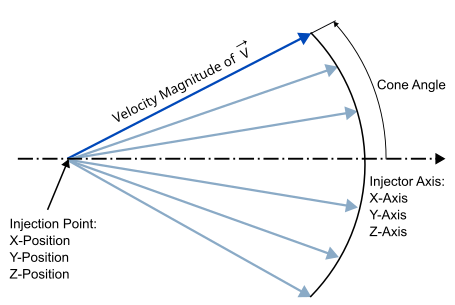
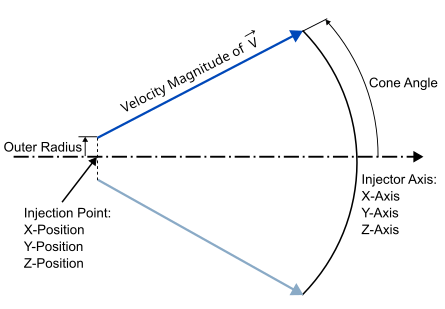
The particles are released from a 2D region that may be a point, a circle, or an annulus. Its geometry, location, and orientation as well as the shape of the spray cone are defined by the injection parameters. Once you select a cone injection type from the Cone Type drop-down list, (the Cone Injector Parameters group box in the Point Properties tab of the Set Injection Properties dialog box), the parameters specific to the selected injection type will be displayed. These inputs are summarized below. Refer to Figure 24.16: Cone Injector Geometry for an illustration of the geometry.
position
Set the coordinates of the origin of the spray cone in the X-, Y-, and Z-Position fields (
 in Figure 24.16: Cone Injector Geometry)
diameter
Set the diameter of the particles in the stream in the Diameter field.
temperature
Set the temperature of the streams in the Temperature field.
duration of injection
For unsteady particle tracking (see Steady/Transient Treatment of Particles), set the starting and ending time for the injection in the Start Time and Stop Time fields. When In-Cylinder mesh motion is enabled, set the starting and ending crank angles for the injection in the Start Crank Angle and Stop Crank Angle fields.
axis
Set the
 ,
,  , and
, and  components of the vector defining
the cone’s axis in the X-Axis, Y-Axis, and Z-Axis fields. (
components of the vector defining
the cone’s axis in the X-Axis, Y-Axis, and Z-Axis fields. ( in Figure 24.16: Cone Injector Geometry)
velocity
Set the velocity magnitude of the particle streams that will be oriented along the specified spray cone in the Velocity Magnitude field. (
 in Figure 24.16: Cone Injector Geometry)
angular velocity
Set the angular velocity magnitude of the particle streams that will be oriented along the specified spray cone in the Angular Velocity Magnitude field.
cone angle
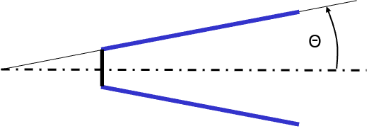
Set the included half-angle of the spray cone in the Cone Angle field. (
 in Figure 24.16: Cone Injector Geometry)
dispersion angle
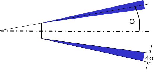
For hollow-cone, you can optionally specify Dispersion Angle (default: 0). A non-zero value of the dispersion angle results in a distribution of the spray angle, that is, spray clustered about the mean cone angle using a Gaussian distribution with 0 mean and +/- 2 standard deviation (
 in Figure 24.18: Hollow Cone With Specified Cone Angle And Dispersion Angle).
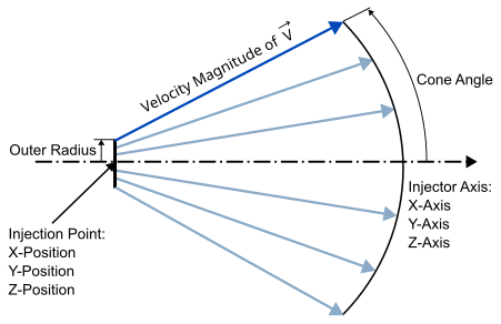
 radii
For hollow-cone, ring-cone, and solid-cone injections, specify the Outer Radius.
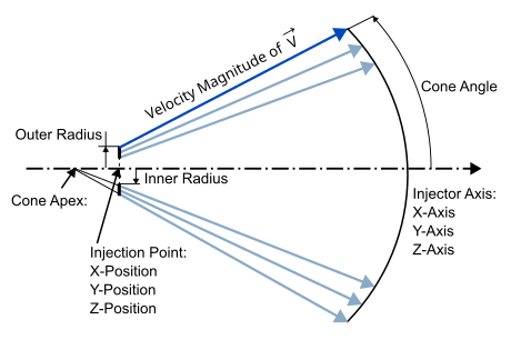
For ring-cone injections, specify a nonzero Inner Radius to model injectors that do not emanate from a single point. The particles will be distributed about the axis with the specified radius. (
 in Figure 24.16: Cone Injector Geometry)
swirl fraction (hollow cone only)
Set the swirl fraction, which determines the relative magnitude of the swirl velocity, in the Swirl Fraction field.
The direction of the swirl component is defined using the right-hand rule about the cone axis (a negative value for the swirl fraction can be used to reverse the swirl direction).
mass flow rate
For coupled calculations, set the total mass flow rate for the streams in the spray cone in the Total Flow Rate field. Note that for a 3D sector, the flow rate must be appropriate for the sector defined by the Azimuthal Start Angle and Azimuthal Stop Angle.
azimuthal angles
For 3D sectors, set the Azimuthal Start Angle and Azimuthal Stop Angle to define the sector. (
 and
and  , respectively, in Figure 24.16: Cone Injector Geometry).
The Azimuthal Start Angle and Azimuthal Stop Angle are specified with respect to a reference vector,
 , that is orthogonal to both the cone axis
and the global X axis. The reference vector,
, that is orthogonal to both the cone axis
and the global X axis. The reference vector,  , can be determined as the cross product of the cone
axis and the global X axis.
, can be determined as the cross product of the cone
axis and the global X axis.where
 is a unit vector along the global X axis. In the
case that the cone axis is along the X axis, then
is a unit vector along the global X axis. In the
case that the cone axis is along the X axis, then  is along the Y axis.
time delay for reinjecting particles
If the injection is used only for reinjecting particles (Reinjection Only is enabled), you can specify Reinjection Time Delay. See The reinject Boundary Condition for details.


In addition to the above parameters, you can select the following options:
Uniform Massflow Distribution (solid-cone or ring-cone): Specifies a uniform spatial distribution of mass over the cross-section of a cone. This is especially important when the mesh cell size is smaller than the particle diameter or another characteristic size. This option is enabled by default.
Stagger Positions: Specifies a random spatial distribution of particle streams.
For hollow-cone injections, you must also specify Stagger Radius to define the region over which particle release points are staggered in space. You can also enable the Stagger in Injection Plane Only option to restrict the spatial staggering of the initial particle positions to purely the radial direction of the spray. The spatial staggering clusters the initial particle positions about the outer radius of the hollow cone using a Gaussian distribution with 0 mean and +/- 2 standard deviation.
For more information on spatial staggering, see Staggering of Particles in Space and Time. This option is disabled by default.
The distribution of the velocity directions in the particle streams for the point-cone, ring-cone, and solid-cone injections is random. Furthermore, duplicating this injection may not necessarily result in the same distribution, at the same location.
Important: For transient calculations, the spatial distribution of streams at the initial injection location is recalculated at each time step. Sampling different possible trajectories allows a more accurate representation of a point, ring, or solid cone using fewer computational parcels. For steady-state calculations, the trajectories are initialized one time and kept the same for subsequent DPM iterations. The trajectories are recalculated when a change in the Injections dialog box occurs or when a case and data file are saved. If the residuals and solution change when a small change is made to the injection or when a case and data file are saved, it may mean that there are not enough trajectories being used to represent the point, ring, or solid cone with sufficient accuracy.
Note that you may want to define multiple spray cones emanating from the same initial location in order to specify a known size distribution of the spray or to include a known range of cone angles.
For the massless particle type, you will only need to define position, axis, cone angle, azimuthal angles, and radius. The particle velocities are set by the solver equal to the velocity of the continuous phase at the injection points.
Some additional details about injection point properties and other inputs for different cone injection types are provided below.
Point injections
Number of Streams parcels will be injected from the injection point.
The envelope of the particle trajectories forms a cone with a total opening angle of 2*Cone Angle.
Solid injections
Number of Streams parcels will be injected from the injection plane.
Parcels start from any radial distance within the injection plane (
 ).
). The envelope of the particle trajectories forms a cone with a total opening angle of 2*Cone Angle.
Ring injections
Number of Streams parcels will be injected from the injection plane.
Parcels start from any radial distance within the injection plane (
 ).
). The inner envelope of the particle trajectories results from the position of the cone apex of the outer envelope (which is computed by the solver from the injection point properties) and the inner radius of the injection plane.
Hollow injections
Number of Streams parcels will be injected from the plane circumference.
Parcels start from a fixed radial distance (
 ).
). The outer envelope of the particle trajectories form a cone with a total opening angle of 2*Cone Angle.
For surface injections, you will define all the properties described in Point Properties for Single Injections except for the initial position of the particle streams. The initial positions of the particles will be the location of the data points on the specified surface(s). Note that you will set the Total Flow Rate of all particles released from the surface (required for coupled calculations only). If you want, you can scale the individual mass flow rates of the particles by the ratio of the area of the face they are released from to the total area of the surface. To scale the mass flow rates, select the Scale Flow Rate By Face Area option under Point Properties. For the massless particle type, you will not need to enter any information to define a surface injection. The particle velocities are set by the solver equal to the velocities of the continuous phase at the injection points.
Note that many surfaces have nonuniform distributions of points. If you want to generate a uniform spatial distribution of particle streams released from a surface in 3D, you can create a bounded plane surface with a uniform distribution using the Plane Surface Dialog Box, as described in Plane Surfaces. In 2D, you can create a rake using the Line/Rake Surface Dialog Box, as described in Line and Rake Surfaces.
If you want to inject particles from positions distributed randomly over the selected boundary surfaces, enable Randomize Starting Points (Surface Options group box).
In addition to the option of scaling the flow rate by the face area, the normal direction of a face can be used for the injection direction. To use the face normal direction for the injection direction, select the Inject Using Face Normal Direction option under Point Properties (Figure 24.33: Setting Surface Injection Properties). Once this option is selected, you only need to specify the velocity magnitude of the injection, not the individual components of the velocity magnitude.
Important:
Only surface injections from boundary surfaces will be moved with the mesh when a sliding mesh, or a moving or deforming mesh is being used.
For simulations that involve dynamic meshes, sliding meshes, or automatic adaption, only zonal surfaces can be selected.
A nonuniform size distribution can be used for surface injections, as described below.
The Rosin-Rammler size distributions described in Using the Rosin-Rammler Diameter Distribution Method for group injections is also available for surface injections. If you select one of the Rosin-Rammler diameter distributions (rosin-rammler or rosin-rammler-logarithmic), you will need to specify the following parameters under Point Properties, in addition to the initial velocity, temperature, and total flow rate:
Min. Diameter
This is the smallest diameter to be considered in the size distribution.
Max. Diameter
This is the largest diameter to be considered in the size distribution.
Mean Diameter
This is the size parameter,
 , in the Rosin-Rammler equation (Equation 24–9).
Spread Parameter
This is the exponential parameter,
 , in Equation 24–9.
Number of Diameters
This is the number of diameters in each distribution (that is, the number of different diameters in the stream injected from each face of the surface).
Ansys Fluent will inject streams of particles from each face on the surface, with diameters defined by the Rosin-Rammler distribution function. The total number of injection streams tracked for the surface injection will be equal to the number of diameters in each distribution (Number of Diameters) multiplied by the number of faces on the surface.
For unsteady particle tracking, if you want to inject wall film particles from surfaces:
For a surface(s) from which wall film particles are released, specify the wall-film boundary condition in the DPM tab of the Wall dialog box. See Setting the Lagrangian Wall Film Model for details.
In the Set Injection Properties dialog box, make sure that surface is selected as Injection Type.
In the Point Properties tab, enable the Inject Wallfilm Particles (Wallfilm group box).
The Injection Surfaces multiple-selection list only displays the surfaces with the wall-film boundary condition.
In the Injection Surfaces multiple-selection list, select the surface(s) from which the wall-film particles will be released.
Specify other injection properties as appropriate for your case.
The X-, Y- or Z-Velocity will be projected in a directions parallel to each wall surface.
Note that the following options are not supported with the Inject Wallfilm Particles option:
Stagger Positions
Wall film particles must stay on the wall surface and are not allowed to hover above or below it.
Inject Using Face Normal Direction
The velocity of the wall-film particles should not be equal to the velocity of the particle release surface.
For volume injections, you will define all the properties described in Point Properties for Single Injections except for the initial positions of the particle streams. The initial positions of the particle parcels will be randomly chosen from points uniformly distributed in the volume zone or bounding geometry. See Defining Injection Properties for details.
By default, the Total Flow Rate of the parcel to be injected into the particle release region is to be specified. If you prefer to specify the Total Mass of the parcel instead, enable the Use Mass Instead of Flow Rate option. If you enable the Use Volume Fraction Instead of Flow Rate option and specify Volume Fraction (rather than Total Mass Rate or Total Mass) in the Set Injection Properties dialog box (Point Properties tab). During simulation, parcels are introduced into the specified zones or bounding shape until either the specified Volume Fraction or Injection Limit per Cell is reached.
For the massless particle type, no input is required from you to define a volume injection. The particle velocities are set by the solver equal to the velocities of the continuous phase at the injection points.
Important: If the injection Stop Time and Start Time are in different fluid flow time steps, then the particles will be injected at once in the Fluid Time Step that includes the middle of the injection time interval [Start Time, Stop Time].
For DDPM cases, the injection Start Time and Stop Time must be inside the same Fluid Flow Time Step; otherwise, no particles will be injected.
The Rosin-Rammler size distributions described in Using the Rosin-Rammler Diameter Distribution Method for group injections is also available for volume injections. When you select rosin-rammler or rosin-rammler-logarithmic as Diameter Distribution, you need to specify additional point properties parameters described in Using the Rosin-Rammler Diameter Distribution Method for Surface Injections.
Ansys Fluent will inject particle parcels uniformly randomly distributed in either a specified zone or bounding geometry with diameters defined by the Rosin-Rammler distribution function. The total number of injected particle parcels tracked for the volume injection will be equal to the Number of Diameters in each distribution multiplied by either the number-of-starting-points or the parcels-per-cell specified for the zone or number-of-starting-points specified for the bounding geometry.
For a plain-orifice atomizer injection, you will define the following initial conditions under Point Properties:
position
Set the
 ,
,  , and
, and  positions of the injected stream
along the Cartesian axes of the problem geometry in the X-Position, Y-Position, and Z-Position fields. (Z-Position will
appear only for 3D problems).
positions of the injected stream
along the Cartesian axes of the problem geometry in the X-Position, Y-Position, and Z-Position fields. (Z-Position will
appear only for 3D problems).axis (3D only)
Set the
 ,
,  , and
, and  components of the vector defining
the axis of the orifice in the X-Axis, Y-Axis, and Z-Axis fields.
components of the vector defining
the axis of the orifice in the X-Axis, Y-Axis, and Z-Axis fields.temperature
Set the temperature of the streams in the Temperature field.
mass flow rate
Set the total mass flow rate for the streams in the atomizer in the Flow Rate field. Note that in 3D sectors, the flow rate must be appropriate for the sector defined by the Azimuthal Start Angle and Azimuthal Stop Angle.
duration of injection
For unsteady particle tracking (see Steady/Transient Treatment of Particles), set the starting and ending time for the injection in the Start Time and Stop Time fields. When In-Cylinder mesh motion is enabled, set the starting and ending crank angles for the injection in the Start Crank Angle and Stop Crank Angle fields.
vapor pressure
Set the vapor pressure governing the flow through the internal orifice (
 in Table 12.7: List of Governing Parameters for Internal Nozzle Flow in the Theory Guide) in the Vapor Pressure field.
diameter
Set the diameter of the orifice in the Injector Inner Diameter field (
 in Table 12.7: List of Governing Parameters for Internal Nozzle Flow in the Theory Guide).
orifice length
Set the length of the orifice in the Orifice Length field (
 in Table 12.7: List of Governing Parameters for Internal Nozzle Flow in the Theory Guide).
radius of curvature
Set the radius of curvature of the inlet corner in the Corner Radius of Curvature field (
 in Table 12.7: List of Governing Parameters for Internal Nozzle Flow in the Theory Guide).
nozzle parameter
Set the constant for the spray angle correlation in the Constant A field (
 in Equation 12–369 in the Theory Guide).
azimuthal angles
For 3D sectors, set the Azimuthal Start Angle and Azimuthal Stop Angle.
time delay for reinjecting particles
If the injection is used only for reinjecting particles (Reinjection Only is enabled), you can specify Reinjection Time Delay. See The reinject Boundary Condition for details.
See The Plain-Orifice Atomizer Model in the Theory Guide for details about how these inputs are used.
If you want to randomly distribute the initial placement of the particles, enable Stagger Positions (default). The region over which particle release points will be staggered is defined by the specified orifice diameter. For more information on spatial staggering, see Staggering of Particles in Space and Time.
For a pressure-swirl atomizer injection, you will specify some of the same properties as for a plain-orifice atomizer. In addition to the position, axis (if 3D), temperature, mass flow rate, duration of injection (if unsteady), injector inner diameter, and azimuthal angles (if relevant) described in Point Properties for Plain-Orifice Atomizer Injections, you will need to specify the following parameters under Point Properties:
spray angle
Set the value of the spray angle of the injected stream in the Spray Half Angle field (
 in Equation 12–381 in the Theory Guide).
pressure
Set the absolute pressure upstream of the injection in the Upstream Pressure field (
 in Table 12.7: List of Governing Parameters for Internal Nozzle Flow in the Theory Guide).
sheet breakup
Set the value of the empirical constant that determines the length of the ligaments that are formed after sheet breakup in the Sheet Constant field (
 in Equation 12–388 in the Theory Guide).
ligament diameter
For short waves, set the proportionality constant that linearly relates the ligament diameter,
 , to the wavelength
that breaks up the sheet in the Ligament Constant field (see Equation 12–389—Equation 12–392 in the Theory Guide).
, to the wavelength
that breaks up the sheet in the Ligament Constant field (see Equation 12–389—Equation 12–392 in the Theory Guide).dispersion angle
For a smooth distribution of the droplets, the initial velocities is varied within this dispersion angle. A sketch of the Atomizer Dispersion Angle for a flat fan atomizer is depicted in Figure 24.23: Flat Fan Viewed from Above and from the Side.
See The Pressure-Swirl Atomizer Model in the Theory Guide for details about how these inputs are used.
For an air-blast/air-assist atomizer, you will specify some of the same properties as for a plain-orifice atomizer. In addition to the position, axis (if 3D), temperature, mass flow rate, duration of injection (if unsteady), injector inner diameter, and azimuthal angles (if relevant) described in Point Properties for Plain-Orifice Atomizer Injections, you will need to specify the following parameters under Point Properties:
outer diameter
Set the outer diameter of the injector in the Injector Outer Diameter field. This value is used in conjunction with the Injector Inner Diameter to set the thickness of the liquid sheet (
 in Equation 12–375 in the Theory Guide).
spray angle
Set the initial trajectory of the film as it leaves the end of the orifice in the Spray Half Angle field (
 in Equation 12–381 in the Theory Guide).
relative velocity
Set the maximum relative velocity that is produced by the sheet and air in the Relative Velocity field.
sheet breakup
Set the value of the empirical constant that determines the length of the ligaments that are formed after sheet breakup in the Sheet Constant field (
 in Equation 12–388 in the Theory Guide).
ligament diameter
For short waves, set the proportionality constant (
 in Equation 12–391 in the Theory Guide) that linearly
relates the ligament diameter,
in Equation 12–391 in the Theory Guide) that linearly
relates the ligament diameter,  , to the wavelength that breaks
up the sheet in the Ligament Constant field.
, to the wavelength that breaks
up the sheet in the Ligament Constant field.dispersion angle
For a smooth distribution of the droplets, the initial velocities is varied within this dispersion angle. A sketch of the Atomizer Dispersion Angle for a flat fan atomizer is depicted in Figure 24.23: Flat Fan Viewed from Above and from the Side.
See The Air-Blast/Air-Assist Atomizer Model in the Theory Guide for details about how these inputs are used.
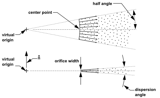
The flat-fan atomizer model is available only for 3D models. For this type of injection, you will define the following initial conditions under Point Properties:
arc position
Set the coordinates of the center point of the arc from which the fan originates in the X-Center, Y-Center, and Z-Center fields (see Figure 24.23: Flat Fan Viewed from Above and from the Side).
virtual position
Set the coordinates of the virtual origin of the fan in the X-Virtual Origin, Y-Virtual Origin, and Z-Virtual Origin fields. This point is the intersection of the lines that mark the sides of the fan (see Figure 24.23: Flat Fan Viewed from Above and from the Side).
normal vector
Set the direction that is normal to the fan in the X-Fan Normal Vector, Y-Fan Normal Vector, and Z-Fan Normal Vector fields.
temperature
Set the temperature of the streams in the Temperature field.
mass flow rate
Set the mass flow rate for the streams in the atomizer in the Flow Rate field.
duration of injection
For unsteady particle tracking (see Steady/Transient Treatment of Particles), set the starting and ending time for the injection in the Start Time and Stop Time fields. When In-Cylinder mesh motion is enabled, set the starting and ending crank angles for the injection in the Start Crank Angle and Stop Crank Angle fields.
spray half angle
Set the initial half angle of the drops as they leave the end of the orifice in the Spray Half Angle field.
orifice width
Set the width of the orifice (in the normal direction) in the Orifice Width field.
sheet breakup
Set the value of the empirical constant that determines the length of the ligaments that are formed after sheet breakup in the Flat Fan Sheet Constant field (see Equation 12–388 in the Theory Guide).
dispersion angle
For a smooth distribution of the droplets, the initial velocities is varied within this dispersion angle. A sketch of the Atomizer Dispersion Angle is depicted in Figure 24.23: Flat Fan Viewed from Above and from the Side.
time delay for reinjecting particles
If the injection is used only for reinjecting particles (Reinjection Only is enabled), you can specify Reinjection Time Delay. See The reinject Boundary Condition for details.
See The Flat-Fan Atomizer Model in the Theory Guide for details about how these inputs are used.
To randomly distribute the initial placement of the particles, enable Stagger Positions (default). The orifice width is used as radius to define the region over which particle release points will be staggered in space. For more information on spatial staggering, see Staggering of Particles in Space and Time.
For an effervescent atomizer injection, you will specify some of the same properties as for a plain-orifice atomizer. In addition to the position, axis (if 3D), temperature, mass flow rate (including both flashing and non-flashing components), duration of injection (if unsteady), vapor pressure, injector inner diameter, and azimuthal angles (if relevant) described in Point Properties for Plain-Orifice Atomizer Injections, you will need to specify the following parameters under Point Properties:
mixture quality
Set the mass fraction of the injected mixture that vaporizes in the Mixture Quality field (
 in Equation 12–398 in the Theory Guide).
saturation temperature
Set the saturation temperature of the volatile substance in the Saturation Temp. field.
droplet dispersion
Set the parameter that controls the spatial dispersion of the droplet sizes in the Dispersion Constant field (
 in Equation 12–398 in the Theory Guide).
spray angle
Set the initial trajectory of the film as it leaves the end of the orifice in the Maximum Half Angle field.
See The Effervescent Atomizer Model in the Theory Guide for details about how these inputs are used.
File injections can operate in two different modes, depending on the format of the file:
A steady file can be used in both steady and unsteady particle tracking. See Steady File Format for details.
An unsteady file can only be used in unsteady particle tracking. See Unsteady File Format for details.
An unsteady file can be converted into a steady-state injection file as described in Data Reduction of Samples.
The injection file mode is determined by the file header:
If the file does not have any header, then it is treated as a steady file for backward compatibility reasons.
If the file contains a header of the expected format, the information in the header will determine whether the file operates in the steady or unsteady mode as further described.
Important: Using an unsteady injection file for steady particle tracking will result in an error.
The steady file for a file injection has the following form:
(( x y z u v w diameter temperature mass-flow) name )
with all of the words denoting numeric parameters in scientific floating-point notation in
SI units. All the parentheses are required, but the name is
optional.
Sample files generated during sampling of trajectories for steady particle tracking as described in Sampling of Trajectories can also be used as steady injection files since they have a similar file format.
The file can have an optional two-line header automatically generated by particle sampling for steady particle tracking in the following form:
(z=4 12)
( x  y  z  u  v  w  diameter  t  mass-flow  mass  frequency  time  name)
In the first line, you can replace z=4 with an arbitrary label
that must not contain any white-space characters. You must not change the rest of the header,
but you can add any number of white space characters between its elements.
If the steady file is used in unsteady particle tracking, for every line entry in the file, a new particle parcel is generated for every injection time step in the usual way. By default, injection time steps are identical to the global fluid-flow time steps; however, you can change it in the Discrete Phase Model dialog box.
Note: The information in columns 10 and 11 (mass and
frequency) are not used for generating particles. They are only used
in a check for consistency with the particle mass specified in column 9. No check for
consistency will be made for the particle mass in relation to the particle diameter (column
7). The consistency check can be suppressed by setting the values in columns 10 and 11 to zero
The unsteady file must have a two-line header of the following format:
(z=4 13)
( x  y  z  u  v  w  diameter  t  parcel-mass  mass  n-in-parcel  time  flow-time  name)
In the first line, you can replace z=4 with an arbitrary label
that must not contain any white-space characters. You must not change the rest of the header,
but you can add any number of white space characters between its elements. The header is
automatically written by Ansys Fluent into every sampling file for unsteady particle
tracking.
The unsteady file for a file injection has the following form:
(( x y z u v w diameter temperature parcel-mass mass n-in-parcel time flow-time) name)
Here, every line entry in the file contains a time stamp
(flow-time in column 13). At the appropriate simulated
flow-time, Ansys Fluent will inject a single particle parcel only once.
That means that during the entire time interval that it spans, an unsteady injection file
produces as many particle parcels as the number of the data line entries in the file.
Like for the steady file format, all the numbers must be in SI units, and all the
parentheses are required, but the name is optional. A file that
Ansys Fluent writes from unsteady particle tracking can be used as an injection file in the
unsteady mode.
Note: The information in columns 10 and 11 (mass and
n-in-parcel) are not used for generating particles. They are only
used in a check for consistency with the particle mass specified in column 9. No check for
consistency will be made for the particle mass in relation to the particle diameter (column
7). The consistency check can be suppressed by setting the values in columns 10 and 11 to zero
An unsteady injection file can contain additional columns that can be processed using
a DEFINE_DPM_INJECTION_INIT UDF. For details, see
DEFINE_DPM_INJECTION_INIT
in the Fluent Customization Manual.
Note: In an unsteady injection file, all entries must be sorted strictly in ascending order of
the simulated flow-time (column 13). If you use unsteady particle
sampling in Ansys Fluent to generate such a file, you must select the Sort Sample
Files option in the Sample Trajectories dialog box.
In the Point Properties tab in the Set Injection Properties dialog box, you can specify the following injection parameters:
- Start Time
specifies the simulated time when Ansys Fluent starts to inject particles from this injection.
- Stop Time
specifies the simulated time when Ansys Fluent stops to inject particles from this injection.
- Start Flow-time in File
(optional) determines the line from which Ansys Fluent starts reading the injection file. All line entries in which
flow-time(13th column) is less than the specified value will be skipped. For remaining lines, the injection release time is determined as:Start Time +
flow-time- Start Flow-time in FileThe default value of 0 means that Ansys Fluent will read the injection file starting from the first line entry.
- Repeat Interval in File
(optional) can be used to put the unsteady injection into a time-periodic mode. Once Ansys Fluent has read the injection file for the specified time period, it rewinds the file and starts reading it again from the line from which it began. This cycling process continues until Stop Time is reached. In this way, detailed data for a small time interval can be used to approximate a steady state over longer time periods in an unsteady simulation with unsteady particle tracking. The default value of 0 means no repetition in time.
Note: For steady injection files, Start Flow-time in File and Repeat Interval in File are ignored.
For a condensate injection, you will define only the duration of the injection by setting the starting and ending time for the injection in the Start Time and Stop Time fields under the Point Properties tab in the Set Injection Properties dialog box. The duration of the injection determines the time during which film condensation will be initiated on the walls that have the Film Condensation option enabled.
For liquid sprays, a convenient representation of the droplet
size distribution is the Rosin-Rammler expression. The complete range
of sizes is divided into an adequate number of discrete intervals;
each represented by a mean diameter for which trajectory calculations
are performed. If the size distribution is of the Rosin-Rammler type,
the mass fraction of droplets of diameter greater than  is given by
 | (24–8) |
where  is the size constant and
  is the size distribution
parameter.
is the size distribution
parameter.
By default, you will define the size distribution of particles by inputting a diameter for the first and last points and using the linear equation (Equation 24–7) to vary the diameter of each particle stream in the group. When you want a different mass flow rate for each particle/droplet size, however, the linear variation may not yield the distribution you need. Your particle size distribution may be defined most easily by fitting the size distribution data to the Rosin-Rammler equation. In this approach, the complete range of particle sizes is divided into a set of discrete size ranges, each to be defined by a single stream that is part of the group. Assume, for example, that the particle size data obeys the following distribution:
Diameter Range ( m) m) | Mass Fraction in Range |
|---|---|
| 0–70 | 0.05 |
| 70–100 | 0.10 |
| 100–120 | 0.35 |
| 120–150 | 0.30 |
| 150–180 | 0.15 |
| 180–200 | 0.05 |
The Rosin-Rammler distribution function is based on the assumption
that an exponential relationship exists between the droplet diameter,  , and the mass fraction of
droplets with diameter greater than
, and the mass fraction of
droplets with diameter greater than  ,
,  :
:
 | (24–9) |
Ansys Fluent refers to the quantity  in Equation 24–9 as
the Mean Diameter and to
in Equation 24–9 as
the Mean Diameter and to  as the Spread Parameter. These parameters are specified by you (in the Set Injection Properties Dialog Box under the First
Point heading) to define the Rosin-Rammler size distribution.
To solve for these parameters, you must fit your particle size data
to the Rosin-Rammler exponential equation. To determine these inputs,
first recast the given droplet size data in terms of the Rosin-Rammler
format. For the example data provided above, this yields the following
pairs of
as the Spread Parameter. These parameters are specified by you (in the Set Injection Properties Dialog Box under the First
Point heading) to define the Rosin-Rammler size distribution.
To solve for these parameters, you must fit your particle size data
to the Rosin-Rammler exponential equation. To determine these inputs,
first recast the given droplet size data in terms of the Rosin-Rammler
format. For the example data provided above, this yields the following
pairs of  and
and  :
:
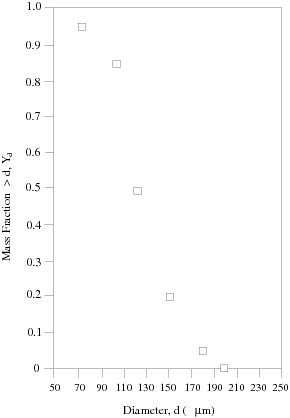
Diameter,  ( ( m) m) | Mass Fraction with Diameter Greater than
 , , 
|
|---|---|
| 70 | 0.95 |
| 100 | 0.85 |
| 120 | 0.50 |
| 150 | 0.20 |
| 180 | 0.05 |
| 200 | (0.00) |
A plot of  vs.
vs.  is shown in Figure 24.24: Example of Cumulative Size Distribution of Particles.
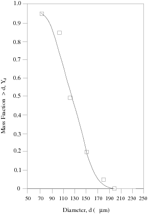
Next, derive values of  and
and  such that the data in Figure 24.24: Example of Cumulative Size Distribution of Particles fit Equation 24–9. The value for
  is obtained by noting that this is the
value of
is obtained by noting that this is the
value of  at which
  . From Figure 24.24: Example of Cumulative Size Distribution of Particles, you can estimate
that this occurs for
. From Figure 24.24: Example of Cumulative Size Distribution of Particles, you can estimate
that this occurs for  m. The numerical value for
  is given by
 | (24–10) |
By substituting the given data pairs for  and
and  into this equation, you can obtain values
for
into this equation, you can obtain values
for  and find an average. Doing so yields an average
value of
and find an average. Doing so yields an average
value of  = 4.52 for the example data above. The resulting
Rosin-Rammler curve fit is compared to the example data in Figure 24.25: Rosin-Rammler Curve Fit for the Example Particle Size Data. You can enter values for
= 4.52 for the example data above. The resulting
Rosin-Rammler curve fit is compared to the example data in Figure 24.25: Rosin-Rammler Curve Fit for the Example Particle Size Data. You can enter values for  and
and  , as well as the diameter range
of the data and the total mass flow rate for the combined individual
size ranges, using the Set Injection Properties Dialog Box.
, as well as the diameter range
of the data and the total mass flow rate for the combined individual
size ranges, using the Set Injection Properties Dialog Box.
This technique of fitting the Rosin-Rammler curve to spray data is used when reporting the Rosin-Rammler diameter and spread parameter in the Discrete Phase Summary dialog box in Summary Reporting of Current Particles.
A second Rosin-Rammler distribution is also available based
on the natural logarithm of the particle diameter. If in your case,
the smaller-diameter particles in a Rosin-Rammler distribution have
higher mass flows in comparison with the larger-diameter particles,
you may want better resolution of the smaller-diameter particle streams,
or “bins”. You can therefore choose to have the diameter
increments in the Rosin-Rammler distribution done uniformly by  .
.
In the standard Rosin-Rammler distribution, a particle injection
may have a diameter range of 1 to 200  m. In the logarithmic Rosin-Rammler
distribution, the same diameter range would be converted to a range
of
m. In the logarithmic Rosin-Rammler
distribution, the same diameter range would be converted to a range
of  to
to  , or about 0 to 5.3. In this
way, the mass flow in one bin would be less-heavily skewed as compared
to the other bins.
, or about 0 to 5.3. In this
way, the mass flow in one bin would be less-heavily skewed as compared
to the other bins.
When a Rosin-Rammler size distribution is being defined for the group of streams, you should define (in addition to the initial velocity, position, and temperature) the following parameters, which appear under the heading for the First Point:
Total Flow Rate
This is the total mass flow rate of the
 streams in the group. Note that
in axisymmetric problems this mass flow rate is defined per
streams in the group. Note that
in axisymmetric problems this mass flow rate is defined per  radians
and in 2D problems per unit meter depth.
radians
and in 2D problems per unit meter depth.Min. Diameter
This is the smallest diameter to be considered in the size distribution.
Max. Diameter
This is the largest diameter to be considered in the size distribution.
Mean Diameter
This is the size parameter,
 , in the Rosin-Rammler equation (Equation 24–9).
Spread Parameter
This is the exponential parameter,
 , in Equation 24–9.
For atomizer injections, a Rosin-Rammler distribution is assumed for the particles exiting the injector. In order to decrease the number of particles necessary to accurately describe the distribution, the diameter distribution function is randomly sampled for each instance where new particles are introduced into the domain.
The Rosin-Rammler distribution can be written as
 | (24–11) |
where  is the mass fraction smaller than a given diameter
  ,
,  is the Rosin-Rammler
diameter and
is the Rosin-Rammler
diameter and  is the Rosin-Rammler exponent. This expression can
be inverted by taking logs of both sides and rearranging,
is the Rosin-Rammler exponent. This expression can
be inverted by taking logs of both sides and rearranging,
 | (24–12) |
Given a mass fraction  along with parameters
  and
and  , this function will explicitly
provide a diameter,
, this function will explicitly
provide a diameter,  . Diameters for the atomizer injectors described
in Point Properties for Plain-Orifice Atomizer Injections are obtained
by uniformly sampling
. Diameters for the atomizer injectors described
in Point Properties for Plain-Orifice Atomizer Injections are obtained
by uniformly sampling  in Equation 24–12.
For cone, surface, and volume injections, when droplet size distribution data is available in a tabular form, you can specify the diameter distribution using a text file.
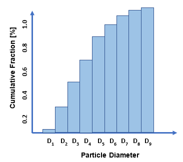
It is assumed that a measured size distribution can be approximated by a discrete number of size intervals (also called “classes”). Each class is defined by the following parameters (see Figure 24.26: Discrete Number/Mass Fraction Distribution):
Representative particle size
 ,
,Number fraction
 , and/or
Mass fraction

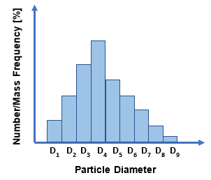
The size distribution data can also be given as a cumulative size distribution, that is, the sum of the frequency/mass distributions (see Figure 24.27: Discrete Cumulative Number/Mass Fraction Distribution).
To specify the droplet size distribution in a tabular format:
In the Set Injection Properties dialog box, select tabulated from the Diameter Distribution drop-down list.
Note: The tabulated option is available only for the cone and surface injection types.
In the Association of Particle Size Distribution Data dialog box that opens automatically, click .
Use the Table File Manager dialog box that opens to read a table file containing droplet size distribution data. See Reading Files in Tabular Format for more information on how to read table files.
Alternatively, you can read a table file as described in Reading Files in Tabular Format.
The size distribution data table is formatted as follows:
Row 1: Name of the table
Row 2: Header with the column names
Row 3 and all consecutive rows: Spray data points
The spray data points must contain the following columns separated by a space or tab delimiter:
Droplet diameter representative for an interval of the spray
The reference diameters must be sorted in either ascending or descending order.
Number fraction and/or mass fraction
Cumulative and/or non-cumulative data may be specified.
Number/mass fractions do not need to be normalized. Normalization will be performed by the solver, so that the cumulative and non-cumulative fractions are in the range of 0 to 1.
An example of the data file for the diameter size distribution data is shown below.
Dist-large
drop-diam     num-frac     mass-frac     cum-num-frac   cum-vol-frac
0.0001        0.10         1.            0.10           1
0.0002        0.2          1.            0.30           2
0.0003        0.4          1.            0.70           3
0.0004        0.4          1.            1.10           4
0.0005        0.3          1.            1.40           5
0.0006        0.28         1.            1.68           6
0.0007        0.25         1.            1.93           7
0.0008        0.22         1.            2.15           8
0.0009        0.20         1.            2.35           9
0.0010        0.15         1.            2.50           10
…
…
In this example,
Dist-largeis the name of the table. The column names are specified in the second line. The spray data points are provided starting from line 3 through the end of the file.Once the tabulated size distribution has been read into your case, the name of the table and its column names become visible and selectable in the Association of Particle Size Distribution Data dialog box. The following data will be stored in your case file:
Number of diameter classes
Representative diameters per class
Number fraction per class and/or mass fraction per class
Other injection properties (such as the number of streams to be injected and the material density)
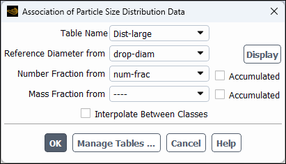
In the Association of Particle Size Distribution Data dialog box, link the size distribution parameters to the tabulated distribution data:
Select the name of your table from the Table Name drop down box.
From the Reference Diameter from, Number Fraction from, and/or Mass Fraction from drop-down lists, select the column names where the reference diameter, number fraction, and mass fraction are stored, respectively.
If the number fraction or mass fraction is available as cumulative data, select the Accumulated check box next to the corresponding variable.
Select Interpolate Between Classes if you want to generate particle diameters by linearly interpolating between neighboring diameter classes. If this option is not selected, all particles within a class will be assigned the representative class diameter.
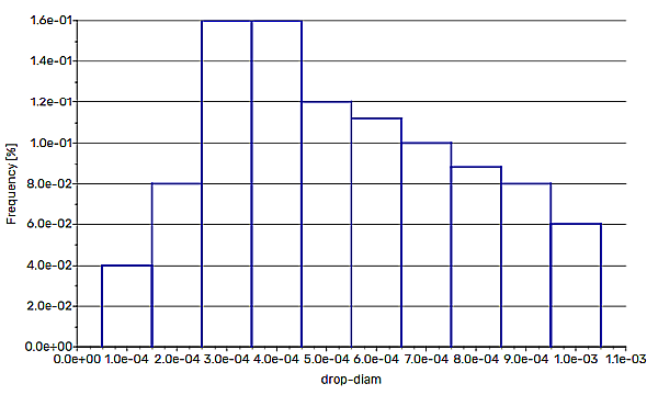
If you want to visualize the tabulated size distribution of the reference diameter over either mass fraction or number fraction, then make sure that only the column names to be used for abscissa and ordinate are selected and click Display. A histogram of the droplet size distribution data is plotted in the graphics window.
Click to close the Association of Particle Size Distribution Data dialog box.
The particle tracker first assigns particles to different diameter classes based on the supplied number fraction data. In case no number fraction data has been provided, the particle tracker derives the number-per-class information from the mass-per-class data (calculated as the mass fraction per class multiplied by the total injected mass), the material density, and the mass of the individual particle of the class.
The process of assigning a particle to a certain diameter class uses a random number generator.
For cone injections, to ensure that each class receives at least one representative particle, you must specify a sufficient number of parcels in the Number of Streams text entry field in the Set Injection Properties dialog box. As a minimum requirement, you must inject at least as many parcels as there are classes. You can obtain a rough estimate for the required number of parcels to be injected by taking the inverse of the smallest number fraction from your data. The solver, however, will tolerate empty diameter classes. The total particle mass to be injected is enforced by assigning a mass to all classes that contain at least one parcel.
For surface injections, a minimum of one parcel per surface facets will be injected.
For volume injections, you must specify a sufficient number of starting points in the number-of-starting-points or parcels-per-cell text entry field. Note that for simulations that involve DDPM, these entry fields are not available since the number of starting points is calculated automatically based on the smallest cell in the mesh. The diameter of the injected parcels is calculated so that five parcels would fit into the smallest cell volume in the mesh, while also satisfying the Injection Injection Packing Limit per Cell. If the number or the mass fraction per cell is too small to create at least one parcel in a diameter class, this class will remain empty.
Depending on the data you provide, the particle tracker uses one of the following approaches:
Only the number fraction per class is specified
In this scenario, the tracker accumulates the provided number fraction data and scales it to the range [0, 1]. This normalized data is subsequently used to assign a particle to a specific diameter class. For each particle to be injected, the tracker generates a unique random number. The number determines which size class the particle falls into. Based on the size class, the tracker sets the particle diameter. The diameter can either be either a representative diameter specified for the class or an interpolated diameter between neighboring classes to provide a more realistic spray representation.
Only the mass fraction is specified
Based on the specified mass fraction, particle material, and representative particle diameter, the approximate number of particles per class is determined. This information is used to derive the number fraction per class. Once this step is completed, the same approach is used as in the first scenario (where only the number fraction per class is specified). The tracker enforces the specified flow rate per class.
Both the number fraction and mass fraction are specified
Based on the specified number fraction data, the particle class/diameter assignment is performed as in the first scenario (where only the number fraction per class is specified). In addition, the tracker enforces the specified flow rate per class.
In cases where the number of initial particle positions is so small that the random sampling approach cannot accurately represent the diameter distribution of a spray, you can disable this approach using the following text command:
define/models/dpm/injections/properties/set/size-distribution/use-randomized-diameter-sampling?Use randomized sampling for tabulated diameter distribution? [yes]no
When this option is disabled, particles from each tabulated diameter class will be injected from each particle starting position.
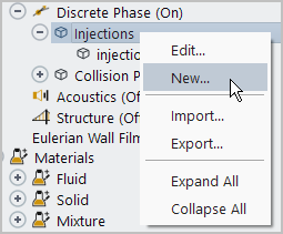
You will use the Injections branch in the Outline View and the Injections Dialog Box (Figure 24.31: The Injections Dialog Box, Figure 24.30: The Injections Branch in the Outline View ) to create, copy, delete, list, read, and write injections.
![]() Setup → Models → Discrete Phase → Injections
Setup → Models → Discrete Phase → Injections![]() New...
New...
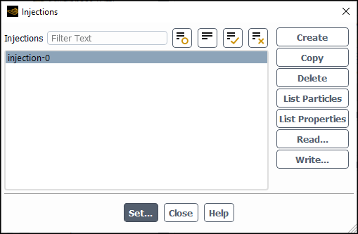
(You can also click the button in the Discrete Phase Model Dialog Box to open the Injections dialog box.)
Note: [Linux Only] If you are not part of a video group, a session on a local Linux machine with
SLES11, SP4, and OpenGL may terminate abnormally during an injection setup for the discrete
phase model case. To avoid this issue, you should restart the Ansys Fluent session with the driver
option -x11 or you should ensure that you are added to the video group
on that machine. Workaround: Deactivate the injection visualization during
the case setup by using the following scheme command:
rpsetvar 'dpm/visualize-injections? #f)
To create an injection, click the button. The Set Injection Properties Dialog Box will open automatically to allow you to set the injection properties (as described in Defining Injection Properties). After the injection is created, the new injection will appear in the Injections list, in the Injections dialog box.
To modify an existing injection, select its name in the Injections list and click the button. The Set Injection Properties dialog box will open, and you can modify the properties as needed.
If you have two or more injections for which you want to set some of the same properties, select their names in the Injections list and click the button. The Set Multiple Injection Properties dialog box will open, which will allow you to set the common properties. For instructions about using this dialog box, see Defining Properties Common to More than One Injection.
To copy an existing injection to a new injection, select the existing injection in the Injections list and click the button. The Set Injection Properties Dialog Box will open with a new injection that has the same properties as the injection you selected. This is useful if you want to set another injection with similar properties.
To list the initial conditions for the particle streams in the selected injection, click the button. Ansys Fluent reports the initial conditions (in SI units) in the console under various columns:
The particle stream number is in the column headed
NO.The particle type (
INfor inert,DRfor droplet, orCPfor combusting particle) is in the column headedTYP.The
 ,
,  , and
, and  positions are in the columns headed
 (X),(Y), and(Z).The
 ,
,  , and
, and  velocities are in the columns headed
 (U),(V), and(W).The temperature is in the column headed
(T).The diameter is in the column headed
(DIAM).The mass flow rate in the column headed
(MFLOW).
To print the properties of the selected injection(s) in the console window, click the button. Ansys Fluent reports the following basic properties for each selected injection:
General information (injection name and type, particle type and material, reference frame, and diameter distribution)
Injection point properties
Physical models
Parcel models
User laws
UDF Settings
To transfer information about DPM injections from one case file to another, use the Read... and Write... buttons. You can write selected injections to a file, which can be read into a different Ansys Fluent session, simplifying the setup of new case files. To write the injection, select the injection from the list, then click . The Select File Dialog Box will open where you can enter the name of your injection file. To read in an injection, click to open The Select File Dialog Box where you will select the injection file to read in. If the injection that you imported has the same name as that in your current case, then Ansys Fluent will rename the imported injection.
After reading injections, you may need to visit the Injections dialog box to modify the settings for the injection material and the DPM laws since the presumed settings may have changed in the current case file setup.
Once you have created an injection (using the Injections Dialog Box, as described in Creating and Modifying Injections), you will use the Set Injection Properties Dialog Box (Figure 24.32: The Set Injection Properties Dialog Box) to define the injection properties. (Remember that this dialog box will open when you create a new injection, or when you select an existing injection and click the button in the Injections dialog box.)
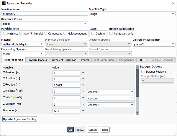
The procedure for defining an injection is as follows:
If you want to change the default name of the injection, enter a new name in the Injection Name field. This is recommended if you are defining a large number of injections so you can easily distinguish them. When assigning names to your injections, keep in mind the selection shortcut described in Creating and Modifying Injections.
Choose the type of injection in the Injection Type drop-down list. The injection choices (single, group, cone, surface, volume, plain-orifice-atomizer, pressure-swirl-atomizer, air-blast-atomizer, flat-fan-atomizer, effervescent-atomizer, condensate, and file) are described in Injection Types. Note that if you select any of the atomizer models, you also must set the Viscosity and Droplet Surface Tension in the Create/Edit Materials dialog box.
Important: Note that only surface injections from boundary surfaces will be moved with the mesh when a sliding mesh or a moving or deforming mesh is being used.
If you are using a group, cone, or any of the atomizer injections, set the Number of Streams in the group, spray cone, or atomizer.
If you are defining a surface injection, configure the following settings (see Figure 24.33: Setting Surface Injection Properties):
Choose the surface(s) from which the particles will be released in the Injection Surfaces list. Note that for surface injections that use the Randomize Starting Points option, you can only select boundary surfaces. Surfaces created in Ansys Fluent, such as iso-surfaces, rake surfaces, and so on, cannot be used.
By default, particles will be injected from the face center.
If an arbitrary number of particles should be injected from positions distributed randomly over the selected boundary surfaces, select the Randomize Starting Points option (Surface Options group box).
Note: The Randomize Starting Points and Scale Flow Rate by Face Area options are not compatible because not every surface face will be assigned exactly one starting stream when the random distribution is used. When either one of these options is selected, the other becomes unavailable.
Specify the Number of Streams (to the right of the Injection Type drop-down list) in the surface injection.
If you are defining a volume injection, configure the following settings:
From the Release From drop-down list, select how you want to define the particle release region. The following options are available:
zone
bounding-geometry
If you have chosen the zone specification method, select a suitable fluid zone(s) from which the particles will be released in the Zones selection list.
If you have chosen the bounding-geometry specification method, select an appropriate geometry to model the injection region from the Bounding Shape drop-down list:
sphere
cylinder
cone
hexahedron
and specify the Shape Coordinates. The inputs are as follows:
To define a sphere, enter the values for the Radius and the coordinates of its center: X Center, Y Center, and Z Center.
To define a cylinder, enter the value for the Radius and the minimum and maximum coordinates defining the cylinder axis: (X-Axis Min, Y-Axis Min, Z-Axis Min) and (X-Axis Max, Y-Axis Max, Z-Axis Max).
To define a cone, enter the value for the Cone Angle, the coordinates of the cone apex (X-Axis Min, Y-Axis Min, Z-Axis Min), and the coordinates of a point on the cone axis (X-Axis Max, Y-Axis Max, Z-Axis Max).
To define a hexahedron, enter the coordinates of two points defining the diagonal of the box: (X Min, Y Min, Z Min) and (X Max, Y Max, Z Max).
Select the Parcel Specification from the following options:
number-of-starting-points
parcels-per-cell (zone release region only)
and enter a value for the selected specification.
For the number-of-starting-points parcel specification, parcels will be injected into cells at uniformly distributed random points. The specified value determines the number of the starting points.
For the parcels-per-cell parcel specification, the specified value determines the number of starting points of parcels to be injected into each cell of the specified particle release region.
The Parcel Specification drop-down list is not available for DDPM cases with the Discrete Phase Domain setting other than none.
Note: For cases that involve the DDPM with the Discrete Phase Domain set to anything other than none, the number of starting points is calculated automatically based on the smallest cell in the mesh as follows. The diameter of the injected parcels is calculated so that five parcels would fit into the smallest cell volume in the mesh, while satisfying the Injection Packing Limit per Cell. The parcel volume is computed based on the parcel diameter (this is not fully applicable to 2D cases because of the special consideration stated in the Note in Steady/Transient Treatment of Particles). Then as many parcels are injected as the zone(s) or the bounding geometry can accommodate, while also respecting the Injection Packing Limit per Cell.
For DDPM simulations with the Discrete Phase Domain set to anything other than none, enter a value for Injection Packing Limit per Cell, which is the highest particle volume fraction that is possible in a computational cell.
Once the Injection Packing Limit per Cell is reached, the cells will stop receiving injected parcels, and the parcel mass will be lost. By default, Injection Packing Limit per Cell is set to the theoretical value for monodispersed solid particles of 0.63. If parcels are larger than the cells, no parcels will be injected since the Injection Injection Packing Limit per Cell would be exceeded. In DDPM simulations, a full loading or overloading of the fluid cells by setting this value to 1 or greater is not recommended as it will lead to convergence issues or potential application crashes.
You can obtain an estimation of the expected parameters for the injected particle parcels by clicking the button in the Estimated Particle Parcels group box. The following values will be reported:
Number of Particle Parcels
Total Mass
Parcel Diameter
Parcel Volume
Minimum Cell Volume in Mesh
Averaged Volume Fraction
By default, injection point properties are specified in the global reference frame/coordinate system. If you want to specify the injection point properties in one of the local reference frames that you created earlier, select that frame from the Reference Frame drop-down list. This item is not available for surface, volume, and condensate injections.
If you are reading the injection from a file, click the button at the bottom of the Set Injection Properties Dialog Box and specify the file to be read in the resulting Select File dialog box. The parameters in the injection file must be in SI units.
As the Particle Type, select one of the following:
Massless
Inert
Droplet
Combusting
Multicomponent
The available types are described in Particle Types. Note that for the condensate injection, the only available particle types are Droplet and Multicomponent.
(unsteady particle tracking only) If you are using this injection only for reinjecting particles as described in The reinject Boundary Condition, select Reinjection Only (Particle Reinjection group box).
Choose the material for the particle(s) in the Material drop-down list.
If this is the first time you have created a particle of this type, you can choose from all of the materials of this type defined in the database. If you have already created a particle of this type, the only available material will be the material you selected for that particle. You can define additional materials by copying them from the database or creating them from scratch, as discussed in Setting Discrete-Phase Physical Properties and described in detail in Using the Create/Edit Materials Dialog Box.
Important: Note that you will not choose a Material for a Massless particle type.
If you are defining a group, cone, surface, or volume injection and you want to change the default linear (group injection) or uniform (cone, surface, or volume injection) interpolation method for determining the size of the particles, you can select from the following methods in the Diameter Distribution drop-down list:
rosin-rammler
rosin-rammler-logarithmic.
tabulated (cone, surface or volume injections only)
For more information about these methods, see Using the Rosin-Rammler Diameter Distribution Method and Using the Tabulated (Discrete) Diameter Distribution.
If you have created a customized particle law using user-defined functions, enable the Custom option under Laws and specify the appropriate laws as described in Custom Particle Laws.
If you are defining Droplet particles, select the gas phase species created by the vaporization and boiling laws (Laws 2 and 3) in the Evaporating Species drop-down list.
If you are defining Combusting particles, configure the following settings:
From the Devolatilizing Species drop-down list, select the gas phase species created by the devolatilization law (Law 4).
From the Oxidizing Species drop-down list, select the gas phase species that participates in the surface char combustion reaction (Law 5).
From the Product Species drop-down list, select the gas phase species created by the surface char combustion reaction (Law 5).
Note that if the Combustion Model for the selected combusting particle material (in the Create/Edit Materials dialog box) is the multiple-surface-reaction model, then the Oxidizing Species and Product Species lists will be disabled because the reaction stoichiometry has been defined in the mixture material.
In the Point Properties tab, specify the point properties (position, velocity, diameter, temperature, and—if appropriate—mass flow rate and any atomizer-related parameters) as described for each injection type in the following sections:
If you want to set up injection-specific physics models such as drag laws, Brownian motion, and breakup, click the Physical Models tab and configure the injection physics models as described in Specifying Injection-Specific Physical Models.
If the flow is turbulent and you want to include the effects of turbulence on the particle dispersion, click the Turbulent Dispersion tab, enable the Discrete Random Walk Model under Stochastic tracking, and set the related parameters as described in Specifying Turbulent Dispersion of Particles.
If you have enabled Unsteady Particle Tracking, you can define settings for how the parcels are released. In the Parcel tab, select a Parcel Release Method from the drop-down list. The default method is standard, in which a single parcel is released per injection stream per time step. Alternatively can choose constant-number, constant-mass, or constant-diameter. Refer to Steady/Transient Treatment of Particles for details of these methods.
Note: For cases that involve the DDPM with the Discrete Phase Domain setting other than none, Ansys Fluent uses the constant-diameter parcel release method, and the Parcel tab is not available.
If your combusting particle includes an evaporating material, click the Wet Combustion tab, select the Wet Combustion Model option, and then select the material that is evaporating/boiling from the particle before devolatilization begins in the Liquid Material drop-down list. You should also set the volume fraction of the liquid present in the particle by entering the value of the Liquid Fraction. Finally, select the gas phase species created by the evaporating and boiling laws in the Evaporating Species drop-down list in the top part of the dialog box.
(Multicomponent particle type only) In the Components tab, configure the following Multicomponent Settings:
Specify the Mass Fraction of each of the components.
Note that the sum of the mass fractions should add up to unity, otherwise Ansys Fluent will scale the values such that you have a sum of 1 for the mass fraction, and will prompt you to accept the scaled values.
For each component, you have the following modeling options:
To model a species that will be vaporized, select the name of that species from the Evaporating Species drop-down list.
To model any immiscible non-volatile residue, liquid, or solid component, select none from the Evaporating Species drop-down list.
To model a non-volatile liquid component that forms a mixture with the other liquid components in the particle:
Select a relevant species from the Evaporating Species drop-down list.
For the non-volatile liquid component material, set the Saturation Vapor Pressure close to zero (in the Create/Edit Materials dialog box).
The liquid material defined in this way will form a mixture with the liquid components, but will not evaporate.
If you are using the non/partially-premixed combustion models specify the source stream for the evaporating component under Evaporating Stream.
To change the species of the multicomponent droplet:
In the Create/Edit Materials dialog box, either define a new droplet materials or copy appropriate droplet-particle materials from the Fluent materials database.
For the mixture material you want to modify, click Edit... next to Mixture Species (Property group box).
In the Species dialog box that opens, add the droplet materials that you have copied or defined to the Selected Species list and remove unwanted materials.
If you want to use a user-defined function to initialize the injection properties, click the UDF tab to access the UDF inputs. You can select an Initialization function under User-Defined Functions to modify injection properties at the time the particles are injected into the domain. This allows the position and/or properties of the injection to be set as a function of flow conditions. More information about user-defined functions can be found in the Fluent Customization Manual.
If you have defined more than one particle surface species, for example, carbon (C<s>) and sulfur (S<s>), you will need to specify the mass fraction of each particle surface species in the combusting particle. To do so, click the Multiple Reactions tab, and enter the Species Mass Fractions. These mass fractions refer to the combustible fraction of the combusting particle, and should sum to 1. If there is only one surface species in the mixture material, the mass fraction of that species will be set to 1, and you will not specify anything under Multiple Surface Reactions.
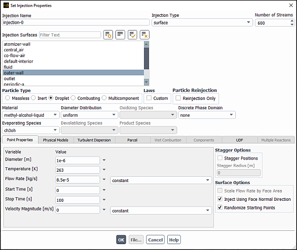
Drag and breakup models can be specified on a per-injection basis, allowing you to specify the most appropriate models for each injection in your model. These per-injection models are specified on the tab of the Set Injection Properties dialog box.
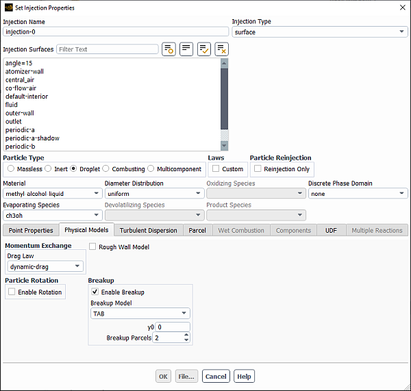
Further details are discussed in the following sections:
The following drag laws are always available:
spherical
nonspherical
Stokes-Cunningham
high-Mach-number
For more information about these models, see Particle Force Balance in the Theory Guide.
The dynamic-drag law described in Dynamic Drag Model Theory in the Theory Guide is available only when one of the droplet breakup models is used in conjunction with unsteady tracking. See Breakup for information about enabling the droplet breakup models.
The Grace and Ishii-Zuber drag laws described in Bubbly Flow Drag Laws in the Fluent Theory Guide allow to model the drag coefficient in gas-liquid flows in which the bubbles can have a range of different shapes. Both drag laws are only available if the magnitude and direction of the gravity vector are specified in the Operating Conditions dialog box.
The following drag laws:
Wen-Yu
Gidaspow
Syamlal-OBrien
Huilin-Gidaspow
Gibilaro
EMMS
Filtered
are available only when the dense discrete phase model (DDPM) is enabled (Including the Dense Discrete Phase Model) and the flow regime consists of a dense gas-solid. However, with these models, you cannot verify whether it really is a dense flow or a gas-solid flow. It is up to you to decide. In any case, these drag formulations are suitable for dense gas-solid flows.
No further inputs are required for the following drag laws:
spherical
high-Mach-number
dynamic-drag
Wen-Yu
Gidaspow
Syamlal-OBrien
Huilin-Gidaspow
Gibilaro
EMMS
Filtered
If the nonspherical law is selected, the particle Shape
Factor ( in Equation 12–52 in the Theory Guide) must be specified. The shape
factor value cannot exceed
in Equation 12–52 in the Theory Guide) must be specified. The shape
factor value cannot exceed 1.
For the Stokes-Cunningham law, the Cunningham
Correction factor ( in Equation 12–55 in the Theory Guide) must be specified.
For DPM cases with heat transfer, Ansys Fluent uses the Ranz-Marshall correlation to compute the heat transfer coefficient (see Inert Heating or Cooling (Law 1/Law 6) in the Fluent Theory Guide).
For DPM cases that include inert or combusting particles, or multicomponent particles that do not contain evaporating species, you can choose one of the following models from the Heat Transfer Coefficient drop-down list (Heat Exchange group box):
- constant-HTC
allows you to specify a constant value for the volumetric heat transfer coefficient.
- Nusselt-number
allows you to specify a value for the Nusselt number from which the heat transfer coefficient will be computed.
- Tomiyama
uses the Tomiyama model, which is suitable for turbulent bubbly flows.
- Ranz-Marshall
uses the Ranz-Marshall model described. This is the default heat transfer coefficient model for all particle types.
- Hughmark
uses the Hughmark model.
- Gunn
uses the Gunn model to compute the heat transfer coefficient. The model is applicable for flows with high volume fraction of the granular phase. This option is available only when the dense discrete phase model (DDPM) is enabled.
See Inert Heating or Cooling (Law 1/Law 6) in the Fluent Theory Guide for details about these models
Note the following:
A value of zero for constant-HTC or Nusselt-number implies that convective heat transfer is not considered.
The Heat Transfer Coefficient drop-down is available when the Energy Equation is enabled in the Energy dialog box.
To set-up particle rotation, follow the steps below:
In the Set Injection Properties dialog box, under the Physical Models tab, enable Particle Rotation.
The options related to the particle rotation feature appear in the Set Injection Properties dialog box.
From the Rotational Drag Law drop-down list, select the model for calculating the rotational drag coefficient
 . The following options are available:
- Dennis-et-al
Uses Equation 12–67 in the Fluent Theory Guide to calculate the rotational drag coefficient
 .
.- none (default)
Implies zero torque, that is, it excludes the influence of the fluid on the rotational particle motion.
From the Magnus Lift Law drop-down list, select the model for calculating the rotational lift coefficient
 . The following
models are available:
. The following
models are available:- Oesterle-Bui-Dinh
Uses Oesterle and Bui Dinh’s formulation (Equation 12–18 in the Fluent Theory Guide).
- Tsuji-et-al
Is based on the particle spin rate (Equation 12–19 in the Fluent Theory Guide).
- Rubinow-Keller
Uses a linear dependence of the rotational lift coefficient
 on the spin
rate (Equation 12–21 in the Fluent Theory Guide).
on the spin
rate (Equation 12–21 in the Fluent Theory Guide).- none (default)
Implies that the Magnus lift will not be included in your simulation.
Under the Point Properties tab, specify angular velocity components for single, group, surface, and volume injections; and angular velocity magnitudes for cone injections.
For each wall with a reflect boundary condition for the discrete phase, specify the friction coefficient (
 in Equation 12–194 and Equation 12–199 in the Fluent Theory Guide) under the DPM tab of the Wall dialog box. For details, see Friction Coefficient.
The particle rotation model options are also accessible through the text user interface, under define/models/dpm/injections/injection-properties/set/physical-models/particle-rotation. Note that the physical-models command becomes available only after you have selected the injection(s) using the prompts of the define/models/dpm/injections/properties/set/pick-injections-to-set text command.
To use the rough wall model for walls with the reflect boundary condition type:
In the Injection Settings dialog box, under the Physical Models tab, select Rough Wall Model.
In the Wall boundary conditions dialog box for the appropriate wall, under the DPM tab, select reflect from the Discrete Phase BC Type drop-down list.
Specify the following wall roughness parameters:
- Ra
is the wall mean roughness (
 in Equation 12–201 in the Fluent Theory Guide)
- Rq
is the standard deviation of the roughness structure (
 in Equation 12–201 in the Fluent Theory Guide)
- RSm
is the mean roughness slope (the average distance between peaks of wall material) (
 in Equation 12–201 in the Fluent Theory Guide)
Note: Note that the DPM Wall Roughness Parameters will only appear in the Wall dialog box with the
reflectDPM boundary condition type if the Rough Wall Model is selected in the Set Injection Properties dialog box.
For information about the rough wall model, see Rough Wall Model in the Fluent Theory Guide.
For sub-micron particles in laminar flow, you may want to include
the effects of Brownian motion (described in Brownian Force in the Theory Guide) on the
particle trajectories. To do so, enable the Brownian Motion option under the Physical Models tab. In order
to include Brownian motion effects, you must also select the Stokes-Cunningham drag law in the Drag Law drop-down list under Drag Parameters,
and specify the Cunningham Correction ( in Equation 12–55 in the Theory Guide).
This option is available only when the Energy equation is enabled (in the Models group).
To enable the modeling of particle breakup for the injection, select Enable Breakup and choose the Breakup Model (TAB, Wave, KHRT, SSD, Madabhushi or Schmehl) from the drop-down list. A detailed description of these models can be found in Secondary Breakup Model Theory in the Theory Guide.
For the TAB model, you must specify the following values:
y0: Is the initial distortion at time equal to zero (
 in Equation 12–405 in the
Theory Guide). The default value
(
in Equation 12–405 in the
Theory Guide). The default value
( ) is recommended.
 The number of Breakup Parcels: To split the droplet into several child parcels, as described in Velocity of Child Droplets in the Theory Guide. The diameter of the child parcels is sampled from a Rosin-Rammler distribution. This can be switched off in the TUI with the command:
/define/models/dpm/spray-model/tab-randomize-breakup-parcel-diameter?
For the Wave model, you must specify the following values:
B0: Is the constant
 in Equation 12–435 in the
Theory Guide.
in Equation 12–435 in the
Theory Guide. B1: Is the constant
 in Equation 12–437 in the
Theory Guide.
in Equation 12–437 in the
Theory Guide.
Note: You will generally not need to modify the value of B0, as the default value 0.61 is acceptable for nearly all cases. A value of 1.73 is recommended for B1.
The Wave model implementation has been formulated to deal with the initial breakup of a cylindrical liquid jet. In the Rayleigh regime (that is, at low gas Weber numbers), a cylindrical jet breaks up into droplets whose diameters are larger than that of the jet itself. In this regime, the model assumes that the diameter of the continuous, cylindrical liquid jet has been entered as initial diameter in the injection. Therefore, the droplet diameter can grow beyond the initial diameter. For details, see Droplet Breakup in the Fluent Theory Guide.
If you want to suppress this feature of the Wave model, use the TUI command:
/define/models/dpm/spray-model/wave-allow-rayleigh-growth? noNote that this takes effect unconditionally for all injections using the Wave or KHRT breakup models.
For the KHRT model, you must specify the following values:
B0: Is the constant
 in Equation 12–435 in the
Theory Guide.
in Equation 12–435 in the
Theory Guide.B1: Is the constant
 in Equation 12–437 in the
Theory Guide.
in Equation 12–437 in the
Theory Guide.Ctau: Is the constant
 in Equation 12–442 in the Theory Guide.
CRT: Is the constant
 in Equation 12–443 in the Theory Guide.
CL: :s the constant
 in Equation 12–438 in the
Theory Guide.
in Equation 12–438 in the
Theory Guide.
The constants B0 and B1 are the same as for the Wave model.
For the Wave model described above, the KHRT model is formulated to deal with the initial breakup of a cylindrical liquid jet. The behavior in the Rayleigh regime is as described above for the Wave model and the same TUI command can be used to modify the behavior. In addition, the model uses the Liquid Core Approximation as described in Liquid Core Length in the Fluent Theory Guide. To suppress the use of the Liquid Core Approximation you can set the Levich constant,
 , to zero.
For the SSD model, you must specify the following values:
Critical We: Is the critical Weber number in Equation 12–444 in the Theory Guide.
Core B1: Is B in Equation 12–445 in the Theory Guide.
Target Np: Is the number of droplets given to each child parcel, before scaling is used to give the correct overall mass.
Xi: Is
 in Equation 12–446 in the Theory Guide.
 Note: Xi is a negative value: exp(Xi) is a typical factor by which daughter particles are smaller than the original parcel.
For the Schmehl model, you can specify the following settings:
Breakup Parcels: Is the number of child parcels generated after splitting the droplet as described in Schmehl Breakup Model in the Fluent Theory Guide. The default is set to 1. The diameter of the child parcels is sampled from a root normal distribution described in Schmehl Breakup Model in the Fluent Theory Guide.
Breakup Max Generation: Is the maximum number of child parcel generations. The initial injected particle is considered to be generation 0, the child particles created after the first particle breakup are considered to be generation 1, and so on. When this limit is reached, the breakup process stops.
Subsequent Statistical Breakup: When enabled, the droplet breakup mechanism switches to the subsequent statistical breakup model after the Breakup Max Generation is reached. In this model no child parcels are created during the breakup mechanism. Instead, the particle number in the parcel is increased, and the particle diameter is adjusted in such a way as to conserve the full filling mass of the parent parcel.
To set up the Madabhushi breakup model, follow the steps below:
Note:For the Madabhushi breakup model, the most appropriate injection types are single, group, and cone (solid-cone). The recommended type is a solid cone injection.
The Madabhushi breakup model is available only with the dynamic-drag law (which is automatically selected from the Drag Law drop-down list when the Madabhushi breakup model is chosen) or with a drag law specified via a user-defined function (UDF). (See
DEFINE_DPM_DRAGin the Fluent Customization Manual for details.)
In the Set Injection Properties dialog box, define the Point Properties for the selected injection type (single, group, or solid cone) as follows:
Specify X-, Y-, and Z- Position in such a way that the injected droplets build a column over the midpoint of the nozzle orifice exit.
Set Diameter to the jet diameter (nozzle orifice exit diameter).
(single and group injections only) Set X-, Y-, and Z- Velocity to the inlet velocity components in x, y, and z directions, respectively.
(solid cone injections only) Set Velocity Magnitude and X-, Y-, and Z- Axis to the inlet velocity magnitude and the direction of the jet, respectively.
Set Flow Rate (single and group injections) or Total Flow Rate (solid cone injections) to the nozzle orifice flow rate.
(solid cone injections only) Set Cone angle to
0and Outer Radius to the jet radius in order to specify a perpendicular jet inflow.(solid cone injections only) In the Cone Injector Parameters group box, select Uniform Mass Distribution.
In the Physical Models tab, specify the following Madabhushi model settings.
For primary breakup based on the Wave breakup model, specify:
B0 and B1: Are the same constants as for the Wave model. The recommended values for the Madabhushi model are B0= 2.44 and B1=10. See Wave Breakup Model for details about these parameters.
Jet Diameter: Is the nozzle orifice exit diameter.
For primary breakup related to the column breakup mechanism, specify:
Ligament Factor: Adjusts the diameter of the child droplets arising from the column breakup mechanism.
C0: Is the column breakup time constant that controls how fast the column breakup occurs. The value recommended for the Madabhushi breakup model is C0=3.44.
Column Drag Cd: Is the constant drag coefficient for calculating the drag force acting on droplets within the liquid column.
To control the breakup child generation, specify Breakup Max Generation and Subsequent Statistical Breakup as described above for the Schmehl breakup model.
From the Drag Law drop-down list, select dynamic-drag.
The drag is dynamically adapted in the Madabhushi breakup model.
For more information about the Madabhushi breakup model, see Madabhushi Breakup Model in the Fluent Theory Guide.
For steady-state simulations, you also must specify an appropriate Particle Time Step Size and the Number of Time Steps, which will control the spray density. See Options for Interaction with the Continuous Phase for more information.
Note that you may want to use the dynamic drag law when you use one of the breakup models. See Drag Laws for information about choosing the drag law.
As mentioned in Defining Injection Properties, you can enable stochastic tracking for each injection to model turbulent dispersion of particles.
For turbulent flows, if you choose to use the stochastic tracking technique, you must enable the Discrete Random Walk Model and specify the Number of Tries. Stochastic tracking includes the effect of turbulent velocity fluctuations on the particle trajectories using the DRW model described in Stochastic Tracking in the Theory Guide.
Click the Turbulent Dispersion tab in the Set Injection Properties dialog box.
Enable stochastic tracking by turning on the Discrete Random Walk Model under Stochastic Tracking.
Specify the Number of Tries:
Selecting the Turbulent Dispersion model tells Ansys Fluent to include turbulent velocity fluctuations in the particle force balance as in Equation 12–22 in the Theory Guide. The trajectory is computed more than once if your input exceeds 1: two trajectory calculations are performed if you enter 2, three trajectory calculations are performed if you enter 3, and so on. Each trajectory calculation includes a new stochastic representation of the turbulent contributions to the trajectory equation.
When a sufficient number of tries is requested, the trajectories computed will include a statistical representation of the spread of the particle stream due to turbulence. Note that for unsteady particle tracking, the Number of Tries is set to 1 if using stochastic tracking.
If you want the characteristic lifetime of the eddy to be random
(Equation 12–33 in the Theory Guide), enable the Random Eddy Lifetime option. You
will generally not need to change the Time Scale Constant ( in Equation 12–24 in the Theory Guide) from its
default value of 0.15, unless you are using the Reynolds Stress turbulence
model (RSM), in which case a value of 0.3 is recommended.
in Equation 12–24 in the Theory Guide) from its
default value of 0.15, unless you are using the Reynolds Stress turbulence
model (RSM), in which case a value of 0.3 is recommended.
Figure 24.35: Mean Trajectory in a Turbulent Flow illustrates a discrete
phase trajectory calculation computed without turbulent dispersion
and Figure 24.36: Stochastic Trajectories in a Turbulent Flow illustrates the “stochastic”
tracking (number of tries  1) option.
When multiple stochastic trajectory calculations are performed, the momentum and mass defined for the injection are divided evenly among the multiple particle/droplet tracks, and are therefore spread out in terms of the interphase momentum, heat, and mass transfer calculations. Including turbulent dispersion in your model can thus have a significant impact on the effect of the particles on the continuous phase when coupled calculations are performed.
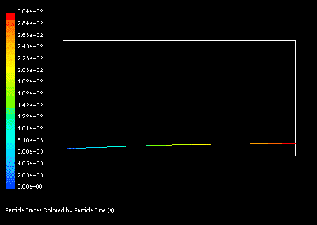
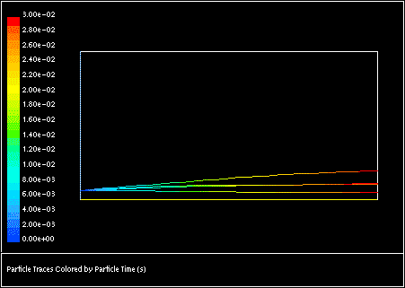
If the standard Ansys Fluent laws do not adequately describe the physics of your discrete phase model, you can modify them by creating custom laws with user-defined functions. More information about user-defined functions can be found in the Fluent Customization Manual. You can also create custom laws by using a subset of the existing Ansys Fluent laws (for example, Laws 1, 2, and 4), or a combination of existing laws and user-defined functions.
Once you have defined and loaded your user-defined function(s), you can create a custom law by enabling the Custom option under Laws in the Set Injection Properties Dialog Box. This will open the Custom Laws Dialog Box. In the drop-down list to the left of each of the particle laws, you can select the appropriate particle law for your custom law. Each list contains the available options that can be chosen (the standard laws plus any user-defined functions you have loaded).
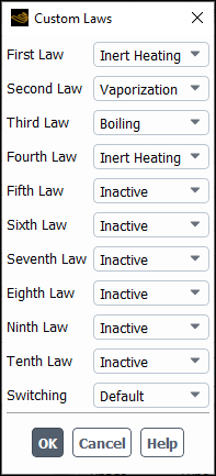
There is a final drop-down list in the Custom Laws Dialog Box labeled Switching. You may want to have Ansys Fluent vary the laws used depending
on conditions in the model. You can customize the way Ansys Fluent switches
between laws by selecting a user-defined function from this drop-down
list (see DEFINE_DPM_SWITCH in the Fluent Customization Manual).
An example of when you might want to use a custom law might be to replace the standard devolatilization law with a specialized devolatilization law that more accurately describes some unique aspects of your model. After creating and loading a user-defined function that details the physics of your devolatilization law, you would visit the Custom Laws Dialog Box and replace the standard devolatilization law (Law 2) with your user-defined function.
If you have a number of injections for which you want to set the same properties, Ansys Fluent provides a shortcut so that you do not need to visit the Set Injection Properties dialog box for each injection to make the same changes.
As described in Modifying Injections, if you select more than one injection in the Injections dialog box, clicking the button will open the Set Multiple Injection Properties dialog box (Figure 24.38: The Set Multiple Injection Properties Dialog Box) instead of the Set Injection Properties dialog box.
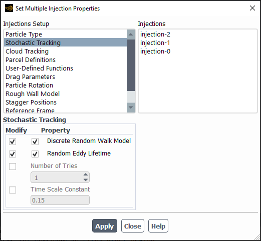
Depending on the type of injections you have selected (single, group, atomizers, and so on), there will be different categories of properties listed under Injections Setup. The names of these categories correspond to the headings within the Set Injection Properties dialog box (for example, Particle Type and Stochastic Tracking). Only those categories that are appropriate for all of your selected injections (which are shown in the Injections list) will be listed. If all of these injections are of the same type, more categories of properties will be available for you to modify. If the injections are of different types, you will have fewer categories to select from.
Note: You cannot define any properties as input parameters when you are modifying multiple injections. If you want to specify a property as an input parameter you must use Figure 24.32: The Set Injection Properties Dialog Box.
To modify a property, perform the following steps:
Select the appropriate category in the Injections Setup list. For example, if you want to set the same flow rate for all of the selected injections, select Point Properties. The dialog box will expand to show the properties that appear under that heading in the Set Injection Properties dialog box.
Set the property (or properties) to be modified, as described below.
Click . Ansys Fluent will report the change in the console window.
Important: You must click to save the property settings within each category. If, for example, you want to modify the flow rate and the stochastic tracking parameters, you will need to select Point Properties in the Injections Setup list, specify the flow rate, and click . You would then repeat the process for the stochastic tracking parameters, clicking again when you are done.
There are two types of properties that can be modified using the Set Multiple Injection Properties dialog box.
The first type involves one of the following actions:
selecting a value from a drop-down list
making a selection from a list of radio buttons
The second type involves one of the following actions:
entering a value in a field
enabling / disabling an option
Setting the first type of property works the same way as in the Set Injection Properties dialog box. For example, if you select Particle Type in the Injections Setup list, the dialog box will expand to show the portion of the Set Injection Properties dialog box where you choose the particle type. You can simply choose the desired type and click .
Setting the second type of property requires an additional step. If you select a category in the Injections Setup list that contains this type of property, the expanded portion of the dialog box will look like the corresponding part of the Set Injection Properties dialog box, with the addition of Modify check buttons (see Figure 24.38: The Set Multiple Injection Properties Dialog Box). To change one of the properties, first turn on the Modify check button to its left, and then specify the desired status or value.
For example, if you would like to enable stochastic tracking, first turn on the Modify check button to the left of Stochastic Model. This will make the property active so you can modify its status. Then, under Property, turn on the Stochastic Model check button. (Be sure to click when you are done setting stochastic tracking parameters.)
If you would like to change the value of Number of Tries, select the Modify check button to its left to make it active, and then enter the new value in the field. Make sure you click when you have finished modifying the stochastic tracking properties.
Important: The setting for a property that has not been enabled with the Modify check button is not relevant, because it will not be applied to the selected injections when you click . After you enable Modify for a particular property, clicking will modify that property for all of the selected injections, so make sure that you have the settings the way that you want them before you do this. If you make a mistake, you will have to return to the Set Injection Properties dialog box for each injection to fix the incorrect setting, if it is not possible to do so in the Set Multiple Injection Properties dialog box.
Note that it is possible to change a property that is relevant for only a subset of the selected injections. For example, if some of the selected injections are using stochastic tracking and some are not, enabling the Random Eddy Lifetime option and clicking will turn this option on only for those injections that are using stochastic tracking. The other injections will be unaffected.
Simulations of transient particles often require time dependent
injection conditions. Potentially most of the point properties may
change over time. One method to accomplish this is the use of an Initialization function as described in DEFINE_DPM_INJECTION_INIT in the Fluent Customization Manual.
An easier way is to use transient profiles containing one or more variables based on the time or crank angle that can be assigned to various point properties: (Total) Mass Flow Rate, X-, Y-, Z- Velocity, Velocity Magnitude, and Cone Angle depending on the injection type selected. See Point Properties for Single Injections to Point Properties for Effervescent Atomizer Injections for the description of the individual properties.
Before transient profile variables can be assigned to point
properties of injections, a profile file has to be read into Ansys Fluent using
the File/Read/Profile... ribbon tab item. In the Select File dialog box a transient profile in tabular format
with extension .ttab has to be chosen. Alternatively,
you can read this file into Ansys Fluent using the read-transient-table text command.
file → read-transient-table
The profile name should not exceed 63 characters. See Transient Cell Zone and Boundary Conditions for the format description. The following example illustrates an injection within 3 intervals of 2.5 milliseconds injection time, where the second injection has an elevated velocity.
mv-profile 3 13 0
time         mass-flow    velocity
0            0            0.1
0.00999      0            0.1
0.01         0.001        0.1
0.0125       0.001        0.1
0.01251      0            0.1
0.01999      0            0.1
0.02         0.001        5
0.0225       0.001        5
0.02251      0            0.1
0.02999      0            0.1
0.03         0.001        0.1
0.0325       0.001        0.1
0.03251      0            0.1
For the setting of point properties go to the Point Properties tab in the Set Injection Properties dialog box.
When transient profiles are loaded, you can choose either a constant method (the default) or profile from the Method drop-down list. If you select profile, you also must choose a profile from the corresponding drop-down list that appears in the Value column. The variable angle or time from the file is used as an independent interpolation variable and cannot be chosen as a profile.
Important: All quantities in the profile file, including coordinate values, must be specified in SI units. Specifically, Mass Flow Rate must be specified in kg/s, Velocity in m/s, and Cone Angle in radians. Ansys Fluent does not perform unit conversion when reading profile files.