


Information about mesh partitioning and load balancing is provided in the following sections:
- 43.5.1. Overview of Mesh Partitioning
- 43.5.2. Partitioning the Mesh Automatically
- 43.5.3. Partitioning the Mesh Manually and Balancing the Load
- 43.5.4. Using the Partitioning and Load Balancing Dialog Box
- 43.5.5. Mesh Partitioning Methods
- 43.5.6. Checking the Partitions
- 43.5.7. Load Distribution
- 43.5.8. Troubleshooting
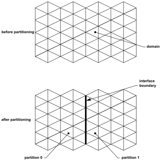
When you use the parallel solver in Ansys Fluent, you must partition or subdivide the mesh into groups of cells that can be solved on separate processors (see Figure 43.5: Partitioning the Mesh). You can either use the automatic partitioning algorithms when reading an unpartitioned mesh into the parallel solver (recommended approach, described in Partitioning the Mesh Automatically), or perform the partitioning yourself in the serial solver or after reading a mesh into the parallel solver (as described in Partitioning the Mesh Manually and Balancing the Load). In either case, the available partitioning methods are those described in Mesh Partitioning Methods. You can partition the mesh before or after you set up the problem (by defining models, boundary conditions, and so on).
Note that the relative distribution of cells among compute nodes will be maintained during mesh adaption, so manual repartitioning after adaption is not required. For details, see Load Distribution.
If you use the serial solver to set up the problem before partitioning, the machine on which you perform this task must have enough memory to read in the mesh. If your mesh is too large to be read into the serial solver, you can read the unpartitioned mesh directly into the parallel solver (using the memory available in all the defined hosts) and have it automatically partitioned. In this case you will set up the problem after an initial partition has been made. You will then be able to manually repartition the case if necessary. See Partitioning the Mesh Automatically and Partitioning the Mesh Manually and Balancing the Load for additional details and limitations, and Checking the Partitions for details about checking the partitions.
Note: When you create a Fluent mesh in parallel and read it into the Fluent solver, any partitions set up in meshing mode are preserved when the number of nodes is the same between meshing and solution modes. Performance is impacted, however, when the mesh is not balanced in Fluent meshing (as in the case of tetrahedral and prism cells).
For improved computational efficiency, automatic repartitioning occurs for any imbalanced Fluent (tetrahedral and prism) mesh when it is read into the Fluent solver. This happens regardless of any differences in the parallel node distribution of the mesh. In other words, upon being read into the Fluent parallel solver, an imbalanced parallel tetrahedral or prism mesh created in the Fluent mesher will be automatically repartitioned.
For automatic mesh partitioning, you can select the partition method and other options for creating the mesh partitions before reading a case file into the parallel version of the solver. For some of the methods, you can perform pretesting to ensure that the best possible partition is performed. See Mesh Partitioning Methods for information about the partitioning methods available in Ansys Fluent.
Note: Architecturally aware partitioning (see Partitioning) is performed automatically when the case file is read. If the maximum inter-machine communication is reduced by more than 5%, the new partition mapping will be applied, and a message is displayed in the console, for example:
inter-node communication reduction by architecture-aware
remapping: 47%
While the message indicates actual point-to-point network traffic reduction, solver computational performance improvement may be somewhat less, and depends on the case and the system network configuration.
The procedure for partitioning automatically in the parallel solver is as follows:
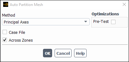
(optional) Set the partitioning parameters in the Auto Partition Mesh dialog box (Figure 43.6: The Auto Partition Mesh Dialog Box).
 Parallel → General
→ Auto Partition...
Parallel → General
→ Auto Partition... If you are reading in a mesh file or a case file for which no partition information is available, and you keep the Case File option turned on, Ansys Fluent will partition the mesh using the method displayed in the Method drop-down list. By default, the Metis method is used; as part of this method, the Laplace smoothing method is enabled by default so that adjacent highly-stretched cells are grouped together, which can significantly improve convergence and scalability. Such Laplace smoothing is controlled through preferences, as described in Preferences for Advanced Auto-Partitioning Methods.
If you want to specify the partitioning method and associated options yourself, the procedure is as follows:
Turn off the Case File option. The other options in the dialog box will become available.
Select the partition method in the Method drop-down list. The choices are the techniques described in Partition Methods.
You can choose to independently apply partitioning to each cell zone, or you can allow partitions to cross zone boundaries using the check button (which is enabled by default). It is recommended that you leave this option enabled, as otherwise the resulting partitions may be too granularized, which can compromise performance. Note that disabling this option has no effect when you have selected Metis for the Method.
If you have chosen the Principal Axes or Cartesian Axes method, you can improve the partitioning by enabling the automatic testing of the different bisection directions before the actual partitioning occurs. To use pretesting, turn on the Pre-Test option. Pretesting is described in Pretesting.
Click .
If you have a case file where you have already partitioned the mesh, and the number of partitions divides evenly into the number of compute nodes, you can keep the default selection of Case File in the Auto Partition Mesh dialog box. This instructs Ansys Fluent to use the partitions in the case file.
Read the case file.
File → Read → Case...
If you want auto-partitioning to prioritize convergence and scalability during solution, you can select a Laplace smoothing option from the Advanced Partitioning Method For Better Convergence drop-down list in the General branch of the Preferences dialog box (accessed through File/Preferences...). Through these options, the Laplace smoothing method is enabled so that adjacent highly-stretched cells are grouped together in order to prevent partition boundaries from passing through areas of high-aspect-ratio cells. There are two options:
Laplace Auto-Partition
For a case written using release 2023 R2 or later, you can select this option with the Metis auto-partition method, and Laplace smoothing will be directly based on the cell group information written into the case file. This option is selected by default with the Metis method.
Laplace Auto-Repartition
For a case written using a release previous to 2023 R2, you can select this option, so that the cell group information is created during the repartition and migration steps that take place after the auto-partitioning when reading a case file. This option can be used with any auto-partition method.
As the mesh is automatically partitioned, some information about the partitioning process will be displayed in the console. If you want additional information, you can display a report from the Partitioning and Load Balancing dialog box after the partitioning is completed.
![]() Parallel → General → Partition/Load Balance...
Parallel → General → Partition/Load Balance...
When you click the or button in the Partitioning and Load Balancing dialog box, Ansys Fluent will display the partition ID, number of cells, faces, and interfaces, and the ratio of interfaces to faces for each active or stored partition in the console. In addition, it will display the minimum and maximum cell, face, interface, and face-ratio variations. For details, see Interpreting Partition Statistics. You can examine the partitions graphically by following the directions in Checking the Partitions.
Automatic partitioning in the parallel solver (described in Partitioning the Mesh Automatically) is the recommended approach to mesh partitioning, but it is also possible to partition the mesh manually in either the serial solver or the parallel solver. After automatic or manual partitioning, you will be able to inspect the partitions created (for details, see Checking the Partitions) and optionally repartition the mesh, if necessary. Again, you can do so within the serial or the parallel solver, using the Partitioning and Load Balancing dialog box. A partitioned mesh may also be used in the serial solver without any loss in performance.
The following steps are recommended for partitioning a mesh manually:
Partition the mesh using the default method (Metis). Metis will generally produce the best quality partitions for most problems and no further user intervention should be necessary. Note that the Cartesian Axes method can be a reasonable alternative with less memory overhead.
Examine the partition statistics, which are described in Interpreting Partition Statistics. Your aim is to minimize the
Maximumvalue of thePartition boundary face count ratio, while maintaining a balanced load. For a given mesh, theMean cell count deviationis a measure of the maximum load imbalance for a method. If the statistics are not satisfactory for a problem, you can try one of the other partitioning methods.
Instructions for manual partitioning are provided below.
In order to partition the mesh, you must select the partition method for creating the mesh partitions, set the number of partitions, select the zones and/or registers, and choose the optimizations to be used. For some methods, you can also perform pretesting to ensure that the best possible partition is performed. Once you have set all the parameters in the Partitioning and Load Balancing dialog box to your satisfaction, click the button to subdivide the mesh into the selected number of partitions using the prescribed method and optimization(s). For recommended partitioning strategies see Guidelines for Partitioning the Mesh.
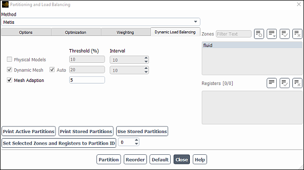
You can set the relevant inputs in the Partitioning and Load Balancing dialog box (Figure 43.7: The Partitioning and Load Balancing Dialog Box) in the following manner:
![]() Parallel → General → Partition/Load Balance...
Parallel → General → Partition/Load Balance...
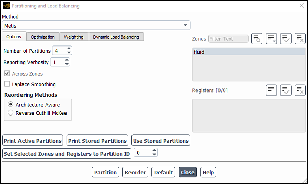
Select the Method from the drop-down list. The choices are described in Partition Methods.
In the Options tab
Set the desired number of mesh partitions in the Number of Partitions field. You can use the counter arrows to increase or decrease the value, instead of typing in the box. The number of mesh partitions must be an integer number that is divisible by the number of processors available for parallel computing.
Set the Reporting Verbosity. This allows you to control what is displayed in the console. For details, see Reporting During Partitioning.
You can choose to independently apply partitioning to each cell zone, or you can allow partitions to cross zone boundaries using the check button (which is enabled by default). It is recommended that you leave this option enabled, as otherwise the resulting partitions may be too granularized, which can compromise performance. Note that disabling this option has no effect when you have selected Metis for the Method.
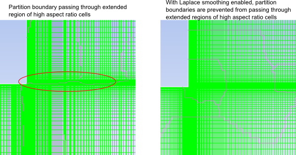
If you are using the Metis method, you have the option of enabling Laplace Smoothing. This option can be used to prevent partition boundaries from passing through areas of high aspect ratio cells. This can improve the convergence and scalability of the flow and conjugate heat transfer computations for cases with regions of highly stretched cells. After enabling Laplace Smoothing, you can specify the Cutoff Aspect Ratio. The Cutoff Aspect Ratio corresponds roughly to the maximum aspect ratio allowable along a partition boundary.
Select the Reordering Method for partitions to optimize parallel performance:
Architecture Aware: This is the default option and it accounts for the system architecture and network topology in remapping the partitions to the processors.
Reverse Cuthill-McKee: This option minimizes the bandwidth of the compute-node connectivity matrix (the maximum distance between two connected processes) without incorporating the system architecture.
The reordering methods are parallel performance tuning options. After the case is initially partitioned for parallel processing, the partition reordering step will remap the partitions in a more optimal way to improve parallel performance.
Important: The Architecture-aware reordering method is not applicable when only a single machine is used for the simulation.
After initially loading the case into a parallel session, you can click the button to reorder the partitions. The necessary algorithms are executed and Ansys Fluent will report if it can find a more optimal mapping for the partitions, as well as the potential improvement in inter-machine communications. If the reported improvement is significant (say, more than 5%), then you can click the button to use the new partition mapping. This will generally entail large data transfers amongst all the processes, and another reliable method to use the new partitions would be to write out a case file and load it back in to a new parallel session. The process is similar to re-partitioning with a new partitioning method, for example. Note that sometimes, depending on the cluster configuration and initial case partitioning, and if the partitions have already been reordered, no improvement is possible, and this will be reported in the console after clicking the button. You can simply continue in this case, and there will be no effect on the simulation. Also, note that partition reordering is specific to the current parallel configuration and should be repeated if the number of machines used changes during subsequent computations.
In the Optimization tab
You can enable and control the desired optimization methods (described in Optimizations). You can enable the Merge and Smooth schemes by enabling the check button next to each one. For each scheme, you can also set the number of Iterations. Each optimization scheme will be applied until appropriate criteria are met, or the maximum number of iterations has been executed. If the Iterations counter is set to 0, the optimization scheme will be applied until completion, with no limit on maximum number of iterations.
Choosing the Principal Axes or Cartesian Axes method, you can improve the partitioning by enabling the automatic testing of the different bisection directions before the actual partitioning occurs. To use pretesting, enable the Pre-Test option. Pretesting is described in Pretesting.
In the Zones and/or Registers lists, select the zone(s) and/or register(s) for which you want to partition. For most cases, you will select all Zones (the default) to partition the entire domain. See below for details.
You can assign selected Zones and/or Registers to a specific partition ID by entering a value for the Set Selected Zones and Registers to Partition ID. For example, if the Number of partitions for your mesh is
2, then you can only use IDs of0or1. If you have three partitions, then you can enter IDs of0,1, or2. This can be useful in situations where the gradient at a region is known to be high. In such cases, you can mark the region or zone and set the marked cells to one of the partition IDs, thereby preventing the partition from going through that region. This in turn will facilitate convergence. This is also useful in cases where mesh manipulation tools are not available in parallel. In this case, you can assign the related cells to a particular ID so that the mesh manipulation tools are now functional.If you are running the parallel solver, and you have marked your region and assigned an ID to the selected Zones and/or Registers, click the button to make the new partitions valid.
Refer to the example described later in this section for a demonstration of how selected registers are assigned to a partition (Example of Setting Selected Cell Registers to Specified Partition IDs).
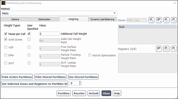
In the Weighting tab (Figure 43.8: The Weighting Tab in the Partitioning and Load Balancing Dialog Box), you can set the appropriate weights prior to partitioning the mesh, to improve load balancing and overall performance. You can control weights for cells, solid cell zones, VOF, DPM, and ISAT table lookup. You can rely on Ansys Fluent timers to set the weight scaling and optionally modify it (by enabling the User Specified option); alternatively, you can use model-weighted partitioning, so that Fluent automatically calculates the weighting based on the cell count and the models and attributes used as weights.
Enable Faces per Cell so that the partitioning assigns a weight to each cell based on its number of faces. This type of weighting is advantageous when the case has mixed or polyhedral cell zones. If you enable the User Specified check box, the weight assigned to each cell will be the number of faces plus the Additional Cell Weight you enter in the number-entry box under Value. By default the Faces per Cell weighting is enabled with the Additional Cell Weight set to 2.
Enable Solid Zones weighting so that the partitioning takes solid cells into consideration. If you enable the User Specified check box, you can specify a Value for the Solid Cell Weight Ratio. This value is relative to the fluid cell weighting; typically, it should be less than 1, since the calculation is usually quicker and less computationally expensive for the solid zone compared to the fluid zone. When using model-weighted partitioning, the default value of
0.1is appropriate, otherwise a larger value may be more suitable. For cases that have solid zones, the Solid Zones weighting is enabled by default.Note: The solid cell count must be within 30–70% of the total cell count, otherwise the model-weighted partitioning will not consider solid cells.
Enable VOF weighting to allow the partitioning to consider the imbalance caused by the free surface reconstruction with the geo-reconstruct scheme. Therefore, it is only available when using the VOF model with geometric reconstruction. You may use the user-specified value before timers are collected, or if you want to specify a value other than timing statistics. The specified value is the VOF proportion of the total computational effort.
Enable DPM weighting to set the weight of DPM particles relative to the continuous phase. DPM weights are valid when you have particle tracking in your simulation, where the user-specified value is the DPM proportion of the total computational effort relative to the continuous phase. Note that this is available only when you have injections defined. For details, see Modeling Discrete Phase.
The DPM weight takes into account the distribution of the tracking effort over the partitions and it is available after at least one calculation step with particle tracking. Displaying Particle Tracks does not change the weights. The computational effort is determined by the number of DPM steps performed in each cell. This weight becomes more important when the time for the particle tracking of particles exceeds the time for solving the flow. Enabling this option in the Weighting tab enables the counting of the particle steps in the cells. These values are available for contour and vector plots when using the Discrete Phase Model and DPM Steps per Cell variable. After repartitioning, the DPM weights are reset before the next particle tracking. It is generally preferable to partition along the dominant path of the particles in order to minimize particles crossing partition boundaries and thereby reducing associated communication costs. However, partitioning should also consider load balance for the other models, especially the continuous phase, and model weighting provides a means to effectively load balance the overall simulation.
Select the Hybrid Optimization option to enable the hybrid optimization partition weighting method for DPM. This method balances the load across machines, and, within each machine, the hybrid parallel DPM method is used to make sure the load is balanced by multi-threading. First, the domain is split based on the model weights of each cell and then partitioned across a number of machines. Finally, each machine is partitioned according to the number of cores. This allows you to have a balanced number of cells in each partition, at the same time having a balanced number of particles on each machine, which will be further balanced by the hybrid DPM method. This optimization option is also applicable to the discrete element method (DEM) collision model.
Enable ISAT weighting to balance the load during the ISAT table lookup for the stiff-chemistry Laminar, EDC or PDF Transport models. The ISAT algorithm builds an unstructured table in
 species dimensions for storage and retrieval of the chemistry
mappings. Since chemistry is usually computationally expensive, this
storage/retrieval can be very time-consuming (for information about ISAT, refer to
In-Situ Adaptive Tabulation (ISAT) in the Theory Guide). Each parallel node
builds its own table, and there is no message passing to tables on other nodes. As
some nodes may have more chemical reactions than others (for example one parallel
node may contain just air at a constant temperature, in which case the ISAT table
will contain only one entry and calculation will be rapid), there may be a load
imbalance. The dynamic load balancing algorithm will migrate cells from high
computational load nodes to low computational load nodes.
species dimensions for storage and retrieval of the chemistry
mappings. Since chemistry is usually computationally expensive, this
storage/retrieval can be very time-consuming (for information about ISAT, refer to
In-Situ Adaptive Tabulation (ISAT) in the Theory Guide). Each parallel node
builds its own table, and there is no message passing to tables on other nodes. As
some nodes may have more chemical reactions than others (for example one parallel
node may contain just air at a constant temperature, in which case the ISAT table
will contain only one entry and calculation will be rapid), there may be a load
imbalance. The dynamic load balancing algorithm will migrate cells from high
computational load nodes to low computational load nodes.If you decide to specify a value, this user-specified value is the ISAT proportion of the total computational effort.
For the Metis partition method, you have the option of using model-weighted partitioning. The objective of model-weighted partitioning is to balance the overall number of cells, as well as the time needed for the selected models (that is, the enabled Weight Types, described previously). This is specifically useful for cases that could potentially lead to a load imbalance—for example: when using the discrete phase model, as the distribution of particles could be different across partitions and thus cause an imbalance; or for cases with a large proportion of solid zones, as solid zones require less processing time / expense than fluid zones.
Each model is considered as a constraint, and a base constraint is automatically introduced for the overall number of cells. When partitioning, ANSYS Fluent will automatically calculate the weights for these constraints, and balance each of them.
To use model-weighted partitioning, ensure that the Metis partition method is selected, and enable the appropriate models under Weight Types in the Weighting tab; note that for VOF, DPM, and ISAT, the associated User Specified and Value settings are not relevant). Then make sure that the following text command is enabled (which it is by default) prior to partitioning:
parallel→partition→set→model-weighted-partitionNote that you can get additional information specific to the constraints by setting the Reporting Verbosity to 2 in the Options tab.
When using the dynamic mesh model in your parallel simulations, the Partition dialog box includes an Auto Repartition option and a Repartition Interval setting. These parallel partitioning options are provided because Ansys Fluent migrates cells when remeshing and smoothing are performed. Therefore, the partition interface becomes very wrinkled and the load balance may deteriorate. By default, the Auto Repartition option is selected, where a percentage of interface faces and loads are automatically traced. When this option is selected, Ansys Fluent automatically determines the most appropriate repartition interval based on various simulation parameters. Sometimes, using the Auto Repartition option provides insufficient results, therefore, the Repartition Interval setting can be used. The Repartition Interval setting lets you to specify the interval (in time steps or iterations respectively) when a repartition is enforced. When repartitioning is not desired, you can set the Repartition Interval to zero.
Important: Note that when dynamic meshes and remeshing is utilized, updated meshes may be slightly different in parallel Ansys Fluent (when compared to serial Ansys Fluent or when compared to a parallel solution created with a different number of compute nodes), resulting in very small differences in the solutions.
Click the button to partition the mesh.
Click the button if you decide that the new partitions are better than the previous ones (if the mesh was already partitioned). This makes the newly stored cell partitions the active cell partitions. The active cell partition is used for the current calculation, while the stored cell partition (the last partition performed) is used when you save a case file.
Start Ansys Fluent in parallel. The case in this example was partitioned across two nodes.
Read in your case.
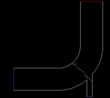
Display the mesh with the Partitions option enabled in the Mesh Display dialog box (Figure 43.9: The Partitioned Mesh).
Mark your cells using a region cell register (for details, see Region). This creates a cell register.
Open the Partitioning and Load Balancing dialog box.
Set the Set Selected Zones and Registers to Partition ID to
0and click the corresponding button. This displays the following output in the Ansys Fluent console:>> 2 Active Partitions: ---------------------------------------------------------------------- Collective Partition Statistics: Minimum Maximum Total ---------------------------------------------------------------------- Cell count 459 459 918 Mean cell count deviation 0.0% 0.0% Partition boundary cell count 11 11 22 Partition boundary cell count ratio 2.4% 2.4% 2.4% Face count 764 1714 2461 Mean face count deviation -38.3% 38.3% Partition boundary face count 13 13 17 Partition boundary face count ratio 0.8% 1.7% 0.7% Partition neighbor count 1 1 ---------------------------------------------------------------------- Partition Method Metis Stored Partition Count 2 Done.
Click the button to make the new partitions valid. This migrates the partitions to the compute-nodes. The following output is then displayed in the Ansys Fluent console:
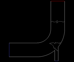
Migrating partitions to compute-nodes. >> 2 Active Partitions: P Cells I-Cells Cell Ratio Faces I-Faces Face Ratio Neighbors 0 672 24 0.036 2085 29 0.014 1 1 246 24 0.098 425 29 0.068 1 ---------------------------------------------------------------------- Collective Partition Statistics: Minimum Maximum Total ---------------------------------------------------------------------- Cell count 246 672 918 Mean cell count deviation -46.4% 46.4% Partition boundary cell count 24 24 48 Partition boundary cell count ratio 3.6% 9.8% 5.2% Face count 425 2085 2461 Mean face count deviation -66.1% 66.1% Partition boundary face count 29 29 49 Partition boundary face count ratio 1.4% 6.8% 2.0% Partition neighbor count 1 1 ---------------------------------------------------------------------- Partition Method Metis Stored Partition Count 2 Done.Display the mesh (Figure 43.10: The Partitioned ID Set to Zero).
This time, set the Set Selected Zones and Registers to Partition ID to
1and click the corresponding button. This displays a report in the Ansys Fluent console.Click the button to make the new partitions valid and to migrate the partitions to the compute-nodes.
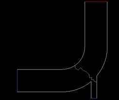
Display the mesh (Figure 43.11: The Partitioned ID Set to 1). Notice now that the partition appears in a different location as specified by your partition ID.
Important: Although this example demonstrates setting selected registers to specific partition IDs in parallel, it can be similarly applied in serial.
The ability to restrict partitioning to cell zones or registers gives you the flexibility to apply different partitioning strategies to subregions of a domain. For example, if your geometry consists of a cylindrical plenum connected to a rectangular duct, you may want to partition the plenum using the Cylindrical Axes method, and the duct using the Cartesian Axes method.
If the plenum and the duct are contained in two different cell zones, you can select one at a time and perform the desired partitioning, as described in Using the Partitioning and Load Balancing Dialog Box. If they are not in two different cell zones, you can create a cell register (basically a list of cells) for each region using the functions that are used to mark cells for adaption. These functions allow you to mark cells based on physical location, cell volume, gradient or isovalue of a particular variable, and other parameters. See Adapting the Mesh for information about marking cells for adaption. Using Cell Registers provides information about creating cell registers. Once you have created a cell register, you can partition within it as described in Example of Setting Selected Cell Registers to Specified Partition IDs.
Important: Note that partitioning within zones or registers is not available when Metis is selected as the partition Method.
For dynamic mesh applications, Ansys Fluent stores the partition method used to partition the respective zone. Therefore, if repartitioning is done, Ansys Fluent uses the same method that was used to partition the mesh.
As the mesh is partitioned, information about the partitioning process will be displayed in the console. By default, the number of partitions created, the time required for the partitioning, and the minimum and maximum cell, face, interface, and face-ratio variations will be displayed (for details, see Interpreting Partition Statistics). If you increase the Reporting Verbosity to 2 from the default value of 1, the partition method used, the partition ID, number of cells, faces, and interfaces, and the ratio of interfaces to faces for each partition will also be displayed in the console. If you decrease the Reporting Verbosity to 0, only the number of partitions created and the time required for the partitioning will be reported.
You can request a portion of this report to be displayed again after the partitioning is completed. When you click the or button in the serial or parallel solver, Ansys Fluent will display the partition ID, number of cells, faces, and interfaces, and the ratio of interfaces to faces for each active or stored partition in the console. In addition, it will display the minimum and maximum cell, face, interface, and face-ratio variations. For details, see Interpreting Partition Statistics.
Important: Recall that to make the stored cell partitions the active cell partitions you must click the button. The active cell partition is used for the current calculation, while the stored cell partition (the last partition performed) is used when you save a case file.
If you change your mind about your partition parameter settings, you can easily return to the default settings assigned by Ansys Fluent by clicking on the button. When you click the button, it will become the Reset button. The Reset button allows you to return to the most recently saved settings (that is, the values that were set before you clicked on ). After execution, the button will become the button again.
A dynamic load balancing capability is available in Ansys Fluent. The principal reason for using parallel processing is to reduce the turnaround time of your simulation, which may be achieved by the following means:
Faster machines, for example, faster CPU, memory, cache, and communication bandwidth between the CPU and memory
Faster interconnects, for example, smaller latency and larger bandwidth
Better Load balancing, for example, load is evenly distributed and CPUs are not idled during calculation
The first two evolve at the pace of computer technology, which is beyond the scope of this document. The third item is regarding optimization of available computation power. Here we are mainly talking about load balancing on dedicated homogeneous resources, which is often the case nowadays. If you are not using a dedicated homogeneous resource, you may need to account for differences in CPU speeds during partitioning by specifying a load distribution (for details, see Load Distribution).
On a dedicated homogeneous system, the key for load balancing is how to evaluate the computational requirement of each cell. By default, Ansys Fluent assumes that each cell requires the same computational work, but this is often not the case. For example
A hexahedral cell demands more CPU and memory than a tetrahedral cell.
A cell with particle tracking will use more time than a cell without particle tracking.
ISAT species model cells may have magnitude differences in time usage.
To balance these differences, ideally, the time used in each cell could be recorded and load balance achieved based on these detailed timing statistics. However, this can be expensive and such low level timings can be unreliable in any case. Instead, we identify features causing computational imbalance and record time usage for these models in aggregate. For a more detailed description of this, refer to Partitioning in the discussion of the Weighting tab. In addition, the imbalance may happen dynamically during run time, for example
The mesh may be changed by adaption or mesh movement.
In unsteady cases, particle tracking may move from one region to another region.
Dynamic load balancing has been implemented for better scalability of cases with imbalanced physical or geometrical models, thereby reducing the simulation time. The implementation considers weights from these models scaled by CPU time usage. Load balancing for DPM, VOF, cell type (number of faces per cell), and solid zones can be performed. In addition, cell weight based load balancing and machine load distribution can also be specified (for details, see Load Distribution). Ansys Fluent takes the weights from physical models and considers them for partitioning. The weights are assembled based on the time used by each physical model. For dynamic load balancing, the load is checked and balanced based on your specified imbalance threshold. To apply dynamic load balancing on the various models, click the Dynamic Load Balancing tab and select the required balancing as follows:
Enable Physical Models load balancing during iterations so that the load will be evaluated for time usage and weight distribution, based on the Interval that you provide. If the imbalance exceeds the specified Threshold, then repartitioning will be performed by considering the selected weights. Physical Models load balancing will only be available when you have the specific physical models enabled in the case. You will be prompted to enable the weights for those models. When weights for the physical models are all disabled, you will be prompted to disable Physical Models load balancing.
Note: Applying load balancing too frequently may cause performance degradation due to the additional cost of migrating cells for the new partition layout.
Enable Dynamic Mesh if there is any dynamic mesh movement. Load balancing, based on the number of cells, will be checked and balanced if the imbalance threshold is exceeded. These parallel partitioning options are provided because with mesh motion, when remeshing and smoothing are performed, the partition interface can become very wrinkled and load balance may deteriorate. By default, the Auto option is selected, where a percentage of interface faces and loads are automatically traced. When this option is selected, Ansys Fluent automatically determines the most appropriate repartitioning interval based on various simulation parameters. However, sometimes, the frequency of load balancing from the Auto option may be inadequate, and then the Interval setting can be explicitly set. The Interval setting lets you specify the interval (in time steps or iterations, respectively) when load balancing is enforced. When load balancing is not desired, you may disable Dynamic Mesh load balancing. Dynamic Mesh load balancing is only available when you have dynamic models enabled in your case.
Important: Note that when dynamic meshes and remeshing are utilized, updated meshes may be slightly different in parallel Ansys Fluent (when compared to serial Ansys Fluent or when compared to a parallel solution created with a different number of compute nodes), resulting in very small differences in the solutions.
Enable Mesh Adaption. Any time mesh adaption occurs, load balancing, based on the number of cells, will be checked and balanced if the imbalance threshold is exceeded. If problems arise in your computations due to adaption, you can disable the load balancing for Mesh Adaption.
Partitioning the mesh for parallel processing has three major goals:
Create partitions with equal numbers of cells.
Minimize the number of partition interfaces — that is, decrease partition boundary surface area.
Minimize the number of partition neighbors.
Balancing the partitions (equalizing the number of cells) ensures that each processor has an equal load and that the partitions will be ready to communicate at about the same time. Since communication between partitions can be a relatively time-consuming process, minimizing the number of interfaces can reduce the time associated with this data interchange. Minimizing the number of partition neighbors reduces the chances for network and routing contentions. In addition, minimizing partition neighbors is important on machines where the cost of initiating message passing is expensive compared to the cost of sending longer messages. This is especially true for workstations connected in a network.
The partitioning schemes in Ansys Fluent use bisection or METIS algorithms to create the partitions, but unlike other schemes that require the number of partitions to be a factor of two, these schemes have no limitations on the number of partitions. You will create as many partitions as there are computing units (cores based on processors and machines) available for your simulation.
The mesh is partitioned using a bisection or METIS algorithm. The selected algorithm is applied to the parent domain, and then recursively applied to the subdomains. For example, to divide the mesh into four partitions with a bisection method, Fluent will bisect the entire (parent) domain into two child domains, and then repeat the bisection for each of the child domains, yielding four partitions in total. To divide the mesh into three partitions with a bisection method, Fluent will "bisect" the parent domain to create two partitions—one approximately twice as large as the other—and then bisect the larger child domain again to create three partitions in total. METIS uses graph partitioning techniques that generally provide more optimal partitions than the geometric methods.
The mesh can be partitioned using one of the algorithms listed below. The most efficient choice is problem-dependent, so you can try different methods until you find the one that is best for your problem. See Guidelines for Partitioning the Mesh for recommended partitioning strategies.
- Cartesian Axes
bisects the domain based on the Cartesian coordinates of the cells (see Figure 43.13: Partitions Created with the Cartesian Axes Method). It bisects the parent domain and all subsequent child subdomains perpendicular to the coordinate direction with the longest extent of the active domain. It is often referred to as coordinate bisection.
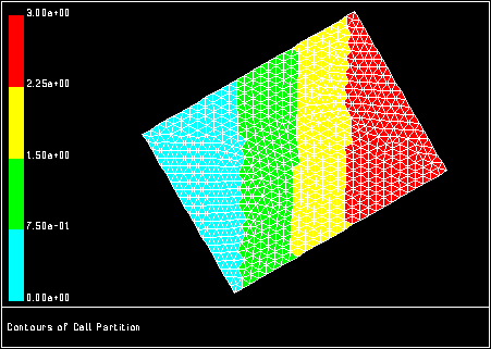
- Cartesian Strip
uses coordinate bisection but restricts all bisections to the Cartesian direction of longest extent of the parent domain (see Figure 43.14: Partitions Created with the Cartesian Strip or Cartesian X-Coordinate Method). You can often minimize the number of partition neighbors using this approach.
- Cartesian X-, Y-, Z-Coordinate
bisects the domain based on the selected Cartesian coordinate. It bisects the parent domain and all subsequent child subdomains perpendicular to the specified coordinate direction. (See Figure 43.14: Partitions Created with the Cartesian Strip or Cartesian X-Coordinate Method.)
- Cartesian R Axes
bisects the domain based on the shortest radial distance from the cell centers to that Cartesian axis (
 ,
,  , or
, or  ) whichever produces the smallest
interface size. This method is available only in 3D.
) whichever produces the smallest
interface size. This method is available only in 3D.- Cartesian RX-, RY-, RZ-Coordinate
bisects the domain based on the shortest radial distance from the cell centers to the selected Cartesian axis (
 ,
,  , or
, or  ). These methods are available
only in 3D.
). These methods are available
only in 3D.- Cylindrical Axes
bisects the domain based on the cylindrical coordinates of the cells. This method is available only in 3D.
- Cylindrical R-, Theta-, Z-Coordinate
bisects the domain based on the selected cylindrical coordinate. These methods are available only in 3D.
- Metis
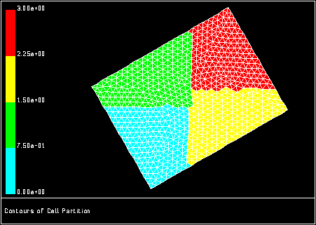
uses the METIS software package for partitioning irregular graphs, developed by Karypis and Kumar at the University of Minnesota and the Army HPC Research Center. It uses a multilevel approach in which the vertices and edges on the fine graph are coalesced to form a coarse graph. The coarse graph is partitioned, and then uncoarsened back to the original graph. During coarsening and uncoarsening, algorithms are applied to permit high-quality partitions. METIS routines can handle partitioning with model-weighted multiple constraints: when automatically partitioning, solid cell zones are weighted with a default value of 0.1 relative to the fluid cell weighting; when manually partitioning, you can control weighting for cells, solid cell zones, VOF, DPM, and ISAT table lookup (as described in Partitioning). Detailed information about METIS can be found in [75] and [76].
Important: If you create non-conformal interfaces, and generate virtual polygonal faces, your METIS partition can cross non-conformal interfaces by using the connectivity of the virtual polygonal faces. This improves load balancing for the parallel solver and minimizes communication by decreasing the number of partition interface cells.
- Polar Axes
bisects the domain based on the polar coordinates of the cells (see Figure 43.17: Partitions Created with the Polar Axes or Polar Theta-Coordinate Method). This method is available only in 2D.
- Polar R-Coordinate, Polar Theta-Coordinate
bisects the domain based on the selected polar coordinate (see Figure 43.17: Partitions Created with the Polar Axes or Polar Theta-Coordinate Method). These methods are available only in 2D.
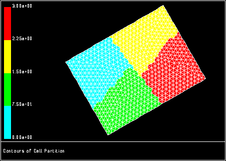
- Principal Axes
bisects the domain based on a coordinate frame aligned with the principal axes of the domain (see Figure 43.15: Partitions Created with the Principal Axes Method). This reduces to Cartesian bisection when the principal axes are aligned with the Cartesian axes. The algorithm is also referred to as moment, inertial, or moment-of-inertia partitioning.
This is the default bisection method in Ansys Fluent.
- Principal Strip
uses moment bisection but restricts all bisections to the principal axis of longest extent of the parent domain (see Figure 43.16: Partitions Created with the Principal Strip or Principal X-Coordinate Method). You can often minimize the number of partition neighbors using this approach.
- Principal X-, Y-, Z-Coordinate
bisects the domain based on the selected principal coordinate (see Figure 43.16: Partitions Created with the Principal Strip or Principal X-Coordinate Method).
- Spherical Axes
bisects the domain based on the spherical coordinates of the cells. This method is available only in 3D.
- Spherical Rho-, Theta-, Phi-Coordinate
bisects the domain based on the selected spherical coordinate. These methods are available only in 3D.
Additional optimizations can be applied to improve the quality of the mesh partitions. The heuristic of bisecting perpendicular to the direction of longest domain extent is not always the best choice for creating the smallest interface boundary. A pre-testing operation (for details, see Pretesting) can be applied to automatically choose the best direction before partitioning. In addition, the following iterative optimization schemes exist:
- Smooth
attempts to minimize the number of partition interfaces by swapping cells between partitions. The scheme traverses the partition boundary and gives cells to the neighboring partition if the interface boundary surface area is decreased. (See Figure 43.18: The Smooth Optimization Scheme.)
- Merge
attempts to eliminate orphan clusters from each partition. An orphan cluster is a group of cells with the common feature that each cell within the group has at least one face that coincides with an interface boundary. (See Figure 43.19: The Merge Optimization Scheme.) Orphan clusters can degrade multigrid performance and lead to large communication costs.


In general, the Smooth and Merge schemes are relatively inexpensive optimization tools.
If you choose the Principal Axes or Cartesian Axes method, you can improve the bisection by testing different directions before performing the actual bisection. If you choose not to use pretesting (the default), Ansys Fluent will perform the bisection perpendicular to the direction of longest domain extent.
If pretesting is enabled, it will occur automatically when you click the button in the Partitioning and Load Balancing Dialog Box, or when you read in the mesh if you are using automatic partitioning. The bisection algorithm will test all coordinate directions and choose the one which yields the fewest partition interfaces for the final bisection.
Note that using pretesting will increase the time required for partitioning. For 2D problems partitioning will take 3 times longer than without pretesting, and for 3D problems it will take 4 times longer.
As noted above, you can use the METIS partitioning method through a filter in addition to within the Auto Partition Mesh and Partitioning and Load Balancing dialog boxes. To perform METIS partitioning on an unpartitioned mesh, use the File/Import/Partition/Metis... ribbon tab item.
![]() File → Import → Partition → Metis...
File → Import → Partition → Metis...
Ansys Fluent will use the METIS partitioner to partition the mesh, and then read the partitioned mesh. The number of partitions will be equal to the number of processes. You can then proceed with the model definition and solution.
Important: Direct import to the parallel solver through the partition filter requires that the host machine has enough memory to run the filter for the specified mesh. If not, you must run the filter on a machine that does have enough memory. You can either start the parallel solver on the machine with enough memory and repeat the process described above, or run the filter manually on the new machine and then read the partitioned mesh into the parallel solver on the host machine.
To manually partition a mesh using the partition filter, enter the following command:
utility partition input_filename partition_count output_filename
where input_filename is the filename for the mesh to be partitioned, partition_count is the number of partitions desired, and output_filename is the filename for the partitioned mesh. You can then read the partitioned mesh into Fluent (using the standard File/Read/Case... ribbon tab item) and proceed with the model definition and solution.
When the File/Import/Partition/Metis... ribbon tab item is used to import an unpartitioned mesh into the parallel solver, the METIS partitioner partitions the entire mesh. You may also partition each cell zone individually, using the File/Import/Partition/Metis Zone... ribbon tab item.
![]() File → Import → Partition → Metis Zone...
File → Import → Partition → Metis Zone...
This method can be useful for balancing the work load for cases that have few cell zones.
After partitioning a mesh, you should check the partition information and examine the partitions graphically.
You can request a report to be displayed after partitioning (either automatic or manual) is completed. Click the or button in the Partitioning and Load Balancing dialog box.
Ansys Fluent distinguishes between two cell partition schemes: the active cell partitions and the stored cell partitions. Initially, both are set to the cell partitions that were established upon reading the case file. If you re-partition the mesh using the Partitioning and Load Balancing dialog box, the new partitions will be referred to as the stored cell partitions. To make them the active cell partitions, you must click the button in the Partitioning and Load Balancing dialog box in the parallel version of Ansys Fluent. The active cell partitions are used for the current calculation, while the stored cell partitions (determined from the last partitioning performed) are used when you save a case file. This distinction is made mainly to allow you to partition a case on one machine or network of machines and solve it on a different one. Thanks to the two separate partitioning schemes, you could use the parallel solver with a certain number of compute nodes to subdivide a mesh into an arbitrary different number of partitions, suitable for a different parallel machine, save the case file, and then load it into the designated machine.
The output generated when you print the partitions consists of tabulated information about the active or stored partitioning scheme. A typical output for a mesh with 4 partitions is as follows:
>> 4 Active Partitions:
P Cells I-Cells Cell Ratio Faces I-Faces Face Ratio Neighbors Load
0 3520 142 0.040 11399 195 0.017 1 1
1 3298 115 0.035 10678 151 0.014 1 1
2 3451 305 0.088 11404 372 0.033 2 1
3 3583 332 0.093 11586 416 0.036 2 1
----------------------------------------------------------------------
Collective Partition Statistics: Minimum Maximum Total
----------------------------------------------------------------------
Cell count 3298 3583 13852
Mean cell count deviation -4.8% 3.5%
Partition boundary cell count 115 332 894
Partition boundary cell count ratio 3.5% 9.3% 6.5%
Face count 10678 11586 44500
Mean face count deviation -5.2% 2.8%
Partition boundary face count 151 416 567
Partition boundary face count ratio 1.4% 3.6% 1.3%
Partition neighbor count 1 2
----------------------------------------------------------------------
Partition Method Metis
Stored Partition Count 4The first table in the output displays per-partition statistics of interest:
-
P the partition ID
-
Cells the number of cells in the partition
-
I-Cells the number of interface cells in the partition (that is, cells that lie on the partition interfaces)
-
Cell Ratio the ratio of interface cells to total cells for the partition
-
Faces the number of faces in the partition
-
I-Faces the number of interface faces in the partition (that is, faces that lie on partition interfaces)
-
Face Ratio the ratio of interface faces to total faces for the partition
-
Neighbors the number of neighbor partitions
-
Load the desired relative load on this node in proportion to the other nodes. See Load Distribution for details.
Note that partition IDs correspond directly to compute node IDs when a case file is
read into the parallel solver. When the number of partitions in a case file is larger than
the number of compute nodes, but is evenly divisible by the number of compute nodes, then
the distribution is such that partitions with IDs  to
to  are mapped onto compute node 0, partitions with IDs
  to
to  onto compute node 1, and so on, where
  is equal to the ratio of the number of partitions to the number of
compute nodes.
is equal to the ratio of the number of partitions to the number of
compute nodes.
The second table in the output displays Minimum,
Maximum, and (where applicable) Total
values for various partition statistics:
-
Cell Count the number of cells in the partitions (corresponding to
Cellsin the per-partition table)-
Mean cell count deviation the deviation of an individual partition cell count from the mean partition cell count
-
Partition boundary cell count the number of cells that lie on partition interfaces (corresponding to
I-Cellsin the per-partition table)-
Partition boundary cell count ratio the ratio of the number of cells that lie on partition interfaces to the total number of cells in the partition (corresponding to
Cell Ratioin the per-partition table)-
Face Count the number of faces in the partitions (corresponding to
Facesin the per-partition table)-
Mean face count deviation the deviation of an individual partition face count from the mean partition face count
-
Partition boundary face count the number of faces that lie on partition interfaces (corresponding to
I-Facesin the per-partition table)-
Partition boundary face count ratio the ratio of the number of faces that lie on partition interfaces to the total number of faces in the partition (corresponding to
Face Ratioin the per-partition table)-
Partition neighbor count the number of neighbors for a given partition (corresponding to
Neighborsin the per-partition table)
Finally, the Partition Method and
Stored Partition Count are displayed.
Your aim is to minimize the Maximum
value of the Partition boundary face count ratio, while
maintaining a balanced load. For a given mesh, the Mean cell count
deviation is a measure of the maximum load imbalance for a method. If the
statistics are not satisfactory for a problem, you can try one of the other partitioning
methods.
If there is an overset mesh for which the solution has been initialized, an additional partition table with solve and dead cells is included in the partitioning report (see Overset Cell Marks for the definitions of such cells):
>> Overset partition statistics:
P Cells Solve-cells Dead-cells Ext donors
0 66 53 4 12
1 66 55 4 10
----------------------------------------------------------------------
Overset Partition Statistics: Minimum Maximum Total
----------------------------------------------------------------------
Cell count 66 66 132
Mean cell count deviation 0.0% 0.0%
Solve cell count 53 55 108
Mean solve cell count deviation -1.9% 1.9%
Dead cell count 4 4 8
Mean dead cell count deviation 0.0% 0.0%
Ext donors 10 12 22
----------------------------------------------------------------------
Partition Method Metis
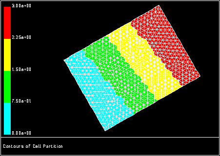
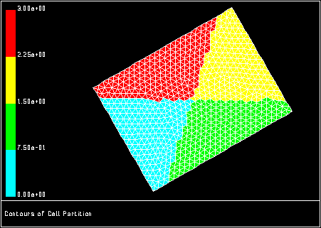
Stored Partition Count 2 To further aid interpretation of the partition information, you can draw contours of the mesh partitions (see the figures in Partition Methods).
![]() Results → Graphics → Contours
Results → Graphics → Contours ![]() Edit...
Edit...
To display the active cell partition or the stored cell partition (which were described above), select Active Cell Partition or Stored Cell Partition in the Cell Info... category of the Contours Of drop-down list, and turn off the display of Node Values (for details, see Displaying Contours and Profiles for information about displaying contours).
Important: If you have not already done so in the setup of your problem, you must perform a solution initialization in order to use the Contours dialog box.
If the speeds of the processors that will be used for a parallel
calculation differ significantly, you can specify a load distribution
for partitioning, using the load-distribution text command.
parallel → partition → set → load-distribution
For example, if you will be solving on three compute nodes, and one machine is twice as fast as the other two, then you may want to assign twice as many cells to the first machine as to the others (that is, a load vector of (2 1 1)). During subsequent mesh partitioning, partition 0 will end up with twice as many cells as partitions 1 and 2.
For this example, you need to start up Ansys Fluent such that compute node 0 is the fast machine, since partition 0, with twice as many cells as the others, will be mapped onto compute node 0. Alternatively, in this situation, you could enable the load balancing feature (described in Load Balancing) to have Ansys Fluent automatically attempt to discern any difference in load among the compute nodes.
When running a calculation using parallel Ansys Fluent, you may encounter a warning message in the console that reports problems related to the partitioning. The following is an example of such a warning:
#AMG# Warning: The global matrix size (1273286) is too large, and may
adversely affect the parallel performance. See the Ansys Fluent User's
Guide for information on troubleshooting partitioning issues.
The following are possible reasons for partitioning problems, along with recommendations for reducing them:
The presence of solid zones may cause a partition to have a very small amount of fluid cells, or none at all. To avoid this, it is recommended that you use the Metis method with automatic or manual partitioning; for the latter, you must ensure that Solid Zones weighting and model-weighted partitioning are enabled, with a suitable Value for the solid-to-fluid cell weighting (for example,
0.1).A partition may have a small number of cells if you have set up a load distribution for partitioning. Such settings should be disabled, by using the
load-distributiontext command (described in Load Distribution) and entering a value of1for each of the previously defined partitions.Some model settings (for example, shell conduction) can encapsulate some cells, which may cause difficulties with the coarsening process. To remedy this situation, you can either try a different partitioning method, or you can enable the global coarsening checking criteria with the following rpvar setting:
(rpsetvar 'amg/parallel/global-check-coarsening? #t)Coupled walls are encapsulated as part of the shell conduction model and S2S model. If you have partitioning problems, you can try reverting to the encapsulation routine used prior to version 16.0 by disabling the enhanced encapsulation:
define→models→shell-conduction→enhanced-encapsulation?