Ansys Fluent allows you to include heat transfer within the fluid and/or solid regions in your model. Problems ranging from thermal mixing within a fluid to conduction in composite solids can therefore be handled by Ansys Fluent.
When your Ansys Fluent model includes heat transfer you will need to enable the relevant physical models, supply thermal boundary conditions, and enter material properties (which may vary with temperature) that govern heat transfer. For information about heat transfer theory, see Heat Transfer Theory in the Theory Guide. Information about heat transfer theory and how to set up and use heat transfer in your Ansys Fluent model is presented in the following subsections:
The procedure for setting up a heat transfer problem is described below. Note that this procedure includes only those steps necessary for the heat transfer model itself; you will need to define the other settings (for example, other models, boundary conditions) as usual.
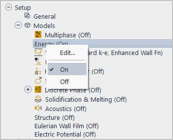
To activate the calculation of heat transfer, enable the energy equation by right-clicking Energy in the tree (under Setup/Models) and clicking On in the menu that opens.
 Setup →
Models → Energy
Setup →
Models → Energy
 On
On
(Optional, pressure-based solver only.) If you are modeling viscous flow and you want to include the viscous heating terms in the energy equation, enable the Viscous Heating option in the Viscous Model dialog box.
Setup →
Models → Viscous
Edit... As noted in Inclusion of the Viscous Dissipation Terms in the Theory Guide, the viscous heating terms in the energy equation are (by default) ignored by Ansys Fluent when the pressure-based solver is used. They are always included for the density-based solver. Viscous dissipation should be enabled when the shear stress in the fluid is large (for example, in lubrication problems) and/or in high-velocity, compressible flows. See Equation 5–10 in the Theory Guide.
Note: The Viscous Heating option should be enabled or disabled at the start of an unsteady simulation, and it is not recommended to change it during the calculation.
Define thermal boundary conditions at flow inlets, flow outlets, and walls. The boundary condition dialog boxes can be opened by right-clicking the boundary name in the tree (under Setup/Boundary Conditions) and clicking Edit... in the menu that opens; alternatively, you can open them from the Boundary Conditions task page:
Setup →  Boundary Conditions
At flow inlets and exits you will set the temperature; at walls you may use any of the following thermal conditions:
specified heat flux
specified temperature
convective heat transfer
external radiation
combined external radiation and external convective heat transfer
Thermal Boundary Conditions at Walls provides details on the model inputs that govern these thermal boundary conditions. The default thermal boundary condition at inlets is a specified temperature of 300 K; at walls the default condition is zero heat flux (adiabatic). See Cell Zone and Boundary Conditions for details about boundary condition inputs.
Important: If your heat transfer application involves two separated fluid regions, see the information provided below.
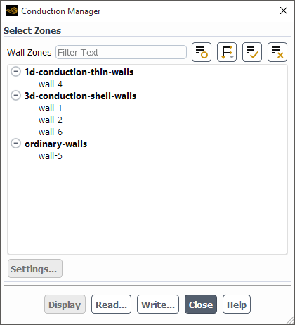
If your case involves conduction through walls (either 1d conduction through "thin" walls or 3d conduction through shell walls), you can specify the required settings for any wall using Figure 16.2: The Conduction Manager Dialog Box.
 Physics → Model
Specific → Conduction
Manager...
Physics → Model
Specific → Conduction
Manager...
Select any number of walls and click Settings....
Specify the conduction settings for the selected walls. For details, see Managing Conduction Walls.
Define material properties for heat transfer.
Setup →
Materials
Heat capacity and thermal conductivity must be defined, and you can specify many properties as functions of temperature as described in Physical Properties.
For stability reasons, Ansys Fluent includes a limit on the predicted temperature range. The purpose of the temperature ceiling and floor is to improve the stability of calculations in which the temperature should physically lie within known limits. Sometimes intermediate solutions of the equations give rise to temperatures beyond these limits for which property definitions, and so on, are not well defined.
The temperature limits keep the temperatures within the expected range for your problem. If the Ansys Fluent calculation predicts a temperature above the maximum limit, the stored temperature values are “pegged” at this maximum value. The default for the temperature ceiling is 5000 K. If the Ansys Fluent calculation predicts a temperature below the minimum limit, the stored temperature values are “pegged” at this minimum value. The default for the temperature minimum is 1 K.
If you expect the temperature in your domain to exceed 5000 K, use the Solution Limits dialog box to increase the Maximum Static Temperature.
![]() Solution →
Controls
Solution →
Controls
![]() Limits...
Limits...
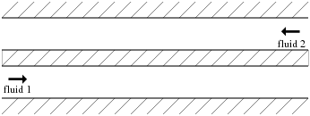
If your heat transfer application involves two fluid regions separated by a solid zone or a wall, as illustrated in Figure 16.3: Typical Counterflow Heat Exchanger Involving Heat Transfer Between Two Separated Fluid Streams, you will need to define the problem with some care. Specifically:
You should not use outflow boundary conditions in either fluid.
You can establish separate fluid properties by selecting a different fluid material for each zone. For species calculations, however, you can only select a single mixture material for the entire domain.
Figure 16.3: Typical Counterflow Heat Exchanger Involving Heat Transfer Between Two Separated Fluid Streams
Although many simple heat transfer problems can be successfully solved using the default solution parameters assumed by Ansys Fluent, you may accelerate the convergence of your problem and/or improve the stability of the solution process using some of the guidelines provided in this section.
When you use the pressure-based solver, Ansys Fluent under-relaxes the energy equation using the under-relaxation parameter defined by you in the Solution Controls task page, as described in Setting Under-Relaxation Factors.
![]() Solution →
Solution → ![]() Controls
Controls
If you are using the non-adiabatic non-premixed combustion model, you will set the energy under-relaxation factor as usual but you will also set an under-relaxation factor for temperature, as described below.
Ansys Fluent uses a default under-relaxation factor of 1.0 for the energy equation, regardless of the form in which it is solved (temperature or enthalpy). In problems where the energy field impacts the fluid flow (via temperature-dependent properties or buoyancy) you should use a lower value for the under-relaxation factor, in the range of 0.8–1.0. In problems where the flow field is decoupled from the temperature field (no temperature-dependent properties or buoyancy forces), you can usually retain the default value of 1.0.
When the enthalpy form of the energy equation is solved (that is, when you are using the non-adiabatic non-premixed combustion model), Ansys Fluent also under-relaxes the temperature, updating the temperature by only a fraction of the change that would result from the change in the (under-relaxed) enthalpy values. This second level of under-relaxation can be used to good advantage when you would like to let the enthalpy field change rapidly, but the temperature response (and its effect on fluid properties) to lag. Ansys Fluent uses a default setting of 1.0 for the under-relaxation on temperature and you can modify this setting using the Solution Controls task page.
![]() Solution →
Solution → ![]() Controls
Controls
If you are solving for species transport using the pressure-based solver and you encounter convergence difficulties, you may want to consider disabling the Diffusion Energy Source option in the Species Model dialog box.
![]() Setup → Models
→ Species
Setup → Models
→ Species
![]() Edit...
Edit...
When this option is disabled, Ansys Fluent will neglect the effects of species diffusion on the energy equation.
Note that species diffusion effects are always included when the density-based solver is used.
Often the most efficient strategy for predicting heat transfer is to compute an isothermal flow first and then add the calculation of the energy equation. The procedure differs slightly, depending on whether or not the flow and heat transfer are coupled.
If your flow and heat transfer are decoupled (no temperature-dependent properties or buoyancy forces), you can first solve the isothermal flow (energy equation turned off) to yield a converged flow-field solution and then solve the energy transport equation alone.
Important: Since the density-based solver always solves the flow and energy equations together, the procedure for solving for energy alone applies to the pressure-based solver, only.
You can temporarily disable the flow equations or the energy equation by deselecting them in the Equations dialog box:
![]() Solution →
Controls
Solution →
Controls
![]() Equations...
Equations...
You can also disable the energy equation:
![]() Setup →
Models → Energy
Setup →
Models → Energy
![]() Off
Off
If the flow and heat transfer are coupled (that is, your model includes temperature-dependent properties or buoyancy forces), you can first solve the flow equations before enabling energy. Once you have a converged flow-field solution, you can enable energy and solve the flow and energy equations simultaneously to complete the heat transfer simulation.
For conjugate heat transfer (CHT) problems, particularly those with combustion, the dominant time / iteration scales in the fluid and solid zones are often several orders of magnitude different. For transient simulations, solving the coupled fluid-solid interface with the same time step size for both fluid and solid domains is prohibitively expensive, and so Fluent allows for specifying a different time step size for solid domains. Such solid time stepping can be combined with a Loosely Coupled CHT options that provides instantaneous implicit and also time-averaged explicit options to couple fluid-solid interface, ensuring continuity of heat flow and temperature; this Loosely Coupled CHT option is also available for steady flows. You can also change the settings for solid zones that have an anisotropic thermal conductivity (other than biaxial).
Note:
For general CHT applications, the correct temporal evolution of temperature in the solid can only be obtained when the same time step size / number of iterations is used in fluid and solid zones.
For CHT simulations that have challenges in convergence and/or a discrepancy in the thermal predictions when running on parallel computing environments, it is recommended that you use BCGSTAB as a stabilization method (as mentioned in Setting the Stabilization Method), and ensure that the mesh is partitioned using Laplace smoothing (as mentioned in Preferences for Advanced Auto-Partitioning Methods).
For details, see the following sections:
When solving both the fluid and solid zones with a time step size that is suitable for the fluid zone, the computation of the energy equation at the solid zones becomes expensive. Specifying a larger time-step size accounts for the high thermal inertia of the solid zones which allows them to reach their thermal equilibrium faster. Note that the thermal field for the solid zones will still be updated at the same rate as fluid zones and they will remain fully coupled, so specifying a larger time step size by itself does not reduce redundant calculations or increase the performance.
You can enhance the performance of the simulation for some conjugate heat transfer cases by using the Loosely Coupled Conjugate Heat Transfer option along with the Specify Solid Time Step Size option. For details and limitations, see Loosely Coupled Conjugate Heat Transfer.
For a transient case with solid and fluid zones and the energy equation enabled, you can specify a different solid time step size using the Run Calculation task page:
![]() Solution → Run
Calculation
Solution → Run
Calculation
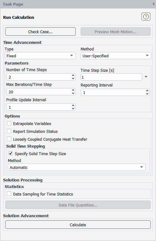
Under Options, enable the Specify Solid Time Step Size option.
Use the default Automatic time step size from the Method drop-down list to have the time step size calculated as described in Automatic Time Step Size Calculation; otherwise, select User-Specified to enter your own Time Step Size.
Note: You can enhance the performance of the simulation for some conjugate heat transfer cases by using the Loosely Coupled Conjugate Heat Transfer option along with the Specify Solid Time Step Size option. For details and limitations, see Loosely Coupled Conjugate Heat Transfer.
The default Automatic time step size is calculated by ANSYS Fluent using the following formula:
 | (16–1) |
where,
 is the representative length scale and is
calculated as
is the representative length scale and is
calculated as  .
. is
is  , the representative velocity scale, where
 is the conductivity,
  is the density, and
  is the specific heat capacity of the
solid.
is the specific heat capacity of the
solid.
The calculation for  results in an approximation for the solid time step
size, which might aide in the solution running more efficiently. It
should be noted, however, that this is only an engineering approximation
as there is no general way to calculate a meaningful length scale for an
arbitrary geometry.
results in an approximation for the solid time step
size, which might aide in the solution running more efficiently. It
should be noted, however, that this is only an engineering approximation
as there is no general way to calculate a meaningful length scale for an
arbitrary geometry.
For conjugate heat transfer (CHT) simulations, by default a fully coupled approach is used, so that the whole domain (including fluid and solid zones) is solved together and the energy field in the solids and fluids is solved and updated at every iteration / fluid time step. You can instead loosely couple the CHT, so that multi-domain architecture is used (within a single Fluent session) to compute the energy field in solid zones at only a few instants during the simulation, and thereby increase the speed of the simulation. With this approach, the temperature boundary condition from the solid zones is assigned to the fluid domain when the solid zones are not solved, and then periodically (at coupling) both the fluid and solid zones are solved based on your selection for Coupling Method.
Note: Loosely coupled CHT has following limitations and capabilities.
The case must have both fluid and solid zones.
The energy and flow equations must be enabled.
It is not available for the density-based solver.
It requires that the mesh does not change at the fluid-solid interface in order to be accurate. Therefore it is not supported when this interface undergoes remeshing and/or layering as part of a dynamic mesh or automatic adaption.
It is not available with porous zones.
It is not available if the case has a mesh interface that uses the Mapped option.
It is disabled if time-averaged explicit thermal coupling is already selected for one or more coupled walls. For details, see Time Averaged Explicit Thermal Coupling.
It is disabled if the case has shell conduction zones.
Time-averaged explicit thermal coupling (Time Averaged Explicit Thermal Coupling) and the Time-Averaged Explicit coupling method for Loosely Coupled CHT both employ the same explicit coupling method. The former solves the solid domain at each fluid time step, whereas the latter solves the solid domain at the specified coupling frequency.
You can loosely couple the CHT using the Run Calculation task page:
![]() Solution → Run
Calculation
Solution → Run
Calculation
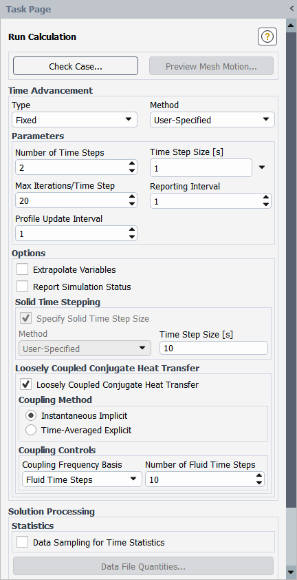
Under Options, enable the Loosely Coupled Conjugate Heat Transfer option.
For transient simulations, perform the following steps:
Make a selection from the Coupling Method list.
Instantaneous Implicit
This method solves the fluid-solid interface in a fully coupled manner like conventional coupled thermal boundary condition at each coupling step. For details, see Thermal Conditions for Two-Sided Walls.
Time-Averaged Explicit
In this method, Dirichlet – Neumann explicit thermal coupling is employed at each coupling step. A convective thermal boundary condition is applied at the wall adjacent to the solid and the instantaneous solid-side temperature is applied on the wall adjacent to the fluid. Time-averaged heat flow on the fluid side is used to compute the convective thermal boundary condition parameters (heat transfer coefficient and free-stream temperature) on the solid side.
Under Coupling Controls, make a selection from the Coupling Frequency Basis drop-down list:
Select Time to have the coupling performed at a set Time Period. This option is only available for the Instantaneous Implicit coupling method.
Select Fluid Time Steps to have the coupling performed at a set Number of Fluid Time Steps. This is not available when using adaptive time stepping.
If Time-Averaged Explicit is selected for the coupling method, Average Over (Time Steps) is shown for information only. This is the number of time steps used for computing time-averaged thermal variables. The input for this field is automatically copied from the specified Number of Fluid Time Steps.
The Specify Solid Time Step Size option is automatically enabled with the User-Specified method selected (note that the Automatic method is not available for transient simulations with loosely coupled CHT). You should ensure that the Time Step Size is equal to or larger than the period for the loose coupling.
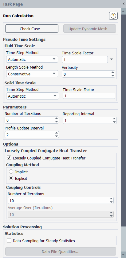
For steady simulations, perform the following steps:
Make a selection from the Coupling Method list.
Implicit
This method solves the fluid-solid interface in a fully coupled manner like conventional coupled thermal boundary condition at each iteration. For details, see Thermal Conditions for Two-Sided Walls.
Explicit
In this method, Dirichlet – Neumann explicit thermal coupling is employed at each coupling iteration. A convective thermal boundary condition is applied at the wall adjacent to the solid and the instantaneous solid-side temperature is applied on the wall adjacent to the fluid. Iteration-averaged heat flow on the fluid side is used to compute the convective thermal boundary condition parameters (heat transfer coefficient and free-stream temperature) on the solid side.
Under Coupling Controls, enter the Number of Iterations at which you want the coupling performed.
If Explicit is selected for coupling method, Average Over (Iterations) is shown for information only. This is the number of iterations used for computing iteration-averaged thermal variables. The input for this field is automatically copied from the specified Number of Iterations.
Note: The following practices are recommended:
For transient CHT simulations, it is recommended that you use a high coupling frequency at the beginning and gradually decrease the coupling frequency when the temperature of the solid zones starts to reach its equilibrium state. This will help in the rapid and smooth convergence of solid temperature without compromising of the performance gain.
Define the coupling frequency between fluid and solid to match the principal frequency of the fluid thermal field fluctuations, in order to improve accuracy.
For transient simulations involving conjugate heat transfer, you have the option of specifying a time averaged explicit coupling. This method solves the energy equation in the fluid and solid concurrently, which is different from the Loosely Coupled Conjugate Heat Transfer method, where solids are only solved with fluids when needed. The fluid and solid domains typically advance the solution at different time steps within each coupling cycle (see Specifying the Solid Time Step Size). Each coupling cycle is specified for a number of time steps at which the exchange of thermal boundary condition quantities occurs.
Well established Dirichlet – Neumann thermal coupling is employed at each cycle. At the end of each cycle, the convective thermal boundary condition is applied at the wall adjacent to the solid and the instantaneous solid side temperature is applied on the wall adjacent to the fluid. Time-averaged heat flow on the fluid side is used to compute the convective thermal boundary condition parameters (heat transfer coefficient and freestream temperature on the solid side).
You can enable this method for coupled walls from the Time Averaged Explicit Thermal Coupling dialog box:
![]() Physics →
Model Specific → Explicit Thermal
Coupling...
Physics →
Model Specific → Explicit Thermal
Coupling...
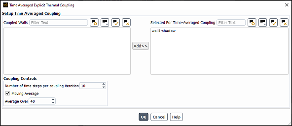
Select the wall pairs under Coupled Wall that you would like to convert to explicit time-averaged coupling.
Click Add>>. A prompt will appear warning that this operation slits the selected wall pairs (therefore altering the mesh). If you would like to retain the data for the current case, you should save the
.casand.datfiles before continuing.The walls selected for conversion will appear under Selected For Time-Averaged Coupling.
Under Coupling Controls, specify the Number of time steps per coupling iteration for the explicit coupling.
Optionally select Moving Average and specify Average Over. Fluent will still perform a coupling iteration with the frequency specified by Number of time steps per coupling iteration but will the use data averaged over the previous number of time steps as specified in Average Over.
In the above example shown in Figure 16.7: The Time Averaged Explicit Thermal Coupling Dialog Box, the first coupling iteration will occur at the 40th time step with averaged data over the first 40 time steps. The next coupling iteration will occur at the 50th time step using data averaged from the 10th to 49th time steps.
Upon enabling this option, Fluent automatically creates the required unsteady datasets for each coupled wall. For more information on unsteady statistics, see Inputs for Time-Dependent Problems.
Note the following limitations:
If you replace the mesh in your current case, you will have to redefine any transient explicit thermal coupled walls.
When performing a steady or transient conjugate heat transfer (CHT) simulation, you can change the following settings for pressure-based simulations that have the energy equation enabled and an anisotropic option (other than biaxial) selected for the thermal conductivity of the solid.
Heat Flux Methods
You can select the method used to calculate the heat flux for the anisotropic solid zones. The determining factor when choosing the method is whether the solid has highly anisotropic thermal conductivity properties (that is, has a conductivity in one direction that is more than 100 times the value in another direction), as such properties can result in convergence problems or reports that you are exceeding temperature limits. The following heat flux methods are available:
boundary-stabilized-implicitThis method is selected by default. It is robust for many cases with highly anisotropic solids, while only moderately increasing the number of iterations / time steps needed to reach convergence.
stabilized-implicitWhile this is the most robust method for cases with highly anisotropic solids, it also results in the greatest increase in the number of iterations / time steps needed to reach convergence of the available heat flux methods.
standardThis method results in the fastest convergence rate, but should only be used when the solid is not highly anisotropic.
To select the heat flux method for cases with anisotropic solids, use the following text command:
solve →
set → advanced
→ anisotropic-solid-heat-transfer
→ flux
Temperature Gradient Methods
You can select an improved method (named
local-neighbors) for calculating the temperature
gradient for the anisotropic solid zones. Compared to the default
standard method, the
local-neighbors method increases the speed of the
solid zone calculations to be 2–3 times faster.
To use the improved temperature gradient method, ensure that
Least Squares Cell Based is selected from the
Gradient drop-down list in the Solution
Methods task page, and then select the
local-neighbors method using the following text
command:
solve →
set → advanced
→ anisotropic-solid-heat-transfer
→ gradient
Relaxation for the Heat Flux Coefficient
You can reduce the relaxation for the heat flux coefficient to be less than the default value of 1 using the following text command. In certain anisotropic conductivity cases, such under-relaxation can help with convergence.
solve →
set → advanced
→ anisotropic-solid-heat-transfer
→ relaxation
For further details on anisotropic thermal conductivity properties, see Anisotropic Thermal Conductivity for Solids.
For information about postprocessing heat transfer quantities, see the following sections:
- 16.2.3.1. Available Variables for Postprocessing
- 16.2.3.2. Definition of Enthalpy and Energy in Reports and Displays
- 16.2.3.3. Reporting Heat Transfer Through Boundaries
- 16.2.3.4. Reporting Heat Transfer Through a Surface
- 16.2.3.5. Reporting Averaged Heat Transfer Coefficients
- 16.2.3.6. Exporting Heat Flux Data
Ansys Fluent provides reporting options for simulations involving heat transfer. You can generate graphical plots or reports of the variables listed under the Temperature... or Wall Fluxes... category. See Field Function Definitions for the list of available variables and their definitions.
The reported enthalpy values may be different between the pressure-based and density-based solver depending on the properties of the working fluid, compressible, incompressible, ideal gas, etc. For details, see the discussion of enthalpy in The Energy Equation in chapter 5, Heat Transfer of the Theory Guide.
You can use the Flux Reports dialog box to compute the heat transfer through each boundary of the domain, or to sum the heat transfer through all boundaries to check the heat balance.
![]() Results → Reports
→ Fluxes
Results → Reports
→ Fluxes
![]() Edit...
Edit...
It is recommended that you perform a heat balance check to ensure that your solution is truly converged.
Note:
For the Composition PDF Transport model, the Flux Reports dialog box reports the Total Heat Transfer Rate and Total Sensible Heat Transfer Rate only for the Lagrangian phase solution, which does not always guarantee overall mass conservation due to the nature of the discrete phase model. To check the balance of heat transfer rates that are based on the continuous phase computation, you should use the Surface Integrals dialog box to create a report for the Flow Rate of Enthalpy (Temperature category). (See Reporting Heat Transfer Through a Surface for details.)
Fluxes can only be computed on boundaries and not on interior or user defined surfaces such as planes, points, iso-surfaces, and so on.
You can use the Surface Integrals dialog box to compute the heat transfer through any boundary or any surface created using the methods described in Creating Surfaces and Cell Registers for Displaying and Reporting Data.
![]() Results → Reports
→ Surface Integrals
Results → Reports
→ Surface Integrals
![]() Edit...
Edit...
To report the mass flow rate of enthalpy
 | (16–2) |
choose Flow Rate for the Report Type in the Surface Integrals dialog box, select Enthalpy (in the Temperature... category) as the Field Variable, and select the surface(s) on which to integrate.
The Surface Integrals dialog box can also be used to
generate a report of averaged heat transfer coefficient  on a surface (
 ).
).
![]() Results → Reports
→ Surface Integrals
Results → Reports
→ Surface Integrals
![]() Edit...
Edit...
In the Surface Integrals dialog box, choose Area-Weighted Average for Report Type, select Surface Heat Transfer Coef. (in the Wall Fluxes... category) as the Field Variable, and select the surface.
It is possible to export heat flux data on wall zones (including radiation) to
a generic file that you can examine or use in an external program. To save a
heat flux file, you will use the custom-heat-flux text
command.
file → export
→ custom-heat-flux
Heat transfer data will be exported in the following free format for each face zone that you select for export:
 zone-name nfaces
 x_f y_f z_f A Q T_w T_c HTC
 .
 .
 .
Each block of data starts with the name of the face zone
(zone-name) and the number of faces in the zone
(nfaces). Next there is a line for each face (that
is, nfaces lines), each containing the components of
the face centroid (x_f, y_f,
and, in 3D, z_f), the face area
(A), the heat transfer rate
(Q), the face temperature
(T_w), the adjacent cell temperature
(T_c), and the heat transfer coefficient
(HTC). If the heat transfer coefficient is
calculated based on wall function (Equation 42–69),
then  is the convective heat transfer rate. Otherwise,
 will be the total heat transfer rate, including radiation heat
transfer.
will be the total heat transfer rate, including radiation heat
transfer.
For information on how to include the effects of natural convection in buoyancy-driven flow problems, see Buoyancy-Driven Flows and Natural Convection.
For information about shell conduction considerations, see the following sections:
By default, Ansys Fluent treats walls as having zero-thickness and presenting no thermal resistance to heat transfer across them. If a thickness is specified for a wall (thereby making it a thin wall, as described in Thin-Wall Thermal Resistance Parameters) then the appropriate thermal resistance across the wall thickness is imposed, although conduction is considered in the wall in the normal direction only. There are applications, however, where conduction in the planar directions of the wall is also important. For these applications, you have two options: you can either mesh the thickness, or you can use the shell conduction approach. Shell conduction can be used to model one or more layers of wall cells without the need to mesh the wall thickness in a preprocessor. When the shell conduction approach is utilized, you have the ability to easily switch on and off conjugate heat transfer on any wall. If you create a shell—either by enabling Shell Conduction in an individual Wall dialog box (as described in Shell Conduction) or by defining multiple walls as shell conduction zones using the Conduction Manager dialog box (as described in Managing Conduction Walls)—and define the settings for the shell layer(s) using the Conduction Layers dialog box, then Ansys Fluent will automatically grow the specified layers of cells. The cells that are grown will be either prism cells or hex cells, depending on the type of face mesh that is utilized; at no point are the cells visible in the displayed mesh.
Shell conduction can be used to account for thermal mass in transient thermal analysis problems (see Locking the Temperature for Solid and Shell Zones for more information). It can also be used for multiple junctions and allows heat conduction through the junctions. Shell conduction can be applied on boundary walls as well as two-sided walls.
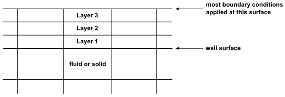
In the case where shell conduction is applied on a boundary wall, the original surface is referred to as the “wall surface” and is always adjacent to the fluid / solid cells. The first time the shell model is enabled at any wall surface, Fluent grows the required shell zones. These layers are numbered sequentially, starting with the one closest to the wall surface. See Figure 16.8: A Boundary Wall with Shell Conduction for a visualization of how the solver treats shells.
For the most part, the boundary conditions that you specify for the boundary wall are applied to the layer surface that is furthest from the wall surface; only the internal emissivity is applied at the wall surface. The sides of the shell zone require boundary conditions as well. If the shell is connected to another wall that does not have shell conduction enabled, the shell side will take the boundary condition of the attached wall. The sides will be adiabatic if they are connected to face zones that have a boundary condition type other than wall. If the attached wall has shell conduction enabled, then the common sides at the junction will be coupled.
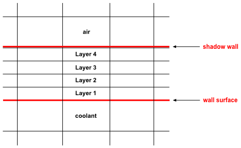
The layers of cells grown for two-sided walls can be visualized in a similar way to Figure 16.8: A Boundary Wall with Shell Conduction, except that the layer surface that is furthest from the wall surface is also adjacent to a shadow wall (which is then adjacent to the other fluid / solid zone).
The following is a list of limitations for the shell conduction model:
Shell conduction only supports constant wall thickness.
Shell conduction cannot be used on moving wall zones.
Shell conduction cannot be used with FMG initialization.
Shell conduction is not available when the wall is set up to receive thermal data via system coupling.
Shell conduction is not available for 2D.
Shell conduction is available only when the pressure-based solver is used.
Shell conducting walls cannot be split or merged. If you need to split or merge a shell conducting wall, you will need to turn off the Shell Conduction option for the wall (in the Wall dialog box), perform the split or merge operation, and then enable Shell Conduction for the new wall zones.
The shell conduction model cannot be used on a wall zone that has undergone hanging node adaption. If you want to perform such adaption elsewhere in the computational domain, be sure to use a boolean operation in an adaption expression to exclude a register containing the shell conducting walls. For example,
NOT(region_0). Refer to Adapting the Mesh for additional information on adapting the mesh.Fluxes at the ends of a shell conducting wall are not included in heat balance reports. These fluxes are accounted for correctly in the Ansys Fluent solution, but are not listed in the flux report.
For a one-sided wall with shell conduction model enabled, the specified thermal BC is applied to the external surface (side of the wall away from the domain). Therefore, the reported flux on the wall would not correspond to the specified thermal BC.
The junction of a wall with shell conduction enabled and a non-conformal coupled wall is not supported. Such a junction will not be thermally connected, that is, there will be no heat transfer between the shell and the mesh interface wall.
When running the parallel solver with the shell conduction model, note that coupled walls are encapsulated. If you encounter problems with the partitioning of the mesh, you can try changing the encapsulation method to see if that resolves the problem (see Troubleshooting for this and other troubleshooting options).
Shells with a sharp bend may yield non-physical temperature fields when using Green-Gauss Node Based gradients. This applies to any angle (acute or obtuse) with the effect worsening as the angle approaches 90 degrees. To resolve the issue, you should consider breaking the sharp angled shells into multiple shells or, in the event that this cannot be done, enabling Warped Face Gradient Correction.
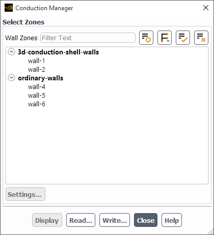
The Conduction Manager dialog box provides a convenient way for you to manage, define, and display multiple conduction zones. You can
display any wall zone
enable or disable shell conduction for a wall
define the settings for conduction walls or shell layers, such as thickness, material, and heat generation rate
Note that you can still enable shell conduction for a wall and define the related settings using the Wall dialog box, as described in Shell Conduction. However, the Conduction Manager dialog box provides you with an alternative to do such activities from a single dialog box for all the walls, instead of visiting the individual Wall boundary condition dialog boxes.
![]() Physics → Model
Specific → Conduction Manager...
Physics → Model
Specific → Conduction Manager...
To manage shell conduction using the Conduction Manager dialog box, perform the following steps:
(optional) If you have previously generated a CSV file that contains shell conduction settings for the layers of the walls, you can read it by clicking at the bottom of the Conduction Manager dialog box and using the dialog box that opens; otherwise, you should proceed to the steps that follow.
Using a
.csvfile can be helpful when you have a large number of layers and walls. It is not necessary to create the.csvfile from nothing, as you can create a simplified.csvfile with sample values using the button, and then revise the settings using a spreadsheet program. See Conduction Settings File Format for details about the format of the.csvfile.Select the walls you want to convert to shell conduction and click Settings.... The Conduction Layer dialog box opens.
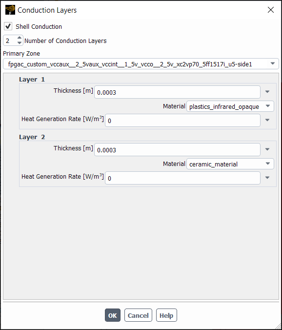
Select Shell Conduction to enable shell conduction for the selected walls.
Note: If the Shell Conduction option is disabled and you specify a thickness, the wall(s) will be treated as thin walls (1d conduction).
If you have selected multiple walls, you can assign one to be the Primary Zone. The settings for the Primary Zone will be copied to the other walls that are currently selected.
Specify the number of layers, and then define the thickness, material, and heat generation rate for each layer. Note that you have the option of defining the heat generation rate using a user-defined function (UDF) that utilizes the
DEFINE_PROFILEmacro; for more information on creating and using user-defined functions, see the Fluent Customization Manual.Important: You must specify a nonzero-thickness for every layer.
Click to save your settings for the selected walls and close the Conduction Layers dialog box.
The walls that have shell conduction enabled will appear listed under 3d-conduction-shell-walls on Figure 16.10: The Conduction Manager Dialog Box.
If you want to save all of the settings you specified using the Conduction Manager dialog box as a
.csvfile, click and specify a name in the dialog box that opens. You can edit the conduction settings in this.csvfile using a spreadsheet program, and then read it in this or a separate case file, as described in step 1. Note that information will not be written for any wall that defines the heat generation rate using a UDF.
Note that you have the option of disabling shell conduction in every wall with a single action, by using the following text command. This capability is available in both serial and parallel mode.
define →
boundary-conditions →
modify-zones →
delete-all-shells
Shell zones can be patched using the Patch dialog box, as described in Patching Values in Selected Cells.
![]() Solution →
Initialization
Solution →
Initialization
![]() Patch...
Patch...
You can lock (or “freeze”) the temperature values for all the
cells in shells and solid zones (including those to which you have a hooked an
energy source through a UDF) by using the
solve/set/lock-solid-temperature? text command, as
described in Locking the Temperature for Solid and Shell Zones.
In order to facilitate the postprocessing of shells, surfaces (referred to as “shell surfaces”) are created at the interface of adjacent layers, as well as at the layer surface that is furthest from the wall surface. Note that shell surfaces are not created on the sides of the shell zones or in the interior of the layers. The shell surfaces can then be selected from the Surfaces list available in a variety of dialog boxes (for example, the Contours dialog box, the Surface Report Definition dialog box, and the Solution XY Plot dialog box) in the same way as the surfaces for the wall and (for two-sided walls) the shadow wall. When visualized in the graphics display window, these shell surfaces will be coincident with the wall they are associated with.
The default naming convention for these shell surfaces is <wall_name>-<c0>:<c1>, where:
<wall_name> is the name of the wall on which the layers have been grown.
<c0> is the rank of the layer on the c0 side of the interface (that is, the layer closest to the wall surface).
<c1> is the rank of the layer on the c1 side of the interface (that is, the layer furthest from the wall surface). Note that the layer surface that is furthest from the wall surface does not have a layer on the c1 side, and so a different convention is used: for boundary walls, <c1> is set to external; for two-sided walls, <c1> is set to the name of the fluid / solid adjacent to the shadow wall.
You have the ability to rename the shell surfaces, if you want. The following figures illustrate the default naming convention, where the wall/shadow surfaces are displayed in red and the shell surfaces are displayed in black.
You can use the walls, shadow walls, and shell surfaces to display the temperature of the interfaces and adjacent cells. The Temperature... category provides two options: the temperature of the cell on the c0 side of the surface is stored as Static Temperature; and the temperature of the surface itself is stored as Wall Temperature. If a more detailed analysis of the solid zone and surfaces is required, then you should consider creating layers of solid cells in your meshing application.
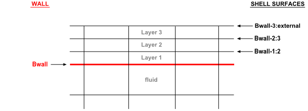
The following examples illustrate how to postprocess the surfaces shown in Figure 16.12: Shell Surface Names for a Boundary Wall:
The contours of Static Temperature and Wall Temperature of Bwall will provide the temperature of the fluid cells adjacent to Bwall and the temperature of the Bwall surface itself, respectively.
The contours of Static Temperature and Wall Temperature of Bwall-1:2 will provide the temperature of the cells of Layer 1 and the temperature of the interface between Layer 1 and Layer 2 (that is, the Bwall-1:2 shell surface), respectively.
The contours of Static Temperature and Wall Temperature of Bwall-3:external will provide the temperature of the cells of Layer 3 and the temperature of the layer surface that is furthest from the wall surface (that is, the Bwall-3:external shell surface), respectively.
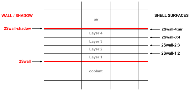
The following examples illustrate how to postprocess the surfaces shown in Figure 16.13: Shell Surface Names for a Two-Sided Wall:
The contours of Static Temperature and Wall Temperature of 2Swall-4:air will provide the temperature of the cells of Layer 4 and the temperature of the interface between Layer 4 and the shadow wall (that is, the 2Swall-4:air shell surface), respectively.
The contours of Static Temperature and Wall Temperature of 2Swall-shadow will provide the temperature of the air cells adjacent to 2Swall-shadow and the temperature of the shadow wall, respectively.
When postprocessing shells, note the following limitations/considerations:
You should not enable Node Values when postprocessing any surfaces associated with shells surfaces. The layers share nodes at the edges, and thus the averaging at such nodes is erroneous.
You cannot postprocess shells in Ansys CFD-Post, as shell surfaces are not supported.
The Boundary Values option can be used for displaying contours on shell surfaces. The values with this option for Wall Temperature and Static Temperature are identical for shell surfaces.
When post-processing the following options on shell surfaces, like any other surface, boundary values are considered:
Surface report definitions
XY Plot
Thermal conductivity can be defined using direction vectors but these directions are constant and therefore only relevant for geometries that are aligned with the global coordinate system. This feature allows the definition of anisotropic thermal conductivity where the anisotropy follows the shape of the geometry. This can be useful in defining anisotropic thermal conductivity for twisted geometries such as electric motor coils/windings.
To provide flexibility in handling such scenarios, a Curvilinear Coordinate System (CCS) that follows the shape of the geometry can be defined.
For more details on anisotropic conductivity, see Anisotropic Conductivity in Solids in the Fluent Theory Guide.
The general workflow for setting up anisotropic thermal conductivity is as follows:
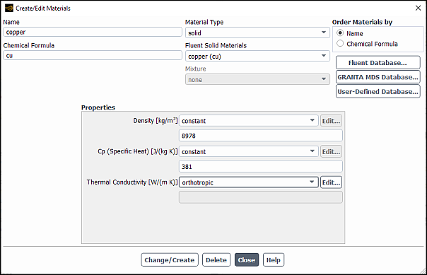
For the solid material, set the Thermal Conductivity to orthotropic.
Physics
→ Materials
→ Create/Edit...
Define a Curvilinear Coordinate System that follows the shape of the geometry. For details, see Curvilinear Coordinate Systems.
Setup →
Curvilinear Coordinate
System New...
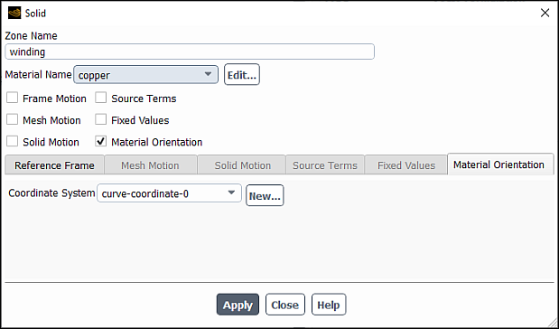
Assign the CCS to the appropriate cell zone.
Setup →
Cell Zone
Conditions → Solid → <cell
zone name> Edit...
Select Material Orientation.
On the Material Orientation sub-panel, for Coordinate System, select the CCS you created in step 2.
If for Coordinate System you specify the default From Material, Fluent uses the directions specified in the Orthotropic Conductivity dialog box.