


During the solution process you can monitor the convergence dynamically by checking residuals, statistics, force values, surface integrals, and volume integrals. You can print reports of or display plots of lift, drag, and moment coefficients, surface integrations, and residuals for the solution variables. For unsteady flows, you can also monitor elapsed time. Creating report definitions for monitoring is described in Creating Report Definitions. See Embedded Graphics Window Dashboards for additional techniques that can be used to monitor the solution as it evolves.
For additional information, see the following sections:
At the end of each solver iteration, the residual sum for each of the conserved variables is computed and stored, thereby recording the convergence history. This history is also saved in the data file. The residual sum is defined below.
On a computer with infinite precision, these residuals will go to zero as the solution converges. On an actual computer, the residuals decay to some small value (“round-off”) and then stop changing (“level out”). For single-precision computations (the default for workstations and most computers), residuals can drop as many as six orders of magnitude before hitting round-off. Double-precision residuals can drop up to twelve orders of magnitude. Guidelines for judging convergence can be found in Judging Convergence.
After discretization, the conservation equation for a general variable  at a cell
  can be written as
 | (36–25) |
Here  is the center coefficient,
  are the influence coefficients for the neighboring cells, and
  is the contribution of the constant part of the source term
  in
in  and of the boundary conditions. In Equation 36–25,
 | (36–26) |
The residual  computed by Ansys Fluent's pressure-based solver is the imbalance in Equation 36–25 summed
over all the computational cells
computed by Ansys Fluent's pressure-based solver is the imbalance in Equation 36–25 summed
over all the computational cells  . This is referred to as the unscaled residual. It may be written as
 | (36–27) |
In general, it is difficult to judge convergence by examining the residuals defined by Equation 36–27
since no scaling is employed. This is especially true in enclosed flows such as natural convection in a room where there is no
inlet flow rate of  with which to compare the residual.
Ansys Fluent scales the residual using two kinds of scaling factors, representative of the flow rate of  through the domain. The factors are termed global scaling and local
scaling. The type of scaling can be selected from the Residual Monitors dialog box. The
“globally scaled” residual is defined as
through the domain. The factors are termed global scaling and local
scaling. The type of scaling can be selected from the Residual Monitors dialog box. The
“globally scaled” residual is defined as
 | (36–28) |
There are two instances where  is modified in the denominator term
  : for momentum equations, it is replaced with the magnitude of
the velocity at cell
: for momentum equations, it is replaced with the magnitude of
the velocity at cell  ; and for Reynolds stress equations, it is replaced with the
trace of the Reynolds stress tensor at cell divided by the number of dimensions of the case (2D or
3D).
; and for Reynolds stress equations, it is replaced with the
trace of the Reynolds stress tensor at cell divided by the number of dimensions of the case (2D or
3D).
The “locally scaled” residual is defined as
 | (36–29) |
Note that for the momentum and Reynolds stress equations,  and
and  are modified in the same manner as for global scaling.
The scaled residual is a more appropriate indicator of convergence for most problems. The selection of scaling and convergence criteria for different types of scaling are discussed in Judging Convergence. The default residuals displayed by Ansys Fluent are global scaling.
For the continuity equation, the unscaled residual for the pressure-based solver is defined as
 | (36–30) |
The local scaling is the same for all equations, except for the continuity residual, which by default uses the following enhanced formulation:
 | (36–31) |
where  is the unscaled continuity residual defined in Equation 36–30 for a cell
  ,
,  is the mass flow rate at face
  of the cell,
  is the total number of faces for the cell, and
  is the total number of cells in the domain. This enhanced formulation is recommended, as the use of the absolute
mass flow rate at each cell can produce behavior that is more consistent with the other residuals. Note that after you have
enabled the Compute Local Scale option in the Residual Monitors dialog box (as described
in a later section), you have the option of disabling this enhanced formulation for the continuity residual by using the following
text command, so that it is instead calculated according to Equation 36–29 like the other residuals:
is the total number of cells in the domain. This enhanced formulation is recommended, as the use of the absolute
mass flow rate at each cell can produce behavior that is more consistent with the other residuals. Note that after you have
enabled the Compute Local Scale option in the Residual Monitors dialog box (as described
in a later section), you have the option of disabling this enhanced formulation for the continuity residual by using the following
text command, so that it is instead calculated according to Equation 36–29 like the other residuals:
solve/monitors/residual/enhanced-continuity-residual?.
The global scaling also treats continuity in a unique way, and it is defined as
 | (36–32) |
The denominator is the largest absolute value of the continuity residual in the first five iterations.
The scaled residuals described above are useful indicators of solution convergence. Guidelines for their use are given in Judging Convergence. It is sometimes useful to determine how much a residual has decreased during
calculations as an additional measure of convergence. For this purpose, Ansys Fluent allows you to normalize the residual (either
scaled or unscaled) by dividing by the maximum residual value after  iterations, where
  is set by you in the Residual Monitors Dialog Box in the Iterations field
under Residual Values.
is set by you in the Residual Monitors Dialog Box in the Iterations field
under Residual Values.
 | (36–33) |
Normalization in this manner ensures that the initial residuals for all equations are of  and is sometimes useful in judging overall convergence.
By default,  . You can also specify the normalization factor (the denominator in Equation 36–33)
manually in the Residual Monitors Dialog Box.
. You can also specify the normalization factor (the denominator in Equation 36–33)
manually in the Residual Monitors Dialog Box.
A residual for the density-based solver is simply the time rate of change of the conserved variable ( ). The RMS residual is the square root of the average of the squares of the residuals in each cell of the
domain:
). The RMS residual is the square root of the average of the squares of the residuals in each cell of the
domain:
 | (36–34) |
Equation 36–34 is the unscaled residual sum reported for all the coupled equations solved by Ansys Fluent’s density-based solver.
Important: The residuals for the equations that are solved sequentially by the density-based solver (turbulence and other scalars, as discussed in Density-Based Solver in the Theory Guide) are the same as those described above for the pressure-based solver.
In general, it is difficult to judge convergence by examining the residuals defined by Equation 36–34 since no scaling is employed. This is especially true in enclosed flows such as natural convection in a room where there is no
inlet flow rate of  with which to compare the residual. As with the pressure-based solver, Ansys Fluent uses two types of scaling for
the density-based solver. The globally scaled residual is defined as
with which to compare the residual. As with the pressure-based solver, Ansys Fluent uses two types of scaling for
the density-based solver. The globally scaled residual is defined as
 | (36–35) |
The denominator is the largest absolute value of the residual in the first five iterations.
The locally scaled residual is calculated from the local flux imbalance in the cell. It is calculated using Equation 36–36 :
 | (36–36) |
 is the conservative variable and
  is the cell volume. The unscaled residual is always calculated from Equation 36–34.
The scaled residuals described above are useful indicators of solution convergence. Guidelines for their use are given in Judging Convergence. It is sometimes useful to determine how much a residual has decreased during
calculations as an additional measure of convergence. For this purpose, Ansys Fluent allows you to normalize the residual (either
scaled or unscaled) by dividing by the maximum residual value after  iterations, where
  is set by you in the Residual Monitors Dialog Box in the Iterations field
under Residual Values.
is set by you in the Residual Monitors Dialog Box in the Iterations field
under Residual Values.
Normalization of the residual sum is accomplished by dividing by the maximum residual value after  iterations, where
  is set by you in the Residual Monitors Dialog Box in the Iterations field
under Residual Values :
is set by you in the Residual Monitors Dialog Box in the Iterations field
under Residual Values :
 | (36–37) |
Normalization in this manner ensures that the initial residuals for all equations are of  and is sometimes useful in judging overall convergence.
By default,  , making the normalized residual equivalent to the scaled
residual. You can also specify the normalization factor (the denominator in
Equation 36–37) manually in the Residual Monitors Dialog Box.
, making the normalized residual equivalent to the scaled
residual. You can also specify the normalization factor (the denominator in
Equation 36–37) manually in the Residual Monitors Dialog Box.
All inputs controlling the monitoring of residuals are entered using the Residual Monitors Dialog Box (Figure 36.36: The Residual Monitors Dialog Box).
![]() Solution → Reports → Residuals...
Solution → Reports → Residuals...
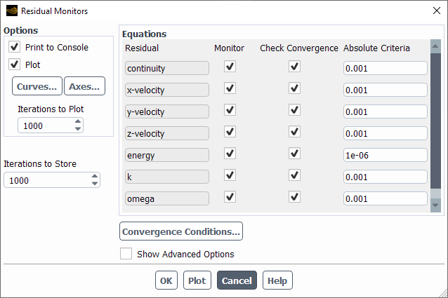
In general, you will only need to enable residual plotting and modify the convergence criteria using this dialog box. Additional controls are available for disabling monitoring of particular residuals, and modifying normalization and plot parameters.
By default, residual values for all relevant variables are printed in the console after each iteration. If you want to disable this printout, turn off Print to Console under Options. To enable the plotting of residuals after each iteration, turn on Plot under Options. Residuals will be plotted in the graphics window during the calculation.
If you want to display a plot of the current residual history, simply click the push button.
Residual histories for each variable are automatically saved in the data file, regardless of whether they are being monitored. You can control the number of history points to be stored by changing the Iterations to Store entry. By default, up to 1000 points will be stored. If more than 1000 iterations are performed (that is, the limit is reached), every other point will be discarded—leaving 500 history points—and the next 500 points will be stored. When the total hits 1000 again, every other point will again be discarded, and so on. If you are performing a large number of iterations, you will lose a great deal of residual history information at the beginning of the calculation. In such cases, you should increase the Iterations to Store value to a more appropriate value. Of course, the larger this number is, the more memory you will need, the longer the plotting will take, and the more disk space you will need to store the data file.
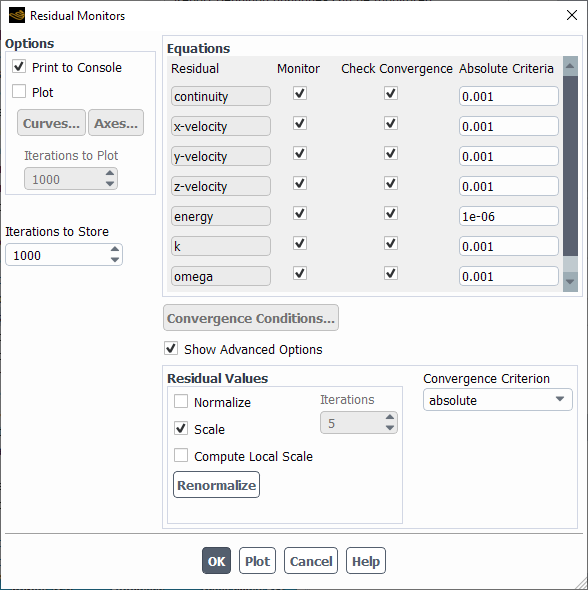
Options for controlling normalization and scaling are found by enabling Show Advanced Options in the Residual Monitors dialog box (Figure 36.37: The Residual Monitors Dialog Box with Advanced Options Shown).
By default, scaling of residuals (see Equation 36–28, Equation 36–32, or Equation 36–35) is enabled and the default convergence criterion is 10-6 for energy, DO, and P-1 equations and 10-3 for all other equations. When the Scale option is enabled, global scaling will be applied by default. You can then enable the Compute Local Scale option and select the Reporting Option from the drop-down list. You have a choice to plot or print to the console the local scaling or the global scaling of residuals. By default, the global scaling of residuals will be plotted. If local scaling is selected, the default convergence criterion for every equation is changed to 10-5 for steady cases or 10-4 for transient cases.
Note:
When Compute Local Scale is enabled, Ansys Fluent computes and stores both the locally and globally scaled residuals from subsequent iterations, for the purpose of reporting. The scaled residuals are stored in the data file.
You can enable Local Residual Scaling in Preferences (Simulation branch) to have local residuals plotted by default.
Important: Once the Compute Local Scale option is enabled and you disable the Scale option, the Compute Local Scale option will not automatically be disabled. Instead, it will compute both the locally and globally scaled residuals, but only print or plot the unscaled residual.
Residual normalization (that is, dividing the residuals by the largest value during the first few iterations) is also available but disabled by default.
Normalization can be used with both scaled and unscaled residuals. Note that if normalization is enabled, the convergence criterion may need to be adjusted appropriately. See Judging Convergence for information about judging convergence based on the different types of residual reports. (Both the raw residuals and scaling factors are stored in the data file, so you can switch between scaled and unscaled residuals.)
To report unscaled residuals, simply disable the Scale option under Residual Values.
Important: If you switch from scaled to unscaled residuals (or vice versa) and you are normalizing the residuals (as described below), you must click the button to recompute the normalization factors.
If you want to normalize the residuals (see Equation 36–33 or Equation 36–37), enable the Normalize option under Residual
Values. The Normalization Factor column will be
added to the dialog box at this time. Ansys Fluent will normalize the printed
or plotted residual for each variable by the value indicated as the
Normalization Factor for that variable. The default
Normalization Factor is the maximum residual value after
the first 5 iterations. To use the maximum residual value after a different
number of iterations (that is, specify a different value for  in Equation 36–33 or Equation 36–37), you can modify the
Iterations entry under Residual
Values.
in Equation 36–33 or Equation 36–37), you can modify the
Iterations entry under Residual
Values.
In some cases, the maximum residual may occur sometime after the iteration specified in the Iterations field. If this should occur, you can click the button to set the normalization factors for all variables to the maximum values in the residual histories. Subsequent plots and printed reports will use the new normalization factor.
You can also specify the normalization factor (the denominator in Equation 36–33 or Equation 36–37) explicitly. To modify the normalization factor for a particular variable, enter a new value in the corresponding Normalization Factor field in the Residual Monitors Dialog Box.
If you want to report unnormalized, unscaled residuals (Equation 36–27 or Equation 36–34), disable the Normalize and Scale options under Residual Values in the Residual Monitors Dialog Box. Note that unnormalized, unscaled residuals are stored in the data file regardless of whether the reported residuals are normalized or scaled.
With Show Advanced Options enabled, you have the ability to choose certain convergence criteria, which provides you with alternative ways to check convergence when using the iterative transient solver. The various convergence criteria can be selected in the Residual Monitors dialog box from the Convergence Criterion drop-down list (Figure 36.38: The Residual Monitors Dialog Box Displaying Relative or Absolute Convergence).
![]() Solution → Reports → Residuals...
Solution → Reports → Residuals...
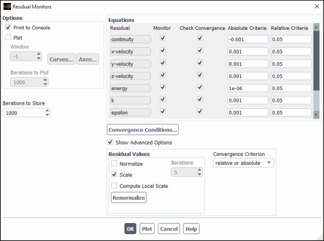
Four options are available for checking an equation for convergence:
- absolute
This is the default. For steady-state cases, absolute and none are the only options available for selection. The residual (scaled and/or normalized) of an equation at an iteration is compared with a user-specified value. If the residual is less than the user-specified value, that equation is deemed to have converged for a time step.
- relative
The residual of an equation at an iteration of a time step is compared with the residual at the start of the time step. If the ratio of the two residuals is less than a user-specified value, that equation is deemed to have converged for a time step.
- relative or absolute
If either the absolute convergence criterion or the relative convergence criterion is met, the equation is considered converged.
The Relative Criteria can be set when relative or relative or absolute is selected.
- none
Convergence checking is disabled.
In many situations, the absolute convergence criterion could be too stringent for transient flows causing a large number of iterations per time step. For example, the scaling of the continuity equation is based on the value of the continuity residual in the first five iterations. The scaling factor could be low if the initial continuity residual is small and therefore the scaled residual could fail to meet the absolute convergence criterion. With the relative convergence criterion, convergence is checked by comparing the residual at an iteration of a time step with the residual at the beginning of the time step and hence this problem is alleviated. The relative or absolute convergence criterion is useful in situations where the residuals of some of the equations are already very low at the start of a time step (for example, when a particular variable has reached steady-state), and the order of magnitude reduction in residuals is not possible. The none option allows you to disable convergence checking by selecting the option in the Convergence Criterion drop-down list.
Important: relative and relative or absolute convergence criteria are available only with the unsteady pressure-based solver and unsteady density-based solver.
The text command used to access the convergence criterion is
solve → monitors → residual
→ criterion-type
When criterion-type is entered, you will have the following choices:
| Criterion | Type |
|---|---|
| 0 | absolute |
| 1 | relative |
| 2 | relative or absolute |
| 3 | none |
For criterion-type 1 or 2, the text command
relative-conv-criteria will appear under the residual text menu, where the
various relative-conv-criteria can be set.
Important: If the NITA solver is enabled, no convergence criteria are available for selection.
Depending on the Convergence Criterion you choose, Ansys Fluent will check for convergence. If convergence is being monitored, the solution will stop automatically when each variable meets its specified convergence criterion. Convergence checks can only be performed on variables whose residuals are being monitored (variables with the Monitor option enabled).
You can choose whether or not you want to check the convergence for each variable by enabling or disabling the Check Convergence option for it in the Residual Monitors Dialog Box. To modify the convergence criterion for a particular variable, enter a new value in the corresponding convergence criterion field.
If your problem requires the solution of many equations (for example, turbulence quantities and multiple species), a plot that includes all residuals may be difficult to read. In such cases, you may choose to monitor only a subset of the residuals, perhaps those that affect convergence the most. You can indicate whether or not you want to monitor residuals for each variable by enabling or disabling the relevant check box in the Monitor list of the Residual Monitors Dialog Box.
If you choose to plot the residual values (either interactively during the solution or using the Plot button after calculations are complete), there are several display parameters you can modify.
In the Window field under Options, you can specify the ID of the graphics window in which the plot will be drawn. When Ansys Fluent is iterating, the active graphics window is temporarily set to this window to update the residual plot, and then returned to its previous value. Thus, the residual plot can be maintained in a separate window that does not interfere with other graphical postprocessing.
You can modify the number of residual history points to be displayed in the plot by changing the Iterations to
Plot entry under Options. If you specify  points, Ansys Fluent will display the last
  history points. Since the
  axis is scaled by the minimum and maximum values of all points in the plot, you can zoom in on the end of the
residual history by setting Iterations to Plot to a value smaller than the number of iterations performed.
If, for example, the residuals jumped early in the calculation when you turned on turbulence, that peak broadens the overall range
in residual values, making the smaller fluctuations later on almost indistinguishable. By setting the value of
Iterations to Plot so that the plot does not include that early peak, your
axis is scaled by the minimum and maximum values of all points in the plot, you can zoom in on the end of the
residual history by setting Iterations to Plot to a value smaller than the number of iterations performed.
If, for example, the residuals jumped early in the calculation when you turned on turbulence, that peak broadens the overall range
in residual values, making the smaller fluctuations later on almost indistinguishable. By setting the value of
Iterations to Plot so that the plot does not include that early peak, your  -axis range is better suited to the values that you are interested in seeing. For more information on residual
history points, refer to the discussion of storing residual history points, described earlier in this section.
-axis range is better suited to the values that you are interested in seeing. For more information on residual
history points, refer to the discussion of storing residual history points, described earlier in this section.
You can also modify the attributes of the plot axes and the residual curves. Click the or Curves... button to open the Axes Dialog Box or Curves Dialog Box. See Axes Dialog Box and Curves Dialog Box for details.
Important: Note that entering a value for Iterations to Plot does not necessarily mean solved iterations but rather stored (or sampled) data points. Note also that the frequency of the data storage will diminish towards the start of the solution as the number of solved iterations increases. Due to this, whenever the stored iterations is greater than the solved iterations, if you plot n iterations, you actually see a history that goes back further than n solved iterations.
If you are having solution convergence difficulties, it is often useful to plot the residual value fields (for example, using contour plots) to determine where the high residual values are located. By default, only the time step (for the density-based solver) and the mass imbalance (for the pressure-based solver) in each cell is available.
If you want to plot residual value fields for additional residual value fields, you will need to do the following:
Read in the case and data files of interest (if they are not already in the current session).
Use the following text command to enable the saving of residual values.
solve→set→advanced→retain-cell-residualsPerform at least one iteration.
The solution variables for which residual values are available will appear in the Residuals... category in the postprocessing dialog boxes. Note that residual values are not available for the radiative transport equations solved by the discrete ordinates radiation model.
Important: The residual values that are made available for postprocessing are the unscaled values.
If you are solving a fully-developed periodic flow, you may want to monitor the pressure gradient or the bulk temperature ratio, as discussed in Periodic Flows.
If you are solving an unsteady flow (especially if you are using the explicit time stepping option), you may want to monitor the “time” that has elapsed during the calculation. The physical time of the flow field starts at zero when you initialize the flow. (See Performing Time-Dependent Calculations for details about modeling unsteady flows.)
If you are using an adaptive time stepping method (described in Inputs for Time-Dependent Problems), you may want to monitor
the size of the time step,  .
.
You can create report files and plots for each of these quantities: flow-time, delta-time, iterations-per-timestep, periodic-pressure-gradient, and periodic-bulk-temperature-ratio. All can be included in a single report file; flow-time and delta-time can be included in the same report plot, as can periodic-pressure-gradient and periodic-bulk-temperature-ratio.
For information on setting up report files and plots, see Report Files and Report Plots.
![]() Solution → Monitors → Report File
Solution → Monitors → Report File
![]() New...
New...

Solution quantities for which Report Definitions have been created can be monitored throughout the solution to aid in judging convergence. You can setup your case file so that force and moment coefficients and surface and volume integrals are computed and stored at the end of every iteration (for steady-state solutions) or time step (for transient solutions), and thereby create a convergence history. You can also choose to compute the value averaged over several iterations/time steps. Running averages can also help you determine if you have reached convergence for a solution that is oscillating or irregular. You can print and plot and save this convergence data to an external file using Report Files and Report Plots. The external file is written in the report file format described in Report Files and Report Plots.
Report Files and Report Plots are accessible under the Monitors node in the tree.
![]() Solution → Monitors → Report Files or Report
Plots
Solution → Monitors → Report Files or Report
Plots
For additional information on setting up report definitions and report files and plots, see Monitoring and Reporting Solution Data and Creating Report Definitions.