


Fluent allows you to build up the computational domain from overlapping meshes—also known as Chimera or overset methodology. This gives you another way to build the complete mesh, in addition to using conformally connected cell zones and non-conformal interfaces.
- 6.7.1. Introduction
- 6.7.2. Overset Topologies
- 6.7.3. Overset Domain Connectivity
- 6.7.4. Diagnosing Overset Interface Issues
- 6.7.5. Overset Mesh Adaption
- 6.7.6. Overset Meshing Best Practices
- 6.7.7. Overset Meshing Limitations and Compatibilities
- 6.7.8. Setting up an Overset Interface
- 6.7.9. Postprocessing Overset Meshes
- 6.7.10. Writing and Reading Overset Files
Whereas non-conformal interfaces connect cell zones along matching face zones, overset interfaces connect cell zones by interpolating cell data in the overlapping regions. For overset meshing to be successful, the cell zones must overlap sufficiently. An advantage of overset meshing is that the individual parts of an overset mesh can be generated independently and with fewer constraints than if the parts had to fit together conformally or along non-conformal interfaces. This can make it easier to replace parts of a mesh without having to remesh large parts or even the complete mesh.
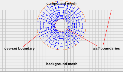
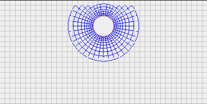
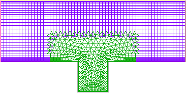
Figure 6.56: Overset Component and Background Mesh shows a simplified mesh for a simulation of flow over a cylinder in a duct. The mesh consists of two parts—a background mesh representing the duct and a separate component mesh around the cylinder. The case is set up in Fluent as an overset case by specifying the outer boundary of the cylinder mesh as overset (boundary type), and by creating an overset interface containing the two cell zones. With these two steps complete, Fluent automatically establishes the necessary connectivity between the meshes when the flow is initialized. In this process, cells that fall outside the computational domain are classified as dead cells. The cells where the flow equations are solved are referred to as solve cells. Receptor cells receive data interpolated from another mesh. The donor cells—the cells where the receptors get their data—are a subset of the solve cells. For the above case, Figure 6.57: Solve Cells After Initialization shows the solve cells of the mesh after the flow is initialized. Note that in parallel, you can print partition statistics to get information about some of the cell classifications, as described in Interpreting Partition Statistics.
There is no limit on the number of cell zones that can be paired in an overset interface. Fluent classifies the cell zones in an overset interface as either background or component:
Background zones are the cell zones that make up the background mesh of the computational domain. Background zones cannot have overset boundaries.
Component zones overlay background zones and have overset boundaries near where they connect to the background and other component zones. If multiple component zones are connected, at least one of these zones needs to have an overset boundary.
All cell types generally supported in Fluent are supported with overset meshing, including polyhedral cells in 3D. The different zones paired in an overset interface can have different element types or can have mixed element types.
Overset meshing in Fluent is compatible with mesh adaption. The mesh zones of an overset interface can be locally adapted using all available adaption tools.
Overset meshing can be used for steady-state or transient solutions. Note that for steady-state cases in parallel that use the default Metis partitioning, Ansys Fluent will automatically repartition overset meshes when the solution is initialized or data is read; a model-weighted partitioning that is designed for optimal performance is used.
There are a multitude of configurations that can be constructed by superposing background and component meshes in an overset interface. Fluent analyzes the topology of an interface with minimal user input, which requires that the superposed meshes adhere to some topological constraints.
A case can have multiple overset interfaces, but a cell zone can only belong to a single interface. That is, interfaces cannot share component or background meshes. It is always possible to have a single overset interface for an entire model. However, it is more efficient to declare multiple interfaces if the zonal topology allows it. Only including cell zones that are absolutely required in an interface also increases efficiency.
In general, most overset interfaces will have at least one background and one component mesh. However, Ansys Fluent also allows you to set up overset interfaces that have no background mesh and consist only of two or more component meshes.
An overset interface can contain multiple component and background meshes, provided that the background meshes do not intersect each other.
Currently, non-conformal interfaces are not fully compatible with overset meshing. Non-conformal mesh interfaces are permissible inside overset cell zones if the mesh interface boundaries do not spatially overlap with where the active overset interface lies. The proximity between the mesh interfaces and overset interfaces is checked during initialization and when the overset interfaces are updated. A warning is issued and the mesh check will fail if not enough separation is detected between the interfaces.
The component meshes of an overset interface are allowed to overlap arbitrarily and multiple component meshes can be combined to create an object of interest. However, an important topological constraint is that physical boundary zones (wall, inlet, outlet, symmetry, and so on) are not allowed to intersect each other. That is, a wall boundary cannot cross another wall boundary. For example, in the model shown in Figure 6.56: Overset Component and Background Mesh, the component mesh cannot be placed such that its wall boundary zone intersects with the wall of the background mesh.
Overset boundaries can intersect with other overset boundaries and with physical boundaries. In Figure 6.56: Overset Component and Background Mesh the overset boundary of the component mesh extends outside of the intended computational domain, crossing the wall boundary of the background mesh—this is allowed. Figure 6.58: Valid Overset Meshes with Components in Close Proximity shows a valid configuration of three cylinders in proximity (none of the physical boundaries intersect with other physical boundaries).
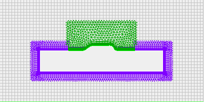
Physical boundary zones are allowed to overlap, that is, a wall boundary (or parts of a wall boundary) can be coincident with another wall boundary, as long as they do not cross. This powerful functionality lets you build a body from overlapping parts or modify a body by adding parts. Figure 6.59: Second Component Modifying Existing Body shows an overset configuration where a second component mesh is added to an existing body to modify its shape. Fluent analyzes and automatically detects the overlapping boundaries (walls in this case) of the different meshes in an overset interface, when deciding which cells are solve cells and which cells are dead cells.
Note that part of the wall boundary of mesh A lays on top of part of the wall boundary of mesh B, overlapping it, but the walls do not cross or intersect.
Figure 6.60: Existing Body Modification After Initialization shows the solve cells of the mesh after the flow field is initialized.
The previous example shows a case where physical boundaries overlap between two component meshes. Overlapping boundaries can also exist between component and background meshes.
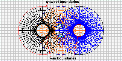
If a body can only be built from components that have intersecting boundaries, then you must use a collar mesh to properly connect them. A collar mesh is an additional component mesh that bridges the intersecting physical boundaries, essentially transforming the intersection problem (not allowed) into a problem of overlapping boundaries (allowed). Figure 6.61: Multiple Components Bridged by Collars Meshes shows an overset interface consisting of two component meshes that have intersecting wall boundaries. Two collar meshes (labeled C and D) are manually created to correctly define the connectivity where the wall boundaries of the original component meshes (labeled A and B) intersect. The wall boundaries of meshes C and D overlap with the wall boundaries of meshes A and B.
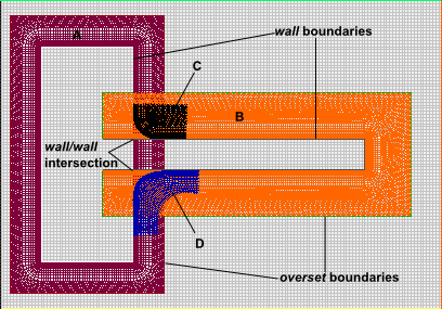
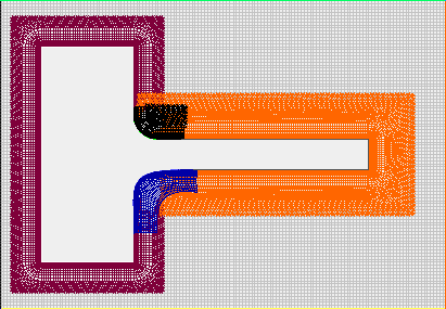
Figure 6.62: Multiple Components with Collar Meshes Initialized shows the resulting solve cells after the flow is initialized. The collar meshes act as fillet meshes that place the actual boundary intersections into the interior of the body and outside of the fluid domain.
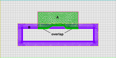
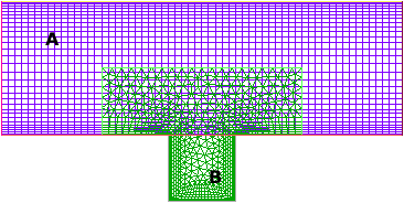
Special considerations are required when you intend to add a fluid region that expands the bounds of an existing region, as shown in Figure 6.63: Adding Fluid to a Region Using Cut Control. In this example, a duct (A) is modified by adding a cavity (B). The boundaries of the two meshes intersect, and by default the lower boundary of the duct would cut off the added cavity. In order to avoid this, you need to use cut control to specify that the duct wall is not cutting the cavity cell zone, and, similarly, that the cavity boundary is not cutting into the duct cell zone. See Hole Cutting Control for details on the available cut controls. The resulting mesh for the duct / cavity example after initialization is shown in Figure 6.64: Cut Controlled Region After Initialization.
Baffles (coupled walls) are permissible in overset meshing—both in background and component meshes.
When an overset interface is initialized, there are three main steps that Fluent completes to establish connectivity between the participating zones:
Hole cutting is the process by which cells lying outside of the flow region (that is, inside bodies and outside of the computational domain) are marked as dead cells. This is achieved by marking all the cells that are cut by physical boundary zones (wall, inlet, outlet, symmetry, and so on), and marking seed cells determined to lie outside the flow region for subsequent flood filling of dead cells. The result of this flood filling is a valid overset mesh with maximum mesh overlap.
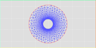
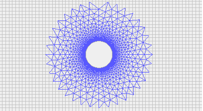
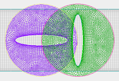
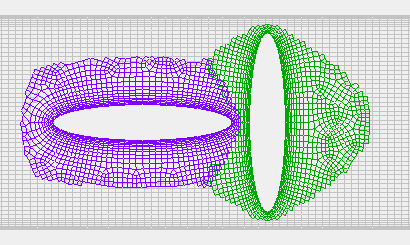
Figure 6.65: Overset Component and Background Meshes Before Hole Cutting and Figure 6.66: Overset Component and Background Meshes After Hole Cutting show an overset mesh before and after hole cutting. All of the background cells that are bounded or cut by the cylinder wall are classified as dead during hole cutting. The maximum overlap mesh shown in Figure 6.66: Overset Component and Background Meshes After Hole Cutting is a valid overset mesh, however, it may not be ideal. An overly large overlap between component and background meshes is computationally inefficient (the equations are solved in more cells than are necessary). Additionally, the cell sizes of the overlapping meshes may vary greatly—this affects the data interpolation and is detrimental to solution quality. Ideally meshes should transition in regions of similar resolution.
By default all boundary zones (other than overset boundaries) cut all other cell zones and mark dead cells. If this is not the desired behavior (see Overset Topologies), you can manually specify that a boundary zone does not cut certain cell zones. This optional cut control is available using the following text command:
define → overset-interfaces
→ cut-control →
add
A component mesh with only overset boundaries (for example, a refinement mesh zone overlaying other zones) will cut into other mesh zones at its center and mark a single dead cell (cut seed) in the overlaying mesh zones. This acts as a pilot hole that is then enlarged during the overlap minimization. In cases where all cut boundaries of a component mesh are overlapping with other boundaries, you can force cut seeds in all component zones using the following text command:
define → overset-interfaces
→ cut-control →
cut-seeds →
cut-seeds-for-all-component-zones?
Cut seeds are automatically enabled for all component zones when a cut control is added.
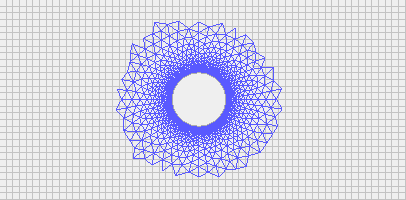
Overlap minimization is used to minimize mesh overlap among different component and background meshes by converting additional solve cells into receptor cells and turning unnecessary receptors into dead cells. During this process, a solve cell is turned into a receptor cell if the cell can find a suitable donor cell with higher donor priority. By default, smaller cells have a higher donor priority. Thus, in mesh overlap areas, without additional user input the solver attempts to obtain the solution on the finest local mesh. The resulting mesh interface moves to an area where the meshes are more comparable in cell size, leading to better solution quality. Figure 6.67: Overset Component and Background Meshes After Overlap Minimization shows the cylinder case from the previous figure after the overlap minimization step.
Note that overlap minimization is not literally minimizing the mesh overlap. The overlap minimization is based on a flood filling of receptor cells, wherever suitable solve cells with higher donor priority can be found. The resulting actual mesh overlap depends on the local donor priority distribution.
Also note that with overlap minimization, data interpolation between cell zones does not necessarily occur at the overset boundaries. The purpose of specifying an overset boundary is primarily to specify that overset mesh coupling should happen, and not where it should occur.
You have the option to specify different donor priority methods in order to control
the location of the overset interface. The text user interface command
define/overset-interfaces/options/donor-priority-method allows
you to specify that the donor priority is based either on the cell size (proportional to
the inverse of the cell volume) or the boundary distance (proportional to the inverse of
the distance to the closest boundary). Overlap minimization with donor priority based on
cell size (default) works best if the component mesh resolution is fine near walls and
increases away from walls, to spacings similar to—or larger than—the
background mesh (see Figure 6.65: Overset Component and Background Meshes Before Hole Cutting for an example of
this type of mesh). If the overlapping meshes have uniform and nearly identical
resolutions, then overlap minimization based on cell size will not reduce the overlap and
a donor priority based on the boundary distance should be used instead. The following two
figures illustrate an overset mesh before and after initialization where a donor priority
based on boundary distance is used. Note that for the evaluation of donor priorities based
on boundary distance, all boundaries (including inlets, outlets, and so on) are used for
the distance evaluation.
You have the option for additional control over the overlap minimization process by
assigning grid priorities to component and background meshes, using the text user
interface command define/overset-interfaces/grid-priorities.
Meshes (that is, cell zones) with higher grid priorities are favored during the
minimization process, irrespective of the local cell donor priority. If two cell zones
have the same grid priority, then the cell donor priorities are used for the overlap
minimization. For example, by assigning a higher grid priority to a coarser mesh, you can
force Fluent to minimize the finer mesh and obtain the solution on the coarser mesh,
even if the donor priority is based on cell size. Using grid priorities, similar to using
donor priority based on boundary distance, is helpful if local mesh distributions are
irregular, and produce overlap regions that are irregular as well. Note that the grid
priorities take precedence over the donor priorities.
You have the option of disabling overlap minimization by using the text command
define/overset-interfaces/options/minimize-overlap?. This
command is only available globally and applies to all overset interfaces in the
domain.
The donor search is the final step in establishing the domain connectivity. Fluent searches other meshes for valid solve cells for each receptor. The solve cell containing the cell centroid of the receptor cell, along with its connected solve cells, are used as donor candidates for a given receptor. Each receptor must have at least one valid donor cell.
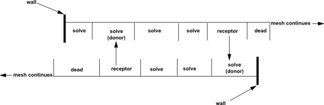
There must be four or more cells in the overlap of both meshes to ensure a successful donor search. The receptor cells, which form the fringe layer of a mesh zone, must overlap sufficiently with the opposite mesh, such that they find valid solve cells as donors. For an example of valid mesh overlap, see Figure 6.70: Valid Overlap.
Topology detection of overset interfaces in Fluent is automatic and does not require user input. However, for it to work well, it requires that the provided meshes are of sufficient quality, particularly when dealing with meshes that have overlapping boundaries.
Overset meshes are built from parts that can be meshed independently, which can lead people to think of this as a much simpler process for mesh generation. This is not always the case, as considerable thought is often required to generate good meshes for the individual components to avoid problems during overset interface initialization.
If you are faced with issues during the initialization of an overset interface, there is most often no recovery without making changes to the mesh. You must analyze the cause of the issue, using the available postprocessing and diagnostic tools, and improve the mesh before the simulation can continue.
When diagnosing overset interface failures, it can be convenient to use the text
commands define/overset-interfaces/intersect and
define/overset-interfaces/clear (available after enabling the
expert tools available under
define/overset-interfaces/options/expert?) to execute and clear
the hole cutting without having to initialize the solution.
The issues most often encountered are:
These are the issues that can cause problems with flood filling:
Flood filling of dead cells will fail if Fluent inadvertently identifies seed cells inside of the fluid zone instead of outside. This can occur as a result of complexities in the topology or geometry of the boundary zones, or because of mesh resolution issues. It manifests itself as an entire fluid region, or a complete cell zone, being marked as dead.
This issue can be diagnosed by using the list command with the overset verbosity set
to 1 (see Overset Interface Listing).
You can use the TUI command
define/overset-interfaces/debug-hole-cut (available after
enabling the expert tools available under
define/overset-interfaces/options/expert?) to identify the
problematic seed cells. This command allows you to execute the hole cutting process on a
specific overset interface and mark dead and seed cells.
When the flood fill option of the debug command is disabled, it will create two
registers with dead cells and seed cells which you can then display using the
define/overset-interface/display-cells text command. The dead
marks show the cells cut by the physical boundary zones. The seed cells (mark0 register)
show the cell candidates that will be used for flood filling.
If the flood fill option of the debug command is enabled, Fluent will then also create a register of the seed cells from where flood filling actually started (mark1 register). If flood filling fails, displaying these mark1 cells is the most efficient way to detect the problematic locations in the model.
It is critical that all the seed cells are located inside bodies or outside of the computational domain. If there is a seed cell in the fluid region, it will cause a flood fill failure. It is not possible to recover from flood filling failure without making changes to the model.
If no bad seed cells are found, as described in Incorrect Seed Cells, and there are overlapping boundaries, it is likely that the overlapping boundaries do not match sufficiently and the flood filling of dead cells leaks from the inside of the body to the outside. As a result, a complete cell zone can disappear, due to having only dead cells. The permissible tolerance between overlapping boundary zones is at most one cell-size in the wall normal direction. This can be restrictive when dealing with prismatic boundary layer meshes with high cell aspect ratios at the wall. If your model suffers from this leakage, you generally need to improve the quality of the mesh, by making the overlapping boundary zones match better.
If a receptor cell cannot find a valid donor cell, then it becomes an orphan cell. The presence of orphan cells generally indicates that there is insufficient overlap between meshes or that the mesh resolutions do not match well. As a result, the receptors are either finding no candidate donor cells, or invalid candidates (dead or receptor cells).
Orphan cells can be an issue when walls of different meshes are in proximity. You must have at least four cells in a gap, such as the ones between the walls in Figure 6.58: Valid Overset Meshes with Components in Close Proximity, in order to have a good connection between the meshes—otherwise orphan cells are created. When a receptor overlays another receptor, it becomes an orphan.
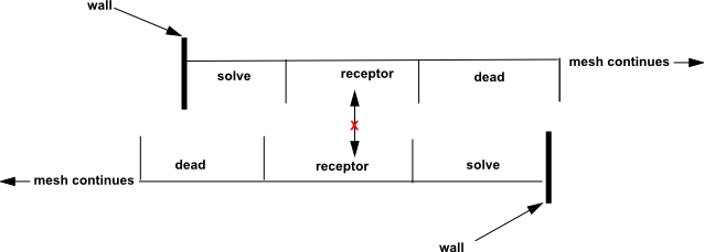
See Figure 6.71: Invalid Overlap Creating Orphans for an example of insufficient overlap causing the creation of orphan cells. For information on visualizing orphan cells, see Postprocessing Overset Meshes. Figure 6.70: Valid Overlap shows meshes overlapping sufficiently to avoid the creation of orphan cells.
You can mark the orphan cells, as described in Overset Cell Marks, which will likely indicate where the mesh overlap must be increased. Sometimes, increasing the mesh resolution can lead to a sufficient increase in mesh overlap. If mesh resolution is the issue, you can also use local mesh adaption, along with mesh modification, to refine the mesh. Most often the mesh requiring adaption is the mesh where the orphan should find its donors, and not the mesh zone containing the orphan. For details on overset-specific adaption tools in Fluent, see Overset Mesh Adaption.
If the presence of orphan cells in the simulation is unavoidable and you proceed with a calculation, by default the solver applies a numerical treatment that attempts to assign reasonable values to the orphan cells. This treatment has been found to prevent divergence in some instances, allowing the solution to proceed; however, the orphan cell treatment does not guarantee the solution quality and robustness a priori. The success of this treatment is case dependent, and difficult to predict based on orphan cell counts. It is therefore highly recommended that you make every effort to eliminate orphan cells by modifying the mesh, as described previously.
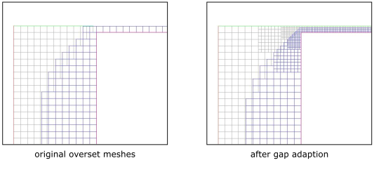
Fluent has functionality that allows you to attempt to remove orphan cells, reduce size mismatches between donor and receptor cells, and/or increase the mesh resolution in gaps as needed (in order to prevent the creation of orphan cells) by locally refining the mesh. These are overset-specific adaption tools that analyze the initialized overset interface and can perform marking and adaption of cells in a single step.
It is important to note that there are different reasons for the existence of orphan cells, and that not all orphans can be removed by locally refining the mesh. Overset adaption will proceed iteratively, up to a maximum of five adaption cycles: cells are marked at the start of each cycle, and by default two sweeps of adaption are applied during each cycle. Multiple adaption sweeps are performed for a given set of adaption markings in order to reduce the time taken for the adaption process. The overset interface needs to be reestablished after each adaption cycle, which can be computationally costly. In cases where mesh resolution is the reason for orphans, this adaption process should effectively improve the mesh and reduce the orphan count.
Overset mesh adaption can be used to improve the mesh either manually on demand, or automatically for moving and dynamic mesh simulations. If automatic overset adaption is enabled, then the mesh is marked and adapted automatically at every time step after the mesh update. Since it is computationally costly to establish the overset connectivity at the end of each adaption cycle, Fluent performs only a single cycle during automatic overset adaption. Thus, a single automatic overset adaption step may not be as thorough in removing orphan cells as an instance of manual adaption; however, automatic overset adaption will be executed at every time step if orphan cells persist.
For each orphan, all of the cells in the overlapping meshes that bound the orphan's cell centroid are marked for adaption; by default, an additional buffer layer of cells surrounding those bounding cells are also marked. The mesh zone that contains the orphan cell is not marked for adaption.
Excessively large donor cells are marked for adaption if the ratio of the donor cell
volume ( ) divided by its smallest receptor cell volume (
 ) exceeds a limit. This limit is controlled by a maximum length scale
ratio
) exceeds a limit. This limit is controlled by a maximum length scale
ratio  . Donor cells with a
  value greater than
  in 3D and greater than
  in 2D are marked for adaption. The default value for
  is 3.
is 3.
After initialization, the value for  can be postprocessed by selecting the Overset Donor Size
Ratio field variable (under the Mesh... category).
can be postprocessed by selecting the Overset Donor Size
Ratio field variable (under the Mesh... category).
For overset meshes, it is recommended that the gaps between walls are resolved by a minimum of 4 cells, in order to create a valid overset interface and prevent the creation of orphan cells. You can specify that the cells in gaps with a resolution that is less than this recommendation (or another gap resolution value of your choice) are marked for adaption, so that any subsequent overset adaption (manual or automatic) increases the resolution to meet or exceed the gap resolution value. Note that marking cells for gap adaption is not enabled by default, but can be enabled as described in Overset Adaption Controls.
Overset adaption can be applied manually on demand in order to improve the mesh. Typically it is used in steady simulations or simulations without mesh motion.
The overset mesh is marked and adapted in a single step using the following text command:
define →
overset-interfaces → adapt
→ adapt-mesh
You can perform just the marking step for overset adaption by
entering the following text command:
define/overset-interfaces/adapt/mark-adaption. Note that it is
not necessary to perform this marking step before using the command to adapt; the purpose
of such marking is primarily to verify the adaption parameters and evaluate whether they
need to be changed. The text command to mark for adaption will mark cells (mark0 for
orphan adaption, size adaption, and gap adaption, and mark1 for coarsening), so that you
can then create cell registers and thereby postprocess them as described in Overset Cell Marks. Note that mark0 and mark1 are only available
after enabling the expert tools through the following text command:
define/overset-interfaces/options/expert?.
You can use the following text command to set a verbosity level
of 2 if you want to print the number of cells marked for
refinement in the console when the overset mesh is adapted:
define/overset-interfaces/options/verbosity.
With moving and dynamic mesh simulations, it can be difficult to create an initial mesh that meets all of the needs throughout the simulation while also being computationally efficient. Rather than refining the initial mesh in regions that only require such refinement temporarily, it can be preferable to use automatic overset adaption so that Fluent analyzes the mesh at every time step and then refines or coarsens the cells as required; the goal is to remove orphans and/or reduce size mismatches between donor and receptor cells.
To enable automatic overset adaption, you can use the Automatic Mesh Adaption Dialog Box as described in Overset Adaption, or you can use the following text command:
define →
overset-interfaces → adapt
→ set → automatic?
Automatic overset adaption is fully compatible with conventional automatic mesh adaption, such as when it is used to more accurately track Volume of Fluid (VOF) interfaces (as described in VOF Adaption). The two adaption methods can be enabled at the same time, and will not interfere with each other.
If the default settings for overset adaption are not suitable for your case, you can revise them using the text commands in the following menu:
define →
overset-interfaces → adapt
→ set
The text commands in this menu include:
-
automatic? Enables/disables the option to automatically adapt overset meshes during the calculation, to remove orphans, reduce size mismatches between donor and receptor cells, and/or increase the mesh resolution in gaps as needed (in order to prevent the creation of orphan cells). This option is disabled by default.
-
maximum-refinement-level Sets the maximum level of refinement during overset adaption, in conjunction with the value set using the
mesh/adapt/set/maximum-refinement-leveltext command (the larger of the two values is used). This is set to 4 by default.-
mark-size? Enables/disables the option to adapt based on donor-receptor cell size differences.
-
length-ratio-max Sets the length scale ratio threshold used to determine which cells are marked for adaption based on donor-receptor cell size differences. This is set to 3 by default and is only available when
define/overset-interfaces/adapt/set/mark-size?is enabled.-
mark-orphans? Enables/disables the option to adapt for orphan reduction.
-
buffer-layers Sets the number of cell layers marked in addition to the cells marked for orphan adaption. This is set to 1 by default.
-
mark-fixed-orphans? Enables/disables the option to also adapt based on cells that are not actual orphans because they were fixed by accepting neighbor donors. This option is only available when
define/overset-interfaces/adapt/set/mark-orphans?is enabled.-
mark-gaps? Enables/disables the option to adapt under-resolved gaps in order to prevent the creation of orphan cells. This option is disabled by default.
-
gap-resolution Sets the target (minimum) gap resolution used when marking cells for gap adaption. This is set to 4 by default and is only available when
define/overset-interfaces/adapt/set/mark-gaps?is enabled.-
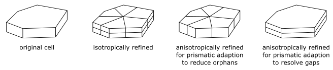
prismatic? Enables/disables the option to use prismatic adaption for the cells that are refined in order to reduce orphans and/or better resolve gaps. Instead of being isotropically refined, these cells will be anisotropically refined (that is, they will not be split on particular edges), in order to reduce the resulting cell count. This adaption option is referred to as "prismatic", because it is only available for 3D prismatic cells that are deemed suitable. For orphan adaption, the goal is to produce cells that have a lower aspect ratio; for gap adaption, the goal is to produce a mesh resolution that is suitable for boundary layers near walls.
-
mark-coarsening? Enables/disables the option to coarsen the mesh if mesh refinement is no longer needed. This option is enabled by default.
-
adaption-sweeps Sets the number of sweeps of adaption applied during each adaption cycle. This is set to 2 by default.
Receptor and donor cell sizes should be comparable to ensure that interpolation errors are minimized. You can adapt the mesh to reduce the mismatch between donors and receptors (see Overset Mesh Adaption).
You must have a minimum of four cells in a gap to create a valid overset interface, but a higher number is recommended to ensure robust coupling between meshes and to prevent the creation of orphan cells (see Figure 6.71: Invalid Overlap Creating Orphans and Figure 6.70: Valid Overlap). You can adapt the mesh to refine under-resolved gaps (see Overset Mesh Adaption).
When using the pressure-based solver, the default pressure-velocity coupling scheme for overset meshes is Coupled, and this is generally recommended. However, for transient simulations using time step sizes comparable to CFL limits, the greater computational efficiency of a segregated scheme (SIMPLE, SIMPLEC, or PISO) can help in reducing the total simulation time. Note that as you employ larger time step sizes with respect to CFL limits, the tighter pressure-velocity coupling offered by the default Coupled scheme makes it the preferred scheme for such cases. For details on these schemes, see Choosing the Pressure-Velocity Coupling Method.
The use of standard initialization with defaults computed from all zones has been found to be useful for turbulent simulations starting from quiescent flow, especially for the segregated pressure-velocity coupling schemes.
It is recommended that you start transient simulations from a converged steady-state solution.
If you are experiencing startup issues with a steady-state case, it is recommended that you ramp-up to the final boundary conditions. For example, you can begin with a lower inlet velocity and a higher viscosity to establish flow, before increasing to the target velocity and the desired final material properties.
When using automatic time step calculation for the pseudo time method (with the global time step method selected), it is recommended that you use the user-specified length scale method.
If you replace a zone that is part of an overset interface, you should either reinitialize the solution or patch the solution on the replaced zone(s) before continuing with the calculation.
It is recommended that you use the double-precision solver for overset mesh simulations.
Closed domain cases are defined as setups that do not have a flow inlet or outlet boundary; this type of setup is not supported with overset meshing if the working fluid is incompressible. If such a setup is unavoidable, creating a small pressure-outlet boundary far away from the region of interest is recommended before attempting to run the case using overset meshes.
For dynamic and sliding mesh cases, note the following:
The ideal time step size should be chosen such that the relative mesh motion does not exceed the length of the smallest cell at the overset interface for a given time step for first order in time, and half that length for second order in time. The mesh length used for calculating the time step size should be restricted to cells in the overset overlap region. This ensures a more gradual evolution of the overset interface with the motion and is recommended for better accuracy and stability.
With Volume of Fluid (VOF) simulations using second order in time, the solution strategies for multiphase modeling could be beneficial in improving the stability of your simulations (see VOF Solution Stability Controls). When using a large CFL value (that is, greater than 1), it is recommended that you run with first order in time to ensure the simulations remain stable.
In general, the motion of the overset interface may change the status for individual cells from dead to receptor or solve, and vice versa. The exact instances depend on the relative mesh sizes of the moving cell zones participating in the overset interface, the magnitude of the relative mesh velocity, and the time step size. There is currently no mechanism to eliminate this type of cell status change for general cases.
While the solver is capable of handling the cell status change, it is recommended that you actively monitor these instances by setting the overset mesh verbosity to 1 using the
define/overset-interface/options/verbositytext command. With such a verbosity, the solver reports the instances of dead to solve cells in the console. Keeping these to a minimum is highly recommended for better accuracy and stability.Do not have large variations in mesh resolution in the motion path that could trigger large changes in the overset interface as the motion proceeds. The use of grid priorities can minimize large variations in the overset interface.
When using an overset mesh to simulate flow through narrow gaps that open or close over time (such as in a valve or a rotary pump), you can use the gap model to block or decelerate the flow when the gaps are closed (as described in Controlling Flow in Narrow Gaps for Valves and Pumps).
You can specify that the overset interfaces use either the least squares interpolation method (the default) or the inverse distance interpolation method by using the following text command.
solve → set →
overset → interpolation-method
When the porous zone option is enabled with an overset mesh, it is
recommended that you use the default least squares overset interpolation method, especially
if you have a porous zone that overlaps with another porous zone. If you need to use the
inverse distance interpolation method, you may also need to use pressure interpolation
schemes other than second order, as well as enable the use of high-order pressure
extrapolation at the overset interface (available through the following text command:
solve/set/overset/high-order-pressure? yes). This improves the
accuracy of the pressure gradients at the overset interface, which is vital for predicting
the pressure drop and flow in the porous zone.
Overset meshing has the following limitations and compatibilities:
Overset meshing currently has the following limitations:
Overset interfaces cannot contain solid cell zones.
Non-conformal mesh interfaces inside overset cell zones are only permitted if the mesh interfaces do not spatially overlap with the cells where the overset interfaces lie.
Component zones cannot have periodic boundary conditions.
Background zones cannot have overset boundaries.
Component mesh boundaries cannot overlap with coupled walls.
FMG initialization is not available.
The FAS multigrid scheme is not used.
Implicit residual smoothing cannot be enabled.
Overset meshing is not supported for incompressible flows in a closed domain.
The use of node weights for node-based gradients in postprocessing is not available for cases with overset meshes.
Overset meshing is not compatible with the Coupled Level Set + VOF hybrid model.
The turbulence models that are supported with overset meshing (listed in the section that follows) cannot be used in combination with Scale-Resolving Simulation (SRS) models / options.
When using an overset mesh with the DPM model:
The High-Res Tracking option must be enabled
Wall film particles cannot move between different overset meshes
Overset meshing is compatible with the transient and steady-state solvers. Both laminar and turbulent flow regimes with heat transfer are allowed as well as single phase flows, and Volume of Fluid (VOF) and mixture multiphase flows. These applications are valid with overset for the listed solver options and configurations. Unless otherwise specified, consider all other solver features and models to be unsupported.
Supported Options and Models:
Pressure-based solver using:
2D (planar and axisymmetric) and 3D flows in the absolute velocity formulation
Compressible flows
Cell-based gradient methods: Green-Gauss Cell Based and Least Squares Cell Based
All pressure interpolation schemes
First-order and second-order spatial schemes
SIMPLE, SIMPLEC, PISO, Fractional Step, and Coupled schemes for pressure-velocity coupling
All mass flux types (Rhie-Chow: distance based or Rhie-Chow: momentum based)
A pseudo time method
First-order, second-order, and (if available) bounded second-order transient formulations
The Non-Iterative Time Advancement (NITA) option
The hybrid NITA option (for cases that involve the Volume of Fluid model)
Density-based solver using:
2D (planar and axisymmetric) and 3D flows in the absolute velocity formulation
Compressible flows
Cell-based gradient methods: Green-Gauss Cell Based and Least Squares Cell Based
All convective flux types (Roe-FDS, AUSM, and Low Diffusion Roe-FDS)
First-order and second-order spatial schemes
A pseudo time method
First-order, second-order, and (if available) bounded second-order transient formulations
 -
- turbulence models: Standard, RNG, and Realizable
 -
- turbulence models: Standard, BSL, and SST
Spalart-Allmaras turbulence model
Laminar-turbulent transition models: Transition SST, Intermittency Transition, and Transition
 -
- -
-
Discrete Ordinates (DO) radiation model
Species transport model:
single-phase flow only
reactions must be disabled
VOF models:
Open channel flow and surface gravity waves
Cavitation and evaporation/condensation mass transfer
Mixture multiphase model:
Non-granular flows
Cavitation and evaporation/condensation mass transfer
Cavitation and evaporation/condensation mass transfer in VOF/Mixture multiphase applications
Non-granular flows in multiphase applications
Dynamic and sliding meshes with the first-order transient formulation
Gap model
User-defined scalars
User-defined functions (for information about overset-specific macros that can be useful when writing user-defined functions, see Overset Mesh Looping Macros in the Fluent Customization Manual)
All AMG options except for the Laplace Coarsening option (for the scalar or coupled parameters)
All boundary conditions are supported except for:
the following non-interior face zone boundary conditions: exhaust fan, inlet vent, intake fan, outflow, and outlet vent
the following interior face zone boundary conditions: fan, porous-jump, and radiator
Cell zone conditions
Source terms may only be defined on cell zones not participating in an overset interface
Fixed values may only be defined on cell zones not participating in an overset interface
Multiple Reference Frame (MRF) model
The porous zone option is supported with the superficial velocity formulation
Hybrid and standard initialization
An overset meshing solution may be obtained on any mesh type, including adapted meshes
Once you have read all of the related meshes into Fluent, use the following steps to setup an overset interface.
Change the boundary zones of component meshes to overset (boundary type), where needed.
Important: You must correctly specify the overset boundaries for all zones in an overset interface before creating the overset interface. (Once overset interfaces are created you cannot change any boundaries from overset to another type or from another type to overset.)
 Setup → Boundary
Conditions
Setup → Boundary
Conditions  <boundary>
→ Type → overset
<boundary>
→ Type → overset
The Overset Dialog Box will open, which you can use to revise the Zone Name.
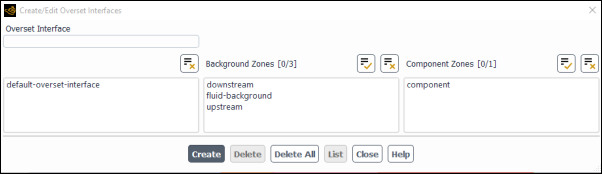
Create an overset interface between the cell zones that must be coupled. A case can have multiple interfaces. Each interface must have at least one background and one component mesh.
 Domain → Interfaces
→ Overset
Domain → Interfaces
→ Overset
Enter a name under Overset Interface.
Select the zones of the interface in the Background Zones and Component Zones selection lists. Ansys Fluent allows you to create interfaces that contain only component zones; in such cases, you do not select a background zone, but instead select two or more component zones.
Click .
(optional) If your overset case doesn’t have overlapping boundaries, and you don’t need Fluent to analyze the case for boundary overlaps, you can improve the overset performance by disabling overlap boundaries using the following text command:
define→overset-interfaces→options→overlap-boundaries?(optional) Use the text user interface for additional control over the hole cutting step of the interface initialization.
If certain boundary zones should not cut particular cell zones, use the
define/overset-interfaces/cut-control/addtext command to set up cut control.If component meshes have no boundaries that will cut a cell zone, you can use the
define/overset-interfaces/cut-control/cut-seeds/cut-seeds-for-all-component-zones?text command to ensure that all component zones get cut seeds (see Hole Cutting Control).
(optional) Use the text user interface for additional control over the overlap minimization of the overset interface. It can be helpful to revise the default settings if your overlapping meshes have uniform and nearly identical resolutions or if local mesh distributions are irregular, as this may improve the computational efficiency and/or the solution quality. See Overlap Minimization for details.
To specify whether the cell donor priorities used during minimization are based on the cell size or distance to the nearest boundary, use the following text command:
define→overset-interfaces→options→donor-priority-methodTo revise the grid priorities during minimization, use the following text command. The grid priority for each zone is an integer, and only the relative values between the zones matter.
define→overset-interfaces→grid-prioritiesTo disable overlap minimization entirely, use the following text command. This command is only available globally and applies to all overset interfaces in the domain.
define→overset-interfaces→options→minimize-overlap?
Note that these steps only define an overset interface. Hole cutting occurs during solution initialization.
If a case contains overset face zones, but no defined overset
interfaces, then Fluent creates a default interface with the name
default-overset-interface upon initialization. This default
overset interface contains all cell zones in the domain. If you know that some cell zones do
not need to be included in an overset interface, then you can increase the solution
performance by manually creating the interface and only including the relevant background
and component meshes.
Fluent has several overset-specific postprocessing tools to help you analyze/understand the domain connectivity. These tools are only available after the flow field is initialized and the domain connectivity is established.
You can either visualize the complete mesh or just the active cells. If the Overset option is enabled in the Mesh Display dialog box, by default only solve cells are shown. Disabling the Overset option displays the complete surfaces.
![]() Domain → Mesh
→ Display
Domain → Mesh
→ Display
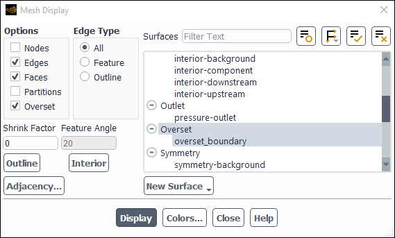
You have the option to have receptor cells displayed along with the solve cells when
Overset is selected. You can enable this option via the TUI command
define/overset-interfaces/options/render-receptor-cells?.
Note:
When displaying contours of postprocessing quantities, dead cell values are never shown, regardless of whether or not Overset is enabled in the Mesh Display dialog box.
You may notice a z-fighting effect when displaying overset meshes, particularly when coloring the mesh by ID. This occurs due to the nature of overset meshes, where two meshes are coincident and the rendering tool is conflicted in determining which color to display.
There is an Overset Cell Type function available in the Cell Info... category in the Contours Dialog Box. The integer function value depends on the overset cell type:
|
Cell Type |
Integer Function Value |
|
donor |
2 |
|
solve |
1 |
|
receptor |
0 |
|
orphan |
–1 |
|
dead |
–2 |
This field function is also available in the Contours dialog box.
![]() Results → Graphics
→ Contours → New...
Results → Graphics
→ Contours → New...
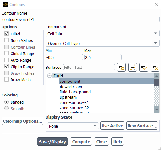
Select Cell Info... and Overset Cell Type from the Contours of drop-down lists.
Choose the surfaces containing the overset cells you want to visualize and click .
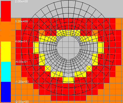
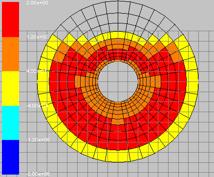
Figure 6.75: Contours of Overset Cell Type: Background Mesh and Figure 6.76: Contours of Overset Cell Type: Component Mesh display a background mesh and component mesh (sequentially) of Overset Cell Type for the cylinder problem shown in Figure 6.56: Overset Component and Background Mesh.
Note: If you want to display orphan cells, then you must enable the TUI command
define/overset-interfaces/options/render-receptor-cells?.
If the expert options are enabled under
define/overset-interfaces/options/expert?, then you can also
choose to display Overset Donor Count and Overset Receptor
Count under Cell Info…. The Overset
Donor Count is filled for each receptor and shows the number of donors.
Similarly, the Overset Receptor Count is filled for donor cells and
shows the number of receptors that are referencing the donors.
Note that the donor counts reported are the maximum number of donors available for the data interpolation. The actual number of donors used by the solver may be less.
It can be difficult to interpret contours of overset cells in 3D. Often, it is more illustrative to mark a certain type of overset cells and display these marked cells.
Using the text command
define/overset-interfaces/mark-cells you can mark cells of
specified overset cell type (solve, receptor, donor, orphan, or dead), either globally or
on a single cell zone. This command automatically fills registers that can be displayed
using the define/overset-interfaces/display-cells text
command.
Use the text command define/overset-interfaces/list to print
overset interface related information to the console. If the overset verbosity,
define/overset-interfaces/options/verbosity, is set to
1, then counts of each overset cell type are printed per cell
zone as well.
Volume integrals are taken over all solve cells in the domain. This results in double counting where solve cells overlap, leading to errors in volume integrals on overset meshes.
Similarly, surface integrals, including force and moment reports, will include errors when taken on surfaces created for postprocessing (such as plane surfaces or rake surfaces) in regions where solve cells or boundary zones overlap. If surface integrals are taken on boundary zones rather than created surfaces and/or in a region without overlap, then the surface integrals are exact.
Important: Errors in integral evaluations scale with the size of the overlap.
When writing overset case files, it is recommended that you use the default Common
Fluids Format (CFF), as in this format the overset domain connectivity is saved in the
.cas.h5 file. This makes it unnecessary to reestablish the domain
connectivity when reading an overset case into a new session, as is the case with legacy
case files (.cas). It also guarantees an identical connectivity
when a case is read on a different number of compute nodes.
When you write an overset case file in CFF and the case has not yet been initialized,
Ansys Fluent will by default establish the domain connectivity prior to writing the file. This
can be disabled using the
define/overset-interfaces/options/update-before-case-write? text
command, which is available after you enable the expert tools using the
define/overset-interfaces/options/expert? command.