


In Ansys Fluent, you can generate graphics displays showing meshes, contours, profiles, vectors, pathlines, and scenes. Some graphics are generated using variables that are plotted directly from the Ansys Fluent data file once the file has been read. The variables listed in the data file depend on the models active at the time the file is written. Variables that are required by the solver, based on the current model settings, but are missing from the data file are set to their default values. For those missing variables, one iteration should be performed in order to obtain the required values for generating the plot. A complete list of variables stored in the data file is available in (xfile.h) and can be accessed as stated in Data Sections. The following sections describe how to create these plots. (Generation of histogram and XY plots is discussed in Histogram and XY Plots.)
Important: If your model includes a discrete phase, you can also display the particle trajectories, as described in Displaying of Trajectories.
Note: There are two kinds of graphics objects—those whose settings are saved with the case file for reuse during the simulation, and those that are not. Persistent graphics objects (saved with the case file) are accessed by clicking New....
![]() Results → Graphics
→ Contours
→ New...
Results → Graphics
→ Contours
→ New...
Non-persistent objects (typically created by clicking Edit...) are deprecated and hidden from the user interface by default. To bring back this functionality, enable Expose legacy non-persistent graphics in the Graphics branch of Preferences (accessed via File>Preferences...).
Remote Display: If graphics displays appear slow, it may be related to the graphics driver. Ensure
Display Power Management Signaling (DPMS) is enabled by entering the
xset -display :0 dpms force on command in the Xterm
window.
If glxgears is not working correctly (at least a few thousand frames per second), then you may require assistance from your IT team.
This section discusses the following topics:
- 40.1.1. Graphics Performance
- 40.1.2. Displaying the Mesh
- 40.1.3. Displaying Contours and Profiles
- 40.1.4. Displaying Vectors
- 40.1.5. Displaying Pathlines
- 40.1.6. Displaying Line Integral Convolutions (LICs)
- 40.1.7. Displaying a Scene
- 40.1.8. Displaying Results on a Sweep Surface
- 40.1.9. Hiding the Graphics Window Display
A number of factors can influence the graphics performance of your machine, including the model size and mesh type, the quality of your graphics card, what you are displaying (type of graphics object and number of surfaces being displayed), and your Fluent Preferences.
Using a modern graphics driver, such as OpenGL2 (Linux, Windows) or DX11 (Windows) will let you take full advantage of Fluent's graphical capabilities.
You can set preferences to automatically use the best graphics options for your case, or you can set them to optimize for appearance or performance. Refer to Optimizing Graphical Priorities for additional information.
![]() File
→ Preferences...
File
→ Preferences...
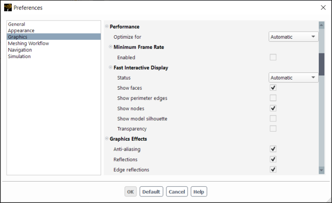
The Status of Fast Interactive Display indicates whether the strategically reduced display is invoked automatically based on the size of your model display (number of faces being displayed) and your machine's ability to display it, or if it is always on or always off.
You can specify what will be shown when the fast interactive reductions are invoked by enabling the desired options under Fast Interactive Display.
Note:
The first time your model is displayed with Show perimeter edges enabled, you may experience a delay in the interaction while Fluent generates the reduced display.
Graphics objects may partially or completely disappear during graphics window mouse interactions (such as zooming or panning). Disable Fast Interactive Display in Preferences to avoid this behavior.
Important: Fast Interactive Display options are not compatible with Minimum Frame Rate.
During the problem setup or when you are examining your solution, you may want to look at the mesh associated with certain surfaces. You can do the following:
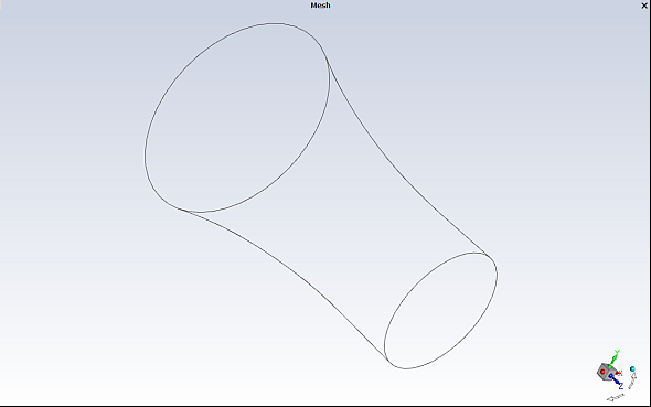
Display the outline of all or part of the domain, as shown in Figure 40.2: Outline Display.
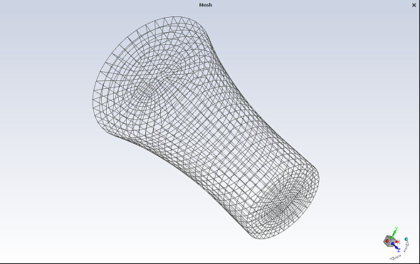
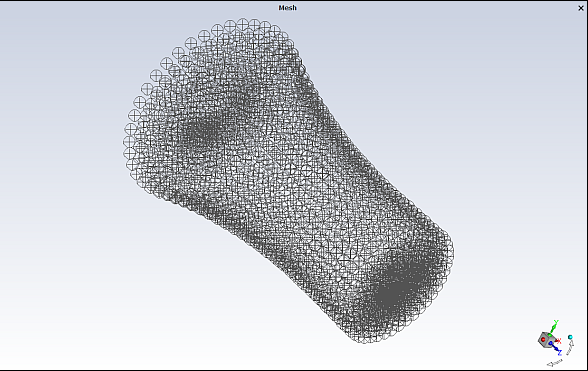
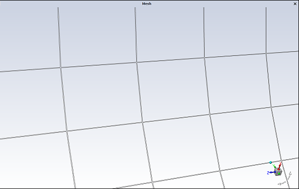
Draw the mesh lines (edges), as shown in Figure 40.3: Mesh Edge Display.
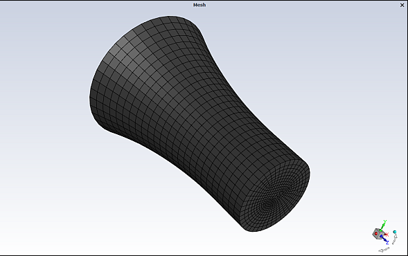
Draw the solid surfaces (filled meshes) for a 3D domain, as shown in Figure 40.4: Mesh Face (Filled Mesh) Display.
Note: You can control how reflective the surfaces appear using the Surface specularity for other surfaces field in the Appearance branch of . Values closer to 1 are more reflective, while those closer to 0 are less reflective.
Draw the nodes on the domain surfaces, as shown in Figure 40.5: Node Display.
Note: (Parallel Fluent sessions) Mesh displays with Edges enabled and either Feature or Outline selected will not show any partition lines by default. This default behavior is controlled by the Remove partition lines option in the Graphics branch of Preferences (accessed via File>Preferences...).
If it appears that your model is de-featured or faces are collapsed, try reducing the Partition line removal tolerance setting in Preferences. Conversely, if you are still seeing fragments of partition lines, try increasing the Partition line tolerance.
For information about displaying the mesh on a surface that sweeps through the domain, see Displaying Results on a Sweep Surface.
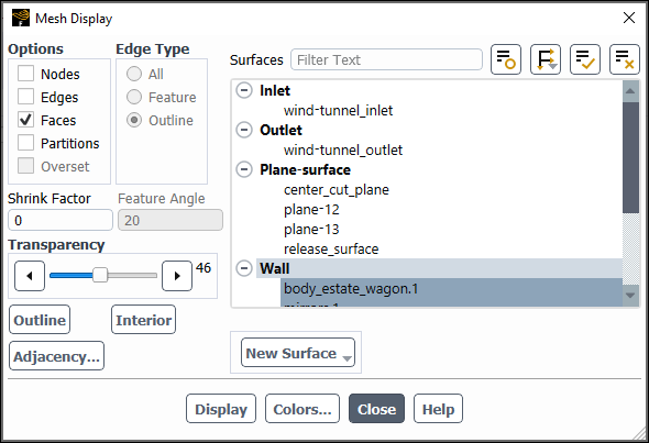
You can draw the mesh or outline for all or part of your domain using the Mesh Display Dialog Box (Figure 40.6: The Mesh Display Dialog Box).
![]() Results → Graphics
→ Mesh
Results → Graphics
→ Mesh
![]() New...
New...
The basic steps for generating a mesh or outline plot are as follows:
Choose the surfaces for which you want to display the mesh or outline in the Surfaces list.
If you want to select several surfaces of the same type, click
 and select Surface Type under
Group By, which organizes the surfaces in a
tree view that is grouped by surface type.
and select Surface Type under
Group By, which organizes the surfaces in a
tree view that is grouped by surface type.Another shortcut is to use the Filter Text entry box to filter the Surfaces list to show only the surfaces that match the pattern you enter. For additional information on using the Filter Text entry box, see Filter Text Entry Boxes.
Depending on what you want to draw, do one or more of the following:
To draw an outline of the selected surfaces (as in Figure 40.2: Outline Display), select Edges under Options and Outline under Edge Type. If you need more detail in the outline display of a complex geometry, see the description of the Feature option, below.
To draw the mesh edges (as in Figure 40.3: Mesh Edge Display), select Edges under Options and All under Edge Type.
Note: Mesh edges are disabled by default. You can enable Show model edges in the Appearance branch of Preferences (accessed via the File ribbon tab) to change the default behavior so that all new mesh objects you create will have mesh edges enabled.
To generate a filled-mesh display (as in Figure 40.4: Mesh Face (Filled Mesh) Display), select Faces under Options.
To draw the nodes on the selected surfaces (as in Figure 40.5: Node Display), select Nodes under Options.
Set any of the mesh and outline display options described in the following section.
Click Save/Display to draw the specified mesh or outline in the active graphics window.
To display filled meshes, with smoothly shaded display, enable lighting and select a lighting interpolation method other than Flat in the Display Options Dialog Box or the Lights Dialog Box.
If you display nodes, and you want to change the symbol representing the nodes, you can change the Point Symbol in the Display Options Dialog Box. See Modifying the Rendering Options for details.
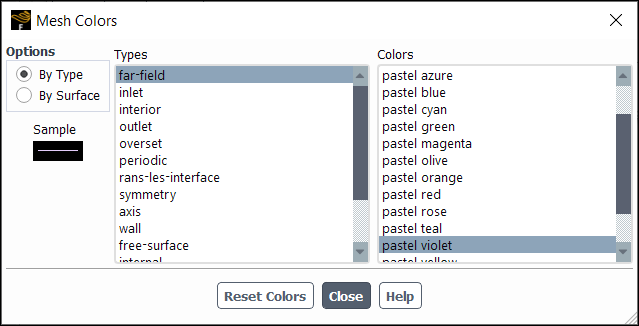
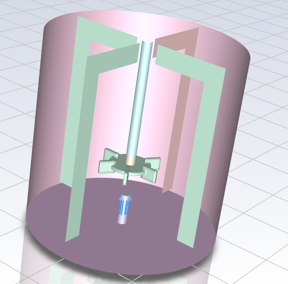
Ansys Fluent enables you to control the colors that are used to render the meshes for each zone type or surface. This capability can help you to understand mesh plots quickly and easily. Ansys Fluent offers two distinct color palettes that you can use to color the mesh: Classic and Pastel (Figure 40.12: Mesh Display with Pastel Color Scheme). The default color palette is controlled by the Model Color Scheme field in the Appearance branch of Preferences (File>Preferences...).
How you modify the mesh colors depends on the type of mesh display:
If you are displaying the mesh using the non-persistent version of the Mesh Display dialog box, accessed by clicking the mesh display toolbar button (
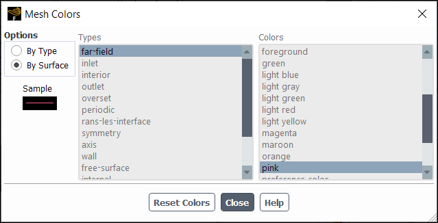
 ), then you can control the colors via the Mesh Colors Dialog Box (the available colors vary depending on
the selected palette and will look like Figure 40.7: The Mesh Colors Dialog Box (Classic Color Scheme) or Figure 40.8: The Mesh Colors Dialog Box (Pastel Color Scheme)) by clicking
in the Mesh Display Dialog Box.
), then you can control the colors via the Mesh Colors Dialog Box (the available colors vary depending on
the selected palette and will look like Figure 40.7: The Mesh Colors Dialog Box (Classic Color Scheme) or Figure 40.8: The Mesh Colors Dialog Box (Pastel Color Scheme)) by clicking
in the Mesh Display Dialog Box.If you are displaying the mesh using the persistent version of the Mesh Display dialog box accessed from the Outline View tree or Results ribbon tab, there are three approaches you can use for controlling the mesh colors—By Type, By Surface, Uniform.
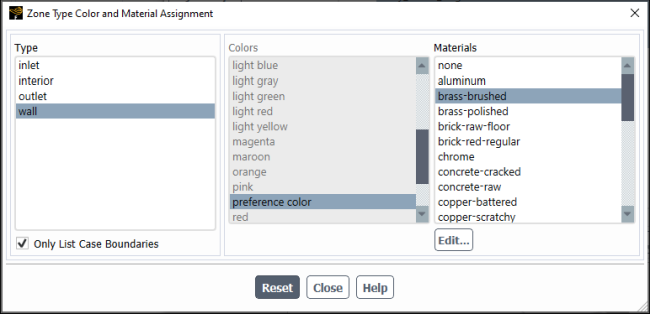
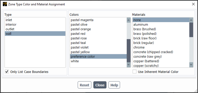
If you are displaying the mesh using the persistent version of the Mesh Display dialog box accessed from the Outline View tree or Results ribbon tab, then you can control the colors via the Zone Type Color and Material Assignment Dialog Box (the available colors vary depending on the selected palette and will look like Figure 40.9: The Zone Type Color and Material Assignment Dialog Box (Classic Color Scheme) or Figure 40.10: Zone Type Color and Material Assignment Dialog Box (Pastel Color Scheme)) by clicking in the Mesh Display Dialog Box.
By Type—Coloring By Type is selected by default in the Mesh Display dialog box. Opening the Zone Type Color and Material Assignment dialog box (by clicking when By Type is selected) lets you assign colors based on zone type. To change the color used to draw the mesh for a particular zone type, select the zone type in the Types list and then select the new color in the Colors list. You will see the effect of your change when you next display the mesh. Note that the surface type in the Types list applies to all surface meshes (that is, meshes that are drawn for surfaces created using the dialog boxes opened from the button in the Surface group box of the Domain ribbon tab) except zone surfaces.
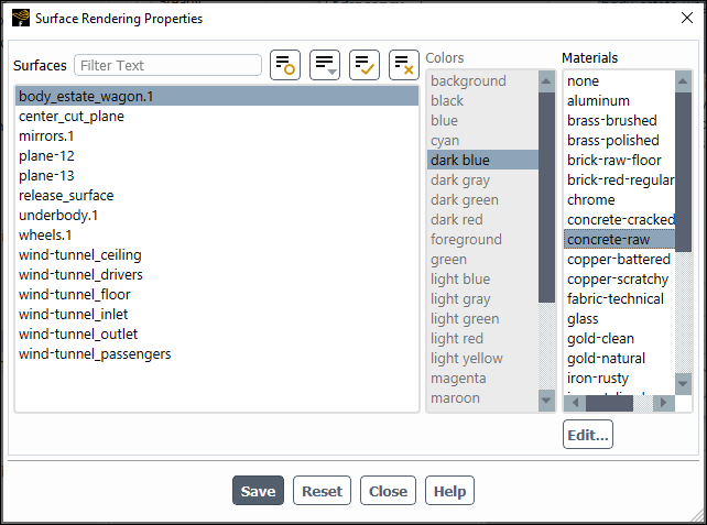
By Surface—Initially, each surface is assigned a random color based on its ID. However, clicking when By Surface is selected opens the Surface Rendering Properties dialog box. Here you can specify a color and/or material for each surface. These settings are preserved, so any subsequent mesh object that you display with By Surface selected will show the same colors/materials that you specify in the Surface Rendering Properties dialog box.
Note: While color and material assignments are local to the selected surfaces when you click , the Use Inherent Material Color option is not. That is, if you change it for one surface, it is changed for all surface color/material assignments.
Uniform—All the selected surfaces are colored according to the specified color and/or material selected in the Faces and Material drop-down lists in the Coloring group box.
You can set colors individually for the meshes displayed on each surface, by selecting the surface(s) in the graphics window, right-clicking and selecting Color by > Color > <color name> from the context menu. Once you have assigned the desired colors, you can right-click and select Save as Scene to create a Scene graphics object containing separate mesh objects for each color you specify.
If you prefer to use the colors Ansys Fluent assigns by zone ID, then you can display the mesh using the By Surface coloring option.
Note: By default, walls are colored by preference color, which indicates that the color of the walls will change based on the Graphics Color Theme specified in Preferences (available from the File ribbon tab). For example, if you change the color theme from Gray Gradient to Black, the wall color will automatically change from black to white to maintain visibility (when preference color is selected for walls).
Randomizing the Mesh Colors
You can use Ctrl+Shift+O to randomize the mesh colors. Ensure the graphics window is in focus by clicking in it before using the hotkey combination (otherwise it won't work).
There are a couple of limitations associated with the color randomization:
Randomizing the colors won't work if the Coloring for the displayed mesh object is set to By Type in the Mesh Display dialog box. It only works for By Surface coloring.
The wall color will not be randomized if the coloring option is set to Color by Type in the Mesh Colors dialog box (in this case, the wall color is taken from Preferences). Note that the colors of all other surface types will still be randomized.
The following sections cover additional details on aspects of realistic material rendering:
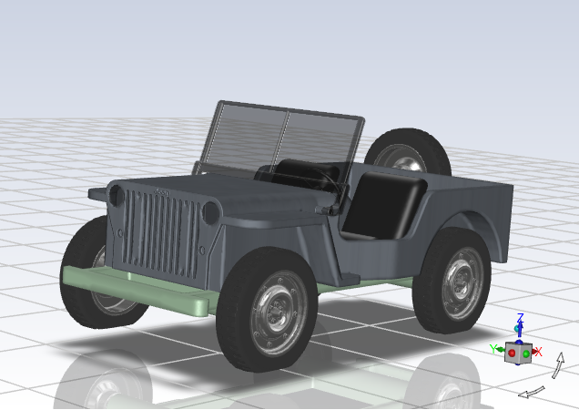
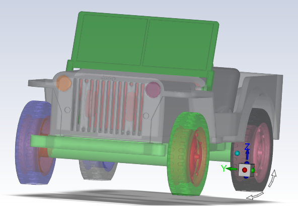
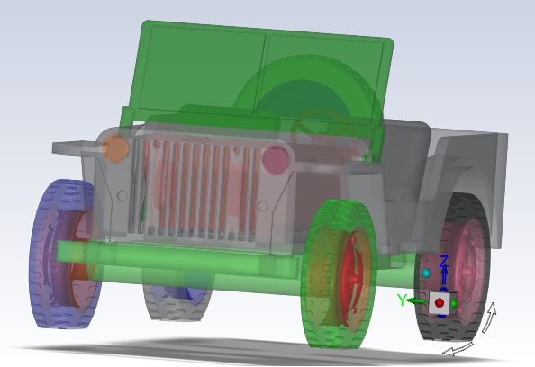
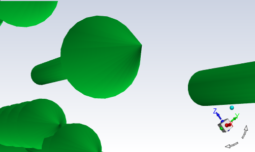
You can assign materials to mesh objects for realistic rendering, as shown in Figure 40.13: Jeep with Multiple Materials Assigned.
You can assign realistic materials to a mesh object as follows:
Using the Mesh Display dialog box.
There are three approaches for coloring surfaces with realistic materials: using the By Type option, using the By Surface option, or using the Uniform option, discussed in By Surface Mesh Coloring and Uniform Mesh Coloring, respectively.
By Surface Mesh Coloring
Coloring By Surface allows you to set a color and/or material for all surfaces at once. Future mesh displays using the By Surface option will be colored using the assignments made in the Surface Rendering Properties dialog box.
Open the Mesh Display dialog box to display a persistent mesh object (this version of the dialog box contains a Mesh Name field and is saved with the case file).
 Results → Graphics → Mesh
→ New...
Results → Graphics → Mesh
→ New...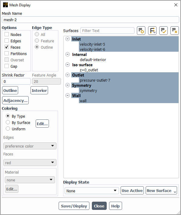
Ensure Faces is enabled in the Options group box.
Select By Surface in the Coloring dialog box.
Click to open the Figure 40.14: Surface Rendering Properties Dialog Box.
Set the desired colors or materials for the surfaces you plan to visualize and click to confirm the assignments. Click when you are done assigning colors and materials to surfaces.
Click .
By Type Mesh Coloring
Coloring By Type allows you to set a color or material for each type of surface (walls, inlets, outlets, and do on). Future mesh displays using the By Type option will be colored using the assignments made in the Zone Type Color and Material Assignments dialog box.
Open the Mesh Display dialog box to display a persistent mesh object (this version of the dialog box contains a Mesh Name field and is saved with the case file).
Results → Graphics → Mesh
→ New...Ensure Faces is enabled in the Options group box.
Select By Type in the Coloring dialog box.
Click to open the Figure 40.15: Zone Type Color and Material Assignment Dialog Box.
Set the desired colors or materials for the surface types you plan to visualize and click to confirm the assignments. Click when you are done assigning colors and materials to surface types.
Click .
Uniform Mesh Coloring
Unlike coloring By Surface, color and material assignments made using this method are only applied for this mesh object and they will not affect any other displays, except scene objects containing this mesh object.
Note: Using Uniform mesh coloring, you can only assign a color or material. If you want to change the color of a material, such as spraypaint, you must create a new material with the color you want. See Creating Custom Realistic Materials for additional information.
Open the Mesh Display dialog box to display a persistent mesh object (this version of the dialog box contains a Mesh Name field and is saved with the case file).
Results → Graphics → Mesh
→ New...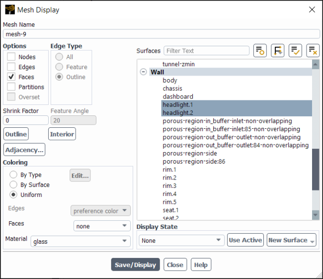
Ensure Faces is enabled in the Options group box.
Select Uniform in the Coloring dialog box.
Select the desired realistic material from the Material drop-down list.
Select the surfaces you want colored with this material in the Surfaces list.
Click .
Using right-mouse-button clicks within the graphics window.
(Assuming the mesh is not already displayed) Right-click in the graphics window and select Display>Mesh....
Ensure Faces is enabled under Options.
Select the mesh surfaces you want displayed in the Surfaces list. click and close the Mesh Display dialog box.
Select the surface(s) you want colored with a realistic material in the graphics window (left-mouse-button-click + Ctrl to select multiple).
Right-click within the graphics window and select Color by>Material>material name.
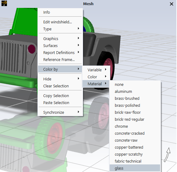
The available materials include:
aluminum
brass-brushed
brass-polished
brick-raw-floor
brick-red-regular
chrome
concrete-cracked
concrete-raw
copper-battered
copper-scratchy
fabric-technical
glass
glass-diamond
gold-clean
gold-natural
iron-rusty
iron-stylized
oil
paint
plastic
rubber
silver-mirror-polished
spray-paint
titanium-brushed
titanium-linear-brushed
water
wood-beech
wood-beech-natural
wood-cedar
Note: You may observe that some of the realistic materials have the same texture, such as brass-brushed and brass-polished. These materials have different bump maps that control the differences in their appearance.
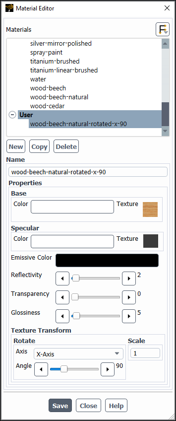
You can use the Material Editor dialog box to create custom materials for realistic rendering.
To create a custom material:
Open the Material Editor dialog box (Figure 40.16: Material Editor Dialog Box) by clicking Material Editor... in the View ribbon tab (Graphics group box).
View
→ Graphics
→ Material Editor...Select the material whose texture most closely matches that of the material you want to create and click . If you do not want to copy an existing material, you can click .
Enter a Name for the new material.
Set the desired material properties.
Select a Base Color by clicking in the colored square to open the Select Color dialog box. Pick your color and click . The base color specifies the primary color of the material.
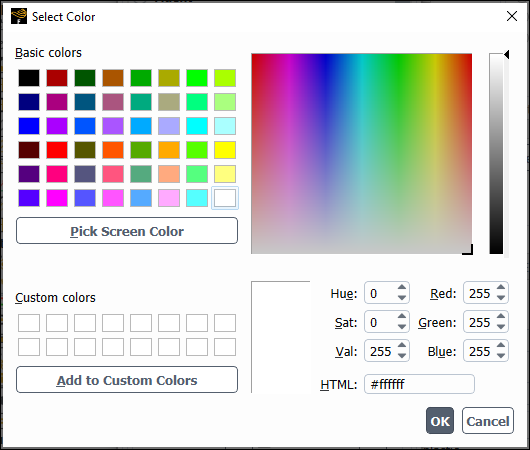
Select a Specular Color by clicking in the colored square to open the Select Color dialog box. Pick your color and click . The specular color specifies the highlight color seen due to lighting effects.
Select a Emissive Color by clicking in the colored square to open the Select Color dialog box. Pick your color and click . The emissive color specifies the color emitted from the material.
Use the slider to set the Reflectivity. Reflectivity specifies how reflective the material appears.
Use the slider to set the Transparency. Transparency specifies how opaque or clear the material appears.
Use the slider to set the Glossiness. Glossiness specifies how glossy the material appears.
Use the Axis drop-down and the Angle slider to rotate the texture by degrees. The Axis drop-down controls which axis the texture is rotated about.
Use the Scale input field to set the desired scaling of the texture. Valid inputs are 0.0004 to 4, with a larger number increasing the size of the texture.
Click to create the new material.
Once a new material is created, it is available for selection in the relevant dialog boxes (Surface Rendering Properties Dialog Box, Zone Type Color and Material Assignment Dialog Box, and Mesh Display Dialog Box). Refer to Realistic Rendering of Materials for guidance on how to use these dialog boxes to achieve your rendering goals.
Note: If you delete a custom material that is being used to color a surface of a currently-displayed graphics object, that surface will become black. Re-display the graphics object to have the black surfaces re-rendered with the default color.
The following limitations exist for the rendering of realistic materials in Fluent:
It is only supported for modern graphics drivers: OpenGL2 (Windows, Linux), DX11 (Windows).
It is not supported for Ansys Fluent in 2D.
It is not supported for the Fluent Remote Visualization Client.
It is not supported from the global mesh display dialog box (accessed by clicking
).Realistic rendering on large cases may reduce graphics performance.
Boundary markers are not compatible with realistic rendering.
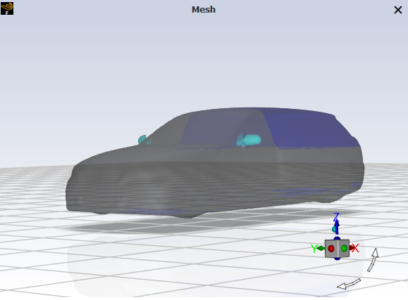
There are multiple ways that you can make the mesh display transparent, as shown in Figure 40.17: Transparent Mesh Display.
Transparency slider in the Figure 40.18: Global Mesh Display Dialog Box.
The global version of the Mesh Display dialog box can by accessed by:
Clicking the mesh display toolbar button (
)Clicking Display... in the General task page (Mesh group box)
 Setup →
  General
→ Mesh
→ Display...
General
→ Mesh
→ Display...Clicking Display... in the Domain ribbon tab (Mesh group box)
Domain
→ Mesh
→ Display...
Clicking the transparency toolbar button (
 ).
). Creating a scene containing a mesh graphics object (Displaying a Scene)
Important: By default, you can only see through 2 layers of displayed transparent surfaces before the remaining transparent surfaces are not rendered. The next surface shown is the next non-transparent (opaque) surface. Refer to Figure 40.19: Mesh Display with Transparency: 2 Layers and Figure 40.20: Mesh Display with Transparency: 3 Layers to see an example.
You can control the transparency technique and the number of transparent layers using the Transparency Algorithm for Modern Graphics Drivers and Depth Peeling Layers for Transparency settings under Transparency in the Graphics branch of Preferences (File>Preferences...).
The options mentioned in the procedure in the previous section include modifying the mesh colors, adding the outline of important features to an outline display, drawing partition boundaries, and shrinking the faces and/or cells in the display.
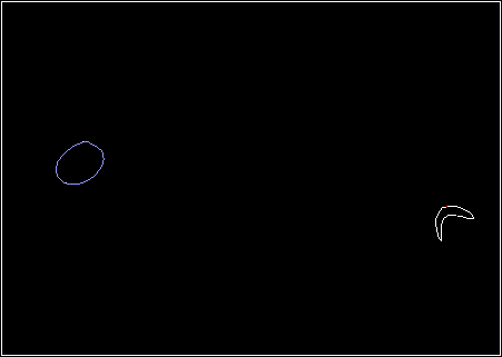
For closed 3D geometries such as cylinders, the standard outline display often will not show enough detail to accurately depict the shape. This is because for each boundary, only those edges on the “outside” of the geometry (that is, those that are used by only one face on the boundary) are drawn. In Figure 40.21: Standard Outline of Complex Duct, which shows the outline display for a complicated duct geometry, only the inlet and outlet are visible.
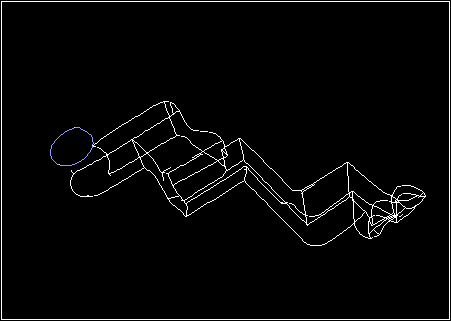
You can capture additional features using the Feature option in the Mesh Display Dialog Box. (See Figure 40.22: Feature Outline of Complex Duct.) Enable Feature under Edge Type, and then set the Feature Angle. With the default Feature Angle of 20, if the difference between the normal directions of two adjacent faces is more than 20°, the edge between those faces will be drawn. Decreasing the Feature Angle will result in more edge lines (that is, more detail) being added to the outline display. The appropriate angle for your geometry will depend on its curvature and complexity. You can modify the Feature Angle until you find the value that yields the best outline display.
If you have partitioned your mesh for parallel processing, you can add the display of partition boundaries to the mesh display by turning on the Partitions option in the Mesh Display Dialog Box.
To distinguish individual faces or cells in the display, enlarge the space between adjacent faces or cells by increasing the Shrink Factor in the Mesh Display Dialog Box. The default value of zero produces a display in which the edges of adjacent faces or cells overlap. A value of 1 creates the opposite extreme: each face or cell is represented by a point and there is considerable space between each one. A small value such as 0.01 may be large enough to enable you to distinguish one face or cell from its neighbor. Displays with different Shrink Factor values are shown in Figure 40.23: Mesh Display with Shrink Factor = 0 and Figure 40.24: Mesh Display with Shrink Factor = 0.01. Click to see the effect of the change in Shrink Factor.
You can create named mesh plot definitions and save them for later use. See Creating and Using Contour Plot Definitions for additional information on graphics object definitions.
The steps for creating and using mesh plot definitions are similar to the steps for Generating Mesh or Outline Plots, with the addition of a field for naming the mesh plot definition.
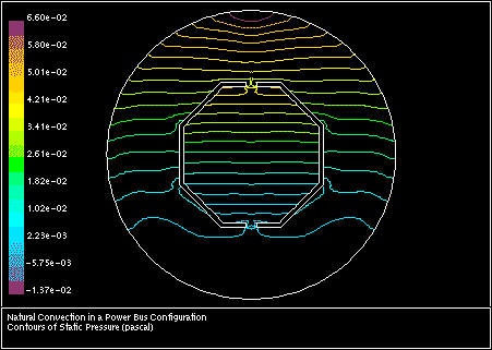
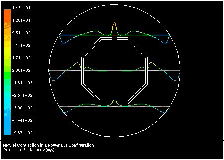
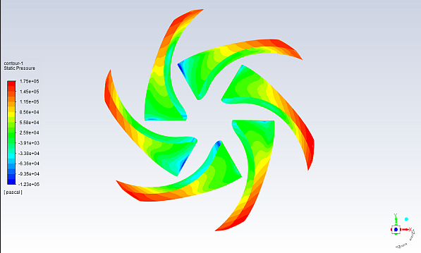
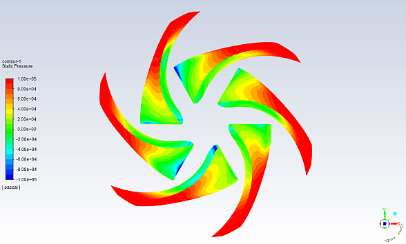
Ansys Fluent enables you to plot contour lines or profiles superimposed on the physical domain. Contour lines are lines of constant magnitude for a selected variable (isotherms, isobars, and so on). A profile plot draws these contours projected off the surface along a reference vector by an amount proportional to the value of the plotted variable at each point on the surface. Sample plots are shown in Figure 40.25: Contours of Static Pressure and Figure 40.26: Profile Plot of y Velocity.
For information about displaying contours or profiles on a surface that sweeps through the domain, see Displaying Results on a Sweep Surface.
Contours are only displayed in regions where the variable is defined and relevant, which primarily applies to fluid-structure interaction cases (FSI). For example, deflection is not displayed in fluid cell zones, as this variable has no meaning in a fluid. This only applies to predefined fields—expressions and custom field functions will display values in all cell zones.
Note: By default, the surfaces of contour plots do not have any reflective properties. However, you can make the surfaces appear more reflective and shiny by increasing the Surface specularity for Contours field under the Appearance branch in Preferences.
Once there is data associated with your case, you can quickly visualize the results with a contour plot in the graphics window.
To create a plot directly in the graphics window:
Select the desired surfaces for visualizing the results using Ctrl + left-click.
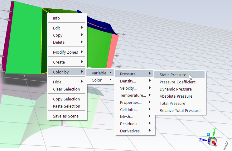
Right-click in the graphics window and select Color by>Variable | Color> desired color or variable. See Figure 40.27: Coloring Surfaces by Static Pressure for an example.
You can color different surfaces by different colors or variables and they will be added to the same graphics window, which is similar to creating a scene (Displaying a Scene).
You can choose to save the current graphics window display for later use by select the Save as Scene right-click menu option. This creates graphics objects for the items displayed in the graphics window (for example, mesh and contours) and adds them to a scene graphics object. Refer to Basic Graphics Generation and Generating a Scene for additional information on creating and manipulating graphics objects.
Note that saving the current graphics window as a scene also saves the display state, which preserves the orientation, graphics effects, and other graphics settings. Refer to Controlling the Display State and Modifying the View for additional information.
You can plot contours or profiles using the Contours Dialog Box (Figure 40.28: The Contours Dialog Box).
Important: If you plan to plot profiles, you must enable the Expose non-persistent graphics option in the Graphics branch of Preferences (accessed by File>Preferences...), because profiles can only be displayed using the non-persistent contours object, accessed via the Edit... option.
![]() Results → Graphics →
Contours
Results → Graphics →
Contours ![]() New...
New...
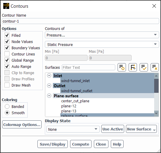
The basic steps for generating a contour or profile plot are as follows:
Select the variable or function to be contoured or profiled in the Contours of drop-down list. First select the desired category in the upper list; you may then select a related quantity in the lower list. (See Field Function Definitions for an explanation of the variables in the list.)
Choose the surface or surfaces on which to draw the contours or profiles in the Surfaces list. For 2D cases, if no surface is selected, contouring or profiling is done on the entire domain. For 3D cases, you must always select at least one surface.
If you want to select several surfaces of the same type, click
and select Surface Type under
Group By, which organizes the surfaces in a
tree view that is grouped by surface type.Another shortcut is to use the Filter Text entry box to filter the Surfaces list to show only the surfaces that match the pattern you enter. For additional information on using the Filter Text entry box, see Filter Text Entry Boxes.
Specify the number of contours or profiles in the Levels field. The maximum number of levels allowed is 100.
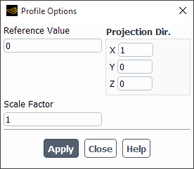
If you are generating a profile plot, enable the Draw Profiles option. In the resulting Profile Options Dialog Box (Figure 40.29: The Profile Options Dialog Box) you will define the profiles.
Note: Draw Profiles is only available for the non-persistent/"global" version of the Contours dialog box that does not have a Name field. This version of the dialog box must first made available by enabling the Expose non-persistent graphics option in the Graphics branch of Preferences (accessed by File>Preferences...). It is then opened by:
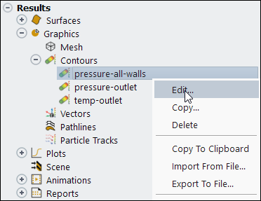
Right-clicking Contours in the Outline View tree and selecting Edit... (located under the Results branch).
Clicking Contours and selecting Edit... under Graphics in the Results ribbon tab.
Set the “zero height” reference value for the profile (Reference Value) and the length scale factor for projection (Scale Factor). Any point on the profile with a value equal to the Reference Value will be plotted exactly on the defining surface. Values greater than the Reference Value will be projected ahead of the surface (in the direction of Projection Dir.) and scaled by Scale Factor), and values less than the Reference Value will be projected behind the surface and scaled.
These parameters can be used to create fuller profiles when you need to display the variation in a variable that is small compared to the absolute value of the variable. Consider, for example, the display of temperature profiles when the temperature range in the domain is from 300 K to 310 K. The 10 K range in the temperature will be hard to detect when profiles are drawn using the default scaling (which will be based on the absolute magnitude of 310 K). To create a fuller profile, you can set the Reference Value to 300 and the profile Scaling Factor to 5 (for example) to magnify the display of the remaining 10 K range. In subsequent display of the profiles, the reference value of 300 will be effectively subtracted from the data before display so that the temperatures of 300 K will not be offset from the baselines. The profiles will then reflect only the variation of temperature from 300 K.
Set the direction in which profiles are projected (Projection Dir.). In 2D, for example, a contour plot of pressure on the entire domain can be projected in the
 direction to form a carpet
plot, or a contour plot of
direction to form a carpet
plot, or a contour plot of  velocity on a sequence of
  -coordinate slice lines can be
projected in the
-coordinate slice lines can be
projected in the  direction to form a series of velocity profiles
(as shown in Figure 40.26: Profile Plot of y Velocity).
direction to form a series of velocity profiles
(as shown in Figure 40.26: Profile Plot of y Velocity).Click and close the Profile Options Dialog Box.
Set any of the contour and profile plot options described below.
Click to draw the specified contours or profiles in the active graphics window.
(Optional) Associate a display state with this contour plot for a consistent appearance each time the contour plot is redisplayed.
Set the display state. There are two approaches:
Setup the graphics window with your preferred model orientation, zoom level, graphics effects, ruler, and so on, and click to create a display state with these properties.
Select a display state from the Display State drop-down list (if you already created a display state that you would like to reuse for other graphics objects).
Click to link the selected display state with this contour plot.
Refer to Controlling the Display State and Modifying the View for additional information.
The resulting display will include the specified number of contours or profiles of the selected variable, with the magnitude on each one determined by equally incrementing between the values shown in the Min and Max fields.
The options mentioned in the procedure above include drawing color-filled contours/profiles (instead of the default line contours/profiles), specifying a range of values to be contoured or profiled, including portions of the mesh in the contour or profile display, choosing node or cell values for display, and storing the contour or profile plot settings.
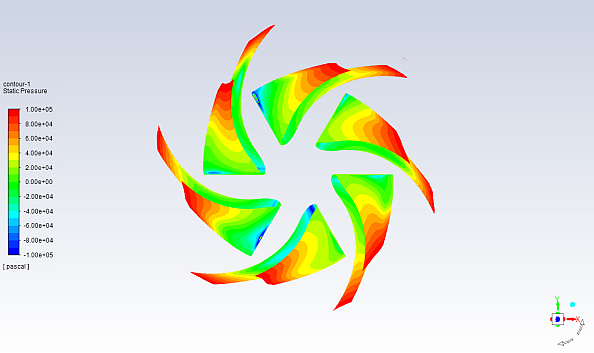
Color-filled contour or profile plots show a contour or profile display containing a continuous color display (see Figure 40.30: Filled Contours of Static Pressure), instead of just drawing lines representing specific values. Note that a color-filled profile display is often referred to as a “carpet plot”. To generate a filled contour or profile plot, enable the Filled option in the Contours Dialog Box during step 5 in the previous section.
To display smoothly shaded filled contours, ensure the lighting interpolation method is not set to Flat in the Display Options Dialog Box or the Lights Dialog Box. You will not get smooth shading of filled contours if the Clip to Range option is turned on. Smooth shading of filled profiles is not available.
Note: The Draw Profile option settings are not saved with the contour plot definition. Once the dialog box is closed these options will revert to being disabled.
By default, the minimum and maximum values contoured or profiled are set based on the range of values in the entire domain. This means that the color scale will start at the smallest value in the domain (shown in the Min field) and end at the largest value (shown in the Max field). If you are plotting contours or profiles on a subset of the domain (that is, on a surface), your plot may cover only the midrange of the color scale. For example, if blue corresponds to 0 and red corresponds to 10, and the values on your surface range only from 4 to 6, your plot will contain mostly green contours or profiles, since green is the color at the middle of the default color scale.
To focus in on a smaller range of values, so that blue corresponds to 4 and red to 6, manually reset the range to be displayed. You can also use the minimum and maximum values on the selected surfaces—rather than in the entire domain—to determine the range. Another reason to manually set the range is if you are interested only in certain values. For example, if you want to determine the region where pressure exceeds a certain value, you can increase the minimum value for display so that the lower pressure values are not displayed.
To manually set the contour/profile range, turn off the Auto Range option in the Contours Dialog Box. The Min and Max fields will become editable, and you can enter the new range of values to be displayed.
To show the default range at any time, click and the Min and Max fields will be updated.
If you are drawing filled contours or profiles you can control whether or not values outside the prescribed Min/ Max range are displayed.
To leave areas in which the value is outside the specified range empty (that is, draw no contours or profiles), enable the Clip to Range option. This is the default setting. If you turn Clip to Range off, values below the Min value will be colored with the lowest color on the color scale, and values above the Max value will be colored with the highest color on the color scale. Figure 40.31: Filled Contours with Clip to Range On and Figure 40.32: Filled Contours with Clip to Range Off show the results of enabling/disabling the Clip to Range option.
To base the minimum and maximum values on the range of values on the selected surfaces, rather than in the entire domain, turn off the Global Range option in the Contours Dialog Box. The Min and Max values will be updated when you next click Compute or .
Note: When Global Range is enabled, Fluent only computes and populates the range when:
You click .
Auto Range is enabled.
If Auto Range is disabled, the range will remain the same until you click , even if you select a new variable for display.
For some problems, especially complex 3D geometries, you may want to include portions of the mesh in your contour or profile plot as spatial reference points. For example, you may want to show the location of an inlet and an outlet along with the contours. This is accomplished by turning on the Draw Mesh option in the Contours Dialog Box. The Mesh Display Dialog Box will appear automatically when you enable the Draw Mesh option, and you can set the mesh display parameters there. When you click in the Contours Dialog Box, the mesh display, as defined in the Mesh Display Dialog Box, will be included in the contour or profile plot.
Note: The Draw Mesh option settings are not saved with the contour plot definition. Once the dialog box is closed these options will revert to being disabled.
To include the mesh with a contour plot that will be persisted with the case file, you can create a mesh plot definition and include both the mesh and contour plots in a scene. See Displaying a Scene for more details.
In Ansys Fluent you can choose to display the computed cell-center values or values that have been interpolated to the nodes. By default, the Node Values option is turned on, and the interpolated values are displayed. For line contours or profiles, node values are always used. To display filled contours or profiles and to display the cell values, turn off the Node Values option. Filled contours/profiles of node values will show a smooth gradation of color, while filled contours/profiles of cell values may show sharp changes in color from one cell to the next.
Enabling Boundary Values in addition to Node Values, displays interpolated boundary face values, when available. If Boundary Values are enabled with Node Values disabled, then the displayed values are boundary face values (not interpolated), if available. Variables that have explicit node values available at boundaries are indicated by "bnv" in Table 42.2: Pressure and Density Categories – Table 42.21: Acoustics Category . Note that when Boundary Values is enabled and velocity contours are selected for postprocessing, Fluent reports the user-specified wall velocity values for wall zones.
The displayed values are derived as follows:
Node Values and Boundary Values enabled means that node values are displayed that are interpolated from boundary face values, as seen in Figure 40.33: Contours of Velocity Magnitude on a Wall + Outlet: Node Values + Boundary Values Enabled.
Figure 40.33: Contours of Velocity Magnitude on a Wall + Outlet: Node Values + Boundary Values Enabled

Node Values disabled and Boundary Values enabled means that boundary face values are displayed, as seen in Figure 40.34: Contours of Velocity Magnitude: Node Values Disabled + Boundary Values Enabled .
Node Values enabled and Boundary Values disabled means that node values are displayed that interpolated from adjacent cell values, as seen in Figure 40.35: Contours of Velocity Magnitude: Node Values Enabled + Boundary Values Disabled.
Node Values disabled and Boundary Values disabled means that adjacent cell values are displayed, as seen in XREF.


For face-only functions (for example, Wall Shear Stress), the cell values that are displayed for boundary zone surfaces will actually be the face values. This is only true in the case of boundary zone surfaces created for postprocessing, where the actual cell values are used for the part of the surface that lies in the interior. These face values are more accurate, as face-only functions are computed on the faces and not on the cells. For more information about cell values, see Cell Values.
If you are plotting contours to show the effect of a porous medium or 2D fan boundary, to depict a shock wave, or to show any other discontinuities or jumps in the plotted variable, you should use cell values; if you use node values in such cases, the discontinuity will be smeared by the node averaging for graphics and will not be shown clearly in the plot.
Important:
If you are comparing contours at boundaries with different postprocessing methods such as reports or XY plots, then you must ensure that the Boundary Values option is enabled in the Contours dialog box to see consistent, comparable results.
Results may differ for coupled walls that are intersecting boundaries. That is, you may see different results on a wall as compared to its wall-shadow depending on whether Node Values are enabled/disabled in this scenario.
For frequently used combinations of contour variables and options, you can store the information needed to generate the contour plot as follows:
In the Contours Dialog Box, specify a Setup number.
Set up the desired information in the Contours Dialog Box.
Click .
The settings for Options, Contours of, Min, Max, and Surfaces will be saved.
You can then change the Setup number to an unused value (that is, an ID for which no information has been saved) and generate a different contour plot.
To generate a plot using the saved setup information:
Change the Setup number back to the value for which you saved contour information.
Click .
You can save up to 10 different setups.
Important: Note that the number of contour Levels, the surfaces selected for display in the Mesh Display Dialog Box (when the Draw Mesh option is activated), and the settings for profiles in the Profile Options Dialog Box (when the Draw Profiles option is activated) will not be saved in the Setup, nor will the Setup be saved in the case file.
You can create named contour plot definitions and save them for later use. This could be useful for demonstration purposes, scene creation, or for postprocessing the results of your simulation when varying the settings between runs (to name a few examples).
The number of contour plot definitions is not limited.
To create a contour plot definition:
![]() Results → Graphics → Contours
Results → Graphics → Contours![]() New...
New...
In the Contours Dialog Box, in the Contour Name text entry box, enter the name for your contour plot definition (or accept the default name
contour-).idImportant: Contour and vector plot definitions must have unique names.
Set contour parameters and options.
The Draw Mesh and Draw Profile option settings are not saved with the contour plot definition. Once the dialog box is closed these options will revert to being disabled.
Click .
The specified contour will be displayed in the active graphics window, and the new contour plot definition with the name you have entered will appear in the tree under Contours.
Once the contour plot definition is created, you can perform the following actions using the right-click menu commands:
Edit the existing contour plot definition.
Copy the contour plot definition.
When creating a copy of the existing contour, you can modify contour settings in the Contours dialog box that will open.
Delete the selected contour plot definition.
Display the contour in the graphics window.
Add the selected contour to the plot in the graphics window.
Note that while Display replaces the current contents of the graphics window, the Add to menu option preserves the current graphics window contents.
Note:
You can move the colormap of contour plot definitions by left-clicking and dragging it to the desired location. The colormap can also be resized by dragging the corners of the box that appears when you hover over the colormap. The colormap location is not saved with the contour plot definition.
For 2D cases, Fluent automatically creates a new surface when you click in the Contours dialog box, if you have not selected any surfaces for display. New surfaces are only created for fluid zones that do not already have a surface defined.
These commands are also available through the text user interface
(display/objects).
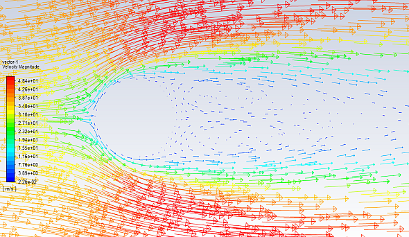
You can draw vectors in the entire domain, or on selected surfaces. By default, one vector is drawn at the center of each cell (or at the center of each facet of a data surface), with the length and color of the arrows representing the velocity magnitude (Figure 40.37: Velocity Vector Plot). The spacing, size, and coloring of the arrows can be modified, along with several other vector plot settings. Velocity vectors are the default, but you can also plot vector quantities other than velocity. Note that cell-center values are always used for vector plots; you cannot plot node-averaged values.
For information about displaying vectors on a surface that sweeps through the domain, see Displaying Results on a Sweep Surface.
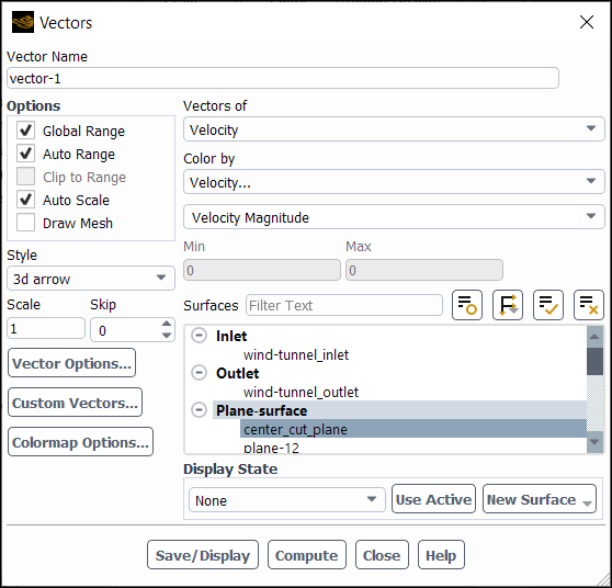
You can plot vectors using the Vectors Dialog Box (Figure 40.38: The Vectors Dialog Box).
![]() Results → Graphics →
Vectors
Results → Graphics →
Vectors ![]() New...
New...
The procedure for generating a vector plot is as follows:
In the Vectors of drop-down list, select the vector quantity to be plotted. By default, only velocity and relative velocity are available, but you can create your own custom vectors as described in Creating and Managing Custom Vectors. Additional vector options are available for adjoint solver results, as described in Field Data.
In the Surfaces list, choose the surface(s) on which you want to display vectors. If you want to display vectors on the entire domain, select none of the surfaces in the list.
If you want to select several surfaces of the same type, click
and select Surface Type under
Group By, which organizes the surfaces in a
tree view that is grouped by surface type.Another shortcut is to use the Filter Text entry box to filter the Surfaces list to show only the surfaces that match the pattern you enter. For additional information on using the Filter Text entry box, see Filter Text Entry Boxes.
Set any of the vector plot options as described in Vector Plot Options.
Click to draw the vectors in the active graphics window.
(Optional) Associate a display state with this vector plot for a consistent appearance each time the vector plot is redisplayed.
Set the display state. There are two approaches:
Setup the graphics window with your preferred model orientation, zoom level, graphics effects, ruler, and so on, and click to create a display state with these properties.
Select a display state from the Display State drop-down list (if you already created a display state that you would like to reuse for other graphics objects).
Click to link the selected display state with this vector plot.
Refer to Controlling the Display State and Modifying the View for additional information.
If you are solving your problem using one or more moving reference frames or moving meshes, you will have the option to display either the absolute vectors or the relative vectors. If you select Velocity (the default) in the Vectors of list, the vectors will be drawn based on the absolute, stationary reference frame. If you select Relative Velocity, the vectors will be drawn based on the reference frame of the Reference Zone in the Reference Values Task Page. See Setting the Reference Zone for details. (If you are modeling a single moving reference frame, you need not specify the Reference Zone; the vectors will be drawn based on the moving reference frame.)
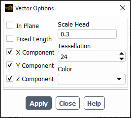
The options mentioned in the procedure above include scaling the vector arrows, skipping the display of some vectors, displaying vectors in the plane of the data surface, displaying fixed-length or fixed-color vectors, displaying directional components of the vectors, specifying a range of values to be displayed, adjusting the tessellation of 3D vectors, coloring the vectors by a different scalar field, including portions of the mesh in the vector display, and changing the style of the arrows or the scale of the arrowheads.
The most common options are set in the Vectors Dialog Box, and others are set in the Vector Options Dialog Box (Figure 40.39: The Vector Options Dialog Box), which you can open by clicking in the Vectors Dialog Box.
By default, vectors are scaled automatically so that the arrows overlap minimally when no vectors are skipped. For instructions on thinning the vector display, see “Thinning” Pathlines. With the Auto Scale option, you can modify the Scale factor (which is set to 1 by default) to increase or decrease the vector scale from the default “auto scale”. The main advantage of autoscaling is that the vector display with a scale factor of 1 will always be appropriate, regardless of the size of the domain, giving you a better starting point for fine-tuning the vector scale.
If you turn off the Auto Scale option, the vectors will be drawn at their actual sizes scaled by the scale factor (Scale, which is set to 1 by default). The “actual” size of a vector is the magnitude of the vector variable (velocity, by default) at the point where it is drawn. A vector drawn at a point where the velocity magnitude is 100 m/s is drawn 100 m long, whether the domain is 0.1 m or 1000 m. You can modify the vector scale by changing the value of Scale in the Vectors Dialog Box until the size of the vectors (that is, the actual size multiplied by Scale) is satisfactory.
Note: Vectors may appear larger than they did for the same values in previous releases. You can control the size of vectors using the Scale setting in the Vectors dialog box.
If your vector display is difficult to understand because there are too
many arrows displayed, you can “thin out” the vectors by
changing the Skip value in the Vectors Dialog Box. By default, Skip is set
to 0, indicating that a vector will be drawn for each cell in the domain or
for each face on the selected surface (for example,  vectors). If you increase Skip to 1,
every other vector will be displayed, yielding
vectors). If you increase Skip to 1,
every other vector will be displayed, yielding  vectors. If you increase Skip to 2,
every third vector will be displayed, yielding
vectors. If you increase Skip to 2,
every third vector will be displayed, yielding  vectors, and so on. The order of faces on the selected
surface (or cells in the domain) will determine which vectors are skipped or
drawn; therefore adaption will change the appearance of the vector display
when a nonzero Skip value is used.
vectors, and so on. The order of faces on the selected
surface (or cells in the domain) will determine which vectors are skipped or
drawn; therefore adaption will change the appearance of the vector display
when a nonzero Skip value is used.
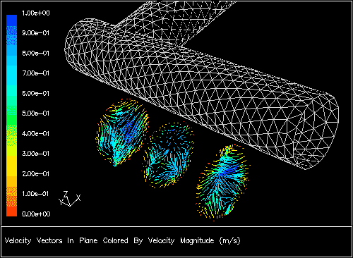
For some problems, you may be interested in visualizing velocity (or other vector) components that are normal to the flow. These “secondary flow” components are usually much smaller than the components in the flow direction and are difficult to see when the flow direction components are also visible. To easily view the normal flow components, you can enable the In Plane option in the Vector Options Dialog Box. When this option is on, Ansys Fluent will display only the vector components in the plane of the surface selected for display. If the selected surface is a cross-section of the flow domain, you will be displaying the components normal to the flow.
Figure 40.40: Velocity Vectors Generated Using the In Plane Option shows velocity vectors generated using the In Plane option. Note that these vectors have been translated outside the domain, as described in Transforming Geometric Objects in a Scene, so that they can be seen more easily.
By default, the length of a vector is proportional to its velocity magnitude. If you want all of the vectors to be displayed with the same length, you can enable the Fixed Length option in the Vector Options Dialog Box. To modify the vector length, adjust the value of the Scale factor in the Vectors Dialog Box.
All Cartesian components of the vectors are drawn by default,
so that the arrow points along the resultant vector in physical space.
However, sometimes one of the components, say, the  component, is relatively
large. In such cases, you may want to suppress the
component, is relatively
large. In such cases, you may want to suppress the  component and scale up the
vectors, in order to visualize the smaller
component and scale up the
vectors, in order to visualize the smaller  and
and  components. To suppress one or
more of the vector components, turn off the appropriate button(s)
(X, Y, or Z Component) in the Vector Options Dialog Box.
components. To suppress one or
more of the vector components, turn off the appropriate button(s)
(X, Y, or Z Component) in the Vector Options Dialog Box.
By default, the minimum and maximum vectors included in the vector display are set based on the range of vector-variable (velocity, by default) magnitudes in the entire domain. If you want to focus in on a smaller range of values, you can restrict the range to be displayed. The color scale for the vector display will change to reflect the new range of values. (You can also use the minimum and maximum values on the selected surfaces—rather than on the entire domain—to determine the range, or change the scalar field by which the vectors are colored from velocity magnitude to any other scalar, as described below.)
To manually set the range of velocity magnitudes (or the range of whatever scalar field is selected in the Color by drop-down list), turn off the Auto Range option in the Vectors Dialog Box. The Min and Max fields will become editable, and you can enter the new range of values to be displayed. For example, if you want to display velocity vectors only in regions where the velocity magnitude exceeds 150 m/s but is less than 300 m/s, you will change the value of Min to 150 and the value of Max to 300. Similarly, if you are coloring the vectors by static pressure, you can choose to display velocity vectors only in regions where the pressure is within a specified range. To show the default range at any time, click and the Min and Max fields will be updated.
When you restrict the range of vectors displayed, you can also control whether or not values outside the prescribed Min/ Max range are displayed. To leave areas in which the value is outside the specified range empty (that is, draw no vectors), enable the Clip to Range option. This is the default setting. If you turn Clip to Range off, values below the Min value will be colored with the lowest color on the color scale, and values above the Max value will be colored with the highest color on the color scale. This feature is the same as the one available for displaying filled contours (see Figure 40.31: Filled Contours with Clip to Range On and Figure 40.32: Filled Contours with Clip to Range Off).
You can also choose to base the minimum and maximum values on the range of values on the selected surfaces, rather than the entire domain. To do this, turn off the Global Range option in the Vectors Dialog Box. The Min and Max values will be updated when you next click or .
If you want to color the vectors by a scalar field other than velocity magnitude (the default), you can select a different variable or function in the Color by drop-down list. Select the desired category in the upper list, and then choose one of the related quantities from the lower list. If you choose static pressure, for example, the length of the vectors will still correspond to the velocity magnitude, but the color of the vectors will correspond to the value of pressure at each point where a vector is drawn.
You can adjust the tessellation of the 3d arrow and
3d arrowhead vector plot Styles.
This control has a valid range of 0-74.
Tessellation is accessed by clicking Vector Options... in the Vectors dialog box. Tessellation affects how round the edges of the cylinder and arrowhead appear. Lower values appear less round, which comes with some performance benefit in rendering the vector plot.
If you want all of the vectors to be the same color, you can select the color to be used in the Color drop-down list in the Vector Options Dialog Box. If no color is selected (that is, if you choose the empty space at the top of the drop-down list—the default selection), the vector color will be determined by the Color by field specified in the Vectors Dialog Box. Single color vectors are useful in displays that overlay contours and vectors.
For some problems, especially complex 3D geometries, you may want to include portions of the mesh in your vector plot as spatial reference points. For example, you may want to show the location of an inlet and an outlet along with the vectors. This is accomplished by turning on the Draw Mesh option in the Vectors Dialog Box. The Mesh Display Dialog Box will appear automatically when you enable the Draw Mesh option, and you can set the mesh display parameters there. When you click in the Vectors Dialog Box, the mesh display, as defined in the Mesh Display Dialog Box, will be included in the vector plot.
Note: The Draw Mesh option settings are not saved with the vector plot definition. Once the dialog box is closed these settings will revert to being disabled.
To include the mesh with a vector plot that will be persisted with the case file, you can create a mesh plot definition and include both the mesh and vector plots in a scene. See Displaying a Scene for more details.
There are seven different vector arrow styles available. Choose 3d arrow, 3d arrowhead, cone, filled-arrow, arrow, harpoon, or headless in the Style drop-down list in the Vectors Dialog Box.
If you choose a vector arrow style that includes heads, you can control the size of the arrowhead by modifying the Scale Head value in the Vector Options Dialog Box.
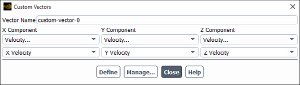
In addition to the velocity vector quantity provided by Ansys Fluent, you can also define your own custom vectors to be plotted. This capability is available with the Custom Vectors Dialog Box.
Any custom vectors that you define will be saved in the case file the next time that you save it. You can also save your custom vectors to a separate file, so that they can be used with a different case file.
To create your own custom vector, you will use the Custom Vectors Dialog Box (Figure 40.43: The Custom Vectors Dialog Box). This dialog box enables you to define custom vectors based on existing quantities. Any vectors that you define will be added to the Vectors of list in the Vectors Dialog Box.
To open the Custom Vectors Dialog Box, click in the Vectors Dialog Box.
The steps for creating a custom vector are as follows:
Specify the name of the custom vector in the Vector Name field.
Important: Do not specify a name that is already used for a standard vector (for example,
velocityorrelative-velocity).Select the variable or function for the x component of the vector in the X Component drop-down list. First select the desired category in the upper list; you may then select a related quantity in the lower list. For an explanation of the variables in the list, see Field Function Definitions.
Repeat the step above to select the variable or function for the
 component (and, in 3D, the
  component) of the custom vector.
Important: You can use the Custom Vectors option to plot vectors in solid cell zones. The scalars that are selected in the x, y (and, in 3D, the z) components, and that are valid in solid regions, will have vector plots displayed in the solid cell zones. Note that if a vector has no valid components in the solid region, then that vector will not be plotted in the solid region. However, if at least one component of the vector is valid in the solid region, then only that component of the vector will be plotted.
Click .
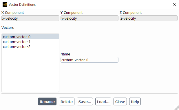
Once you have defined your vectors, you can manipulate them using the Vector Definitions Dialog Box (Figure 40.44: The Vector Definitions Dialog Box). You can display a vector definition to be sure that it is correct, delete the vector if you decide that it is incorrect and must be redefined, or give the vector a new name. You can also save custom vectors to a file or read them from a file. The custom vector file enables you to transfer custom vectors between case files.
To open the Vector Definitions Dialog Box, click in the Custom Vectors Dialog Box.
The following actions can be performed in the Vector Definitions Dialog Box:
To check the definition of a vector, select it in the Vectors list. Its definition will be displayed in the X Component, Y Component, and Z Component fields at the top of the dialog box. This display is for informational purposes only; you cannot edit it. If you want to change a vector definition, you must delete the vector and define it again in the Custom Vectors Dialog Box.
To delete a vector, select it in the Vectors list and click .
To rename a vector, select it in the Vectors list, enter a new name in the Name field, and click .
Important: Do not specify a name that is already used for a standard vector (for example,
velocityorrelative-velocity).To save all the vectors in the Vectors list to a file, click and specify the file name in The Select File Dialog Box.
To read custom vectors from a file that you saved as described above, click and specify the file name in The Select File Dialog Box. (Custom vectors are valid Scheme functions, and can also be loaded with the File/Read/Scheme... ribbon tab item, as described in Reading Scheme Source Files.)
You can create named vector plot definitions and save them for later use. See Creating and Using Contour Plot Definitions for additional information on plot definitions.
The steps for creating and using vector plot definitions are similar to the steps for Generating Vector Plots, with the addition of a field for naming the vector plot definition.
Note: You can move the colormap of a vector plot definition by left-clicking and dragging it to the desired location. The colormap can also be resized by dragging the corners of the box that appears when you hover over the colormap. The colormap location is not saved with the vector plot definition.
Pathlines are used to visualize the flow of massless particles in the problem domain. The particles are released from one or more surfaces that you have created by clicking in the Surface group box of the Domain ribbon tab (see Creating Surfaces and Cell Registers for Displaying and Reporting Data). A line or rake surface (see Line and Rake Surfaces) is most commonly used. Figure 40.45: Pathline Plot shows a sample plot of pathlines.
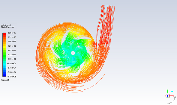
Note that the display of discrete-phase particle trajectories is discussed in Displaying of Trajectories.
You can plot pathlines using the Pathlines Dialog Box (Figure 40.46: The Pathlines Dialog Box).
![]() Results → Graphics →
Pathlines
Results → Graphics →
Pathlines ![]() New...
New...
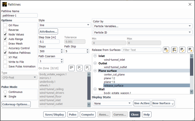
The basic steps for generating pathlines are as follows:
Select the surface(s) from which to release the particles in the Release From Surfaces list.
(Eulerian Multiphase model only) From the Track in Phase drop-down list, select the phase in which pathlines will be tracked. If you want to track pathlines in the mixture of all phases, select all-phase. By default, particles are tracked in the primary phase.
Set the step size and the maximum number of steps. The Step Size sets the length interval used for computing the next position of a particle. Note that particle positions are always computed when particles enter/leave a cell; even if you specify a very large step size, the particle positions at the entry/exit of each cell will still be computed and displayed. The value of Steps sets the maximum number of steps a particle can advance. A particle will stop when it has traveled this number of steps or when it leaves the domain. One simple rule of thumb to follow when setting these two parameters is that if you want the particles to advance through a domain of length
 , the Step Size times the number of Steps should be approximately
equal to
, the Step Size times the number of Steps should be approximately
equal to  .
.Set any of the pathline plot options described in Options for Pathline Plots.
Click to draw the pathlines, or click to animate the particle positions. The button will become the button during the animation, and you must click to stop the pulsing.
Note: Enable Save Pulse Animation to save a video or picture files of the pulse animation. When this option is enabled, an additional Write/Record Format drop-down list appears that controls what type of file is written when you click Save/Write....
A Continuous pulse video file will be 5 seconds long, while a Single pulse video will be one full cycle.
(Optional) Associate a display state with this pathline plot for a consistent appearance each time the pathline plot is redisplayed.
Set the display state. There are two approaches:
Setup the graphics window with your preferred model orientation, zoom level, graphics effects, ruler, and so on, and click to create a display state with these properties.
Select a display state from the Display State drop-down list (if you already created a display state that you would like to reuse for other graphics objects).
Click to link the selected display state with this pathline plot.
Refer to Controlling the Display State and Modifying the View for additional information.
You can include the mesh in the pathline display, control the style of the pathlines (including the twisting of ribbon-style pathlines), and color them by different scalar fields and control the color scale. You can also “thin” the pathline display, trace the particle positions in reverse, and draw “oil-flow” pathlines. If you are “pulsing” the pathlines, you can control the pulse mode and save an animation of the pulse. If you are using larger time step size for calculations then you can control the accuracy of the pathline by specifying tolerance. In addition to the regular pathline display, you can also generate an XY plot of a specified quantity along the pathline trajectories. Finally, you can choose node or cell values for display (or plotting).
For some problems, especially complex 3D geometries, you may want to include portions of the mesh in your pathline display as spatial reference points. For example, you may want to show the location of an inlet and an outlet along with the pathlines (as in Figure 40.45: Pathline Plot). This is accomplished by turning on the Draw Mesh option in the Pathlines Dialog Box. The Mesh Display Dialog Box will appear when you enable the Draw Mesh option, where you can set the mesh display parameters. When you click in the Pathlines Dialog Box, the mesh display, as defined in the Mesh Display Dialog Box, will be included in the plot of pathlines.
Note: The Draw Mesh option settings are not saved with the pathline definition. Once the dialog box is closed these settings will revert to being disabled. If you want these settings persisted within the current session, you can use the non-persistent Pathlines dialog box.
![]() Results → Graphics
→
Pathlines
→
Edit...
Results → Graphics
→
Pathlines
→
Edit...
Pathlines can be displayed as lines (with or without arrows), ribbons, cylinders (coarse, medium, or fine), triangles, spheres, or a set of points. You can choose line, line-arrows, point, sphere, refined-sphere, ribbon, triangle, coarse-cylinder, medium-cylinder, or fine-cylinder in the Style drop-down list in the Pathlines Dialog Box. Pulsing can be done only on point, sphere, refined-sphere, or line styles.
Once you have selected the pathline style, click to set the pathline thickness and other parameters related to the selected Style:
If you are using the line or line-arrows style, set the Line Width in the Path Style Attributes Dialog Box that appears when you click . For line-arrows you will also set the Spacing Factor, which controls the spacing between the lines. The size of the arrow heads can be adjusted by entering a value in the Scale text-entry box.
If you are using the point style, you will set the Marker Size in the Path Style Attributes Dialog Box. The thickness of the pathline will be the thickness of the marker.
If you are using the sphere style, you will set the Diameter and the Detail in the Path Style Attributes Dialog Box. Note that for the refined-sphere, you can only set the Diameter.
Important:The main difference between the sphere, and the refined-sphere option is that the refined-sphere is a higher quality sphere that has better performance (frames per second). The performance decreases when the diameter of the sphere is too large (for example, 10 or more).
Reflections and shadows are not shown for the style.
The best diameter to use will depend on the dimensions of the domain, the view, and the particle density. However, an adequate starting point would be a diameter on the order of 1/4 of the average cell size or 1/4 step size. Units for the Diameter field correspond to the mesh dimensional units.
The level of detail applied to the graphical rendering of the spheres can be controlled using the Detail field in the Path Style Attributes Dialog Box. The level of detail uses integer values ranging from 4 to 50. Note that the performance of the graphical rendering will be better when using a small level of detail, that is, very coarse spheres, such as 6 or 8. The rendering performance significantly decreases with higher levels of detail. You should gradually increase the detail to determine the best-case scenario between performance and quality.
Also note that to take full advantage of spherical rendering, lighting should be turned on in the view. The Gouraud setting provides much smoother looking spheres than the Flat setting and better performance than the Phong setting. For more information on lighting, see Adding Lights.
If you are using the triangle or any of the cylinder styles, you will set the Width in the Path Style Attributes Dialog Box. For triangles, the specified value will be half the width of the triangle’s base, and for cylinders, the value will be the cylinder’s radius.
If you are using the ribbon style, clicking opens the Ribbon Attributes Dialog Box, in which you can set the ribbon’s Width. You can also specify parameters for twisting the ribbon pathlines. In the Twist By drop-down list, you can select a scalar field on which the pathline twisting is based (for example, helicity). Select the desired category in the upper list and then select a related quantity in the lower list. The twisting may not be displayed smoothly because the scalar field by which you are twisting the pathline is calculated at cell centers only (and not interpolated to a particle’s position). The Twist Scale sets the amount of twist for the selected scalar field. To magnify the twist for a field with very little change, increase this factor; to display less twist for a field with dramatic changes, decrease this factor.
When you click , the Min and Max fields will be updated to show the range of the Twist By scalar field.
By default, the pathlines are colored by the particle ID number. That is, each particle’s path will be a different color. You can also choose the color based on the surface from where the pathlines were released from using the surface ID as the particle variable. You can choose to color the pathlines by any of the scalar fields in the Color by drop-down list. Select the desired category in the upper list and then select a related quantity in the lower list. If you color the pathlines by velocity magnitude, for example, each particle’s path will be colored depending on the speed of the particle at each point in the path.
The range of values of the selected scalar field will, by default, be the upper and lower limits of that field in the entire domain. The color scale will map to these values accordingly. If you prefer to restrict the range of the scalar field, turn off the Auto Range option (under Options) and set the Min and Max values manually beneath the Color by list. If you color the pathlines by velocity, and you limit the range to values between 30 and 60 m/s, for example, the “lowest” color will be used when the particle speed falls below 30 m/s and the “highest” color will be used when the particle speed exceeds 60 m/s. To show the default range at any time, click and the Min and Max fields will be updated.
If your pathline plot is difficult to understand because there are too
many paths displayed, you can “thin out” the pathlines by
changing the Path Skip value in the Pathlines Dialog Box. By default, Path Skip
is set to 0, indicating that a pathline will be drawn from each face on the
selected surface (for example,  pathlines). If you increase Path Skip
to 1, every other pathline will be displayed, yielding
pathlines). If you increase Path Skip
to 1, every other pathline will be displayed, yielding  pathlines. If you increase Path Skip
to 2, every third pathline will be displayed, yielding
pathlines. If you increase Path Skip
to 2, every third pathline will be displayed, yielding  , and so on. The order of faces on the selected surface
will determine which pathlines are skipped or drawn; therefore adaption will
change the appearance of the pathline display when a nonzero Path
Skip value is used.
, and so on. The order of faces on the selected surface
will determine which pathlines are skipped or drawn; therefore adaption will
change the appearance of the pathline display when a nonzero Path
Skip value is used.
To further simplify pathline plots, and reduce plotting time,
a coarsening factor can be used to reduce the number of points that
are plotted. Providing a coarsening factor of  , will result in each
  th point being plotted for a given pathline in any cell. This coarsening
factor is specified in the Pathlines Dialog Box, in
the Path Coarsen field. For example, if the coarsening
factor is set to 2, then Ansys Fluent will plot alternate points.
th point being plotted for a given pathline in any cell. This coarsening
factor is specified in the Pathlines Dialog Box, in
the Path Coarsen field. For example, if the coarsening
factor is set to 2, then Ansys Fluent will plot alternate points.
Important: Note that if any particle or pathline enters a new cell, this point will always be plotted.
If you are interested in determining the source of a particle for which you know the final destination (for example, a particle that leaves the domain through an exit boundary), you can reverse the pathlines and follow them from their destination back to their source. To do this, enable the Reverse option in the Pathlines Dialog Box. All other inputs for defining the pathlines will be exactly the same as for forward pathlines; the only difference is that the surface(s) selected in the Release From Surfaces list will be the final destination of the particles instead of their source.
If you want to display “oil-flow” pathlines (that is, pathlines that are constrained to lie on a particular boundary), enable the Oil Flow option in the Pathlines Dialog Box. You will then need to select one or more boundary zones in the On Zone list. The selected zone(s) are the boundaries on which the oil-flow pathlines will lie.
If you are going to use the button in the Pathlines Dialog Box to animate the pathlines, you can choose one of two pulse modes for the release of particles that follow the pathlines. To release a single wave of particles, select the Single option under Pulse Mode. To release particles continuously from the initial positions, select the Continuous option.
You can save an animation of the pathline pulse by enabling Save Pulse Animation under Options. This creates an additional Write/Record Format drop-down to appear below the display state. You can specify whether you write a video file or picture files. Click to open the Video Options Dialog Box, which controls additional settings for the Video File option. Click to open the Save Picture Dialog Box, which controls additional settings for the Picture Files option.
A Continuous pulse video file will be 5 seconds long, while a Single pulse video will be one full cycle.
If you are using large time step size for the calculation, there might be significant error introduced while calculating the pathlines. To control this error, select Accuracy Control and specify the value of Tolerance. The tolerance value will be taken in to consideration while calculating the pathlines for each time step.
If you want to display the pathlines relative to the moving reference frame, enable the Relative Pathlines option in the Pathlines Dialog Box. You will then need to select the surfaces from the Release from Surfaces list.
If you want to generate an XY plot along the trajectories of
the pathlines you have defined, enable the XY Plot option in the Pathlines Dialog Box. The Color by drop-down list will be replaced by Y Axis Function and X Axis Function lists. Select the variable to be plotted on the  -axis in the Y
Axis Function list, and specify whether you want to plot
this quantity as a function of the Time elapsed
along the trajectory, or the Path Length along
the trajectory by selecting the appropriate item in the X Axis Function drop-down list. Specify the Step Size, number of Steps, and other
parameters as usual for a standard pathline display. Then click to display the XY plot.
-axis in the Y
Axis Function list, and specify whether you want to plot
this quantity as a function of the Time elapsed
along the trajectory, or the Path Length along
the trajectory by selecting the appropriate item in the X Axis Function drop-down list. Specify the Step Size, number of Steps, and other
parameters as usual for a standard pathline display. Then click to display the XY plot.
Once you have generated an XY plot, you may want to save the plot data to a file. You can read this file into Ansys Fluent at a later time and plot it alone using the Plot Data Sources Dialog Box, as described in Creating an XY Plot From Multiple Data Sources (Including Files), or add it to a plot of solution data, as described in Including External Data in the Solution XY Plot.
To save the plot data to a file, enable the Write to File option in the Pathlines Dialog Box. The button changes to a button. Clicking opens The Select File Dialog Box, in which you can specify a name and save a file containing the plot data. The format of this file is described in XY Plot File Format.
To save pathline data to a file, perform the following steps:
Enable the Write to File option in the Pathlines Dialog Box (Figure 40.46: The Pathlines Dialog Box).
In the Type drop-down list, select one of the following types of files:
Standard for FIELDVIEW (.fvp) format
Geometry for .ibl format (which can be read by GAMBIT)
EnSight format
Important: If you plan to write the pathline data in EnSight format, you should first verify that you have already written the files associated with the EnSight Case Gold file type by using the File/Export... ribbon tab option (see EnSight Case Gold Files).
For further information about the files that are written for any of these types, refer to the appropriate section following these steps.
Choose to color the pathlines by any of the scalar fields in the Color by drop-down lists.
Select the surface(s) from which to release the particles in the Release From Surfaces list.
If you selected EnSight under Type, you will need to specify the EnSight Encas File Name. Use Browse... to select the .encas file that was created when you exported the file with the File/Export... ribbon tab option. If you do not make a selection, then you will need to create an appropriate .encas file manually.
You can also select the number of Time Steps For EnSight Export. This number directly determines how many time levels will be available for animation in EnSight.
Click to open The Select File Dialog Box, in which you can specify a name and save a file containing the pathline data.
To initiate saving pathline data through the text command interface enter the following TUI command:
display/path-lines/write-to-files
In addition to pathline data, you can also export particle data in either Standard, EnSight or Geometry type. For information on exporting particle data in FIELDVIEW (standard), EnSight or .ibl (geometry) format, refer to Exporting Steady-State Particle History Data.
If Standard is selected under Type, Ansys Fluent will write the file in FIELDVIEW format, which can be exported and read into FIELDVIEW. The FIELDVIEW ASCII Particle Path Format is licensed from Intelligent Light, proprietor of an independent visualization software package (http://www.ilight.com). The file name that you use for saving the data must have a .fvp extension. You also have the ability to retrieve and display the particle and pathline trajectories from the file.
If the case is steady-state, the particle path information will be written in ASCII format. For transient or unsteady-state cases, the BINARY format must be used. The FIELDVIEW file contains a set of paths, where each path consists of a series of points. At every point the spatial location and selected variables are defined. A full description of the ASCII and BINARY formats can be found in Appendix K - Particle Path Formats of FIELDVIEW’s Reference Manual [2], available to licensed FIELDVIEW users.
The following is an example of the FIELDVIEW format for a steady-state case:
FVPARTICLES 2 1
Tag Names
0
Variable Names
2
time
particle_id
3
0.2 0.8 1.3 0.2 0
0.3 0.9 1.3 0.4 0
0.5 1.1 1.3 0.6 0
The beginning of the file displays header information. Tag Names cannot be specified when the file is exported
from Ansys Fluent, and hence will always be 0. Ansys Fluent enables you to export two variables, which are listed
under Variable Names: the first is determined
by the scalar fields selected in the Color by drop-down lists (time in the example above);
the second is always particle_id.
The rest of the file contains information about each path. A
path section begins by listing the total number of points for the
path. Then a line of data is presented for each point, with the X,
Y, and Z locations listed in the first three columns and the variable
information in the fourth and fifth columns. The example above presents
a single pathline consisting of three points; the time ranges from .2 to .6, and the ID of the
particle is 0.
If Geometry is selected under Type, the file will be written in .ibl format. The resulting file contains particle paths in the form of a curve that can be read in GAMBIT. The following is an example of a Geometry file format that contains multiple curves:
Closed	Index	Arclength
Begin section ! 1
	Begin curve ! 1
	1                  185.61 	    0                 23.26
  	2       88.90000000000001 	    0                -89.67

  	Begin curve ! 2
  	1       88.89999999999569 	    0      -89.6699999999997
  	2       76.90221619148909 	    0     -101.2290490001453
  	3       62.92208239159677 	    0     -110.2907424975297
  	4       47.47166726362848 	    0     -116.5231659809653
  	5       31.11689338997181 	    0     -119.6980363161113
  	6       14.45680848476821 	    0     -119.6990633707006
  	7      -1.898356710978934 	    0     -116.5262095254603
  	8      -17.34954014966171 	    0     -110.2956910520416
  	9      -31.33079110697006 	    0     -101.2357213074894
  	10       -43.330000000007 	    0     -89.67815166483965

  	Begin curve ! 3
  	1                  -43.33 	    0     -89.67815166485001
  	2                 -175.56 	    0         64.69066040289
The above example demonstrates how multiple curves can be imported;
single curves may also be imported. After importing this file into GAMBIT,
the file is read by first looking for a Begin curve string and then looking for the X, Y, and Z coordinates under the Begin curve line.
By selecting EnSight under Type, you can generate files with the following extensions:
.mpg
.mscl
.encas
An .mpg file will be written for every
time step specified in the Time Steps For EnSight Export field. A sequential number will be appended to the .mpg extension to indicate the time step. Each file contains a header
that lists the time at which the data was exported, as well as three
columns listing the X, Y, and Z coordinates for every particle at
that particular time step.
The following is an example of a file called particle.mpg0003, which contains data for nine particles at the third time step:
File is written from fluent in ensight measured particle format for
t = 2.42813e-04
particle coordinates
		9
		1-7.27734e-05 1.91710e-03 4.69093e-03
		2-1.75772e-04 1.97040e-03 3.92842e-03
		3-2.26051e-04 2.10134e-03 5.63228e-03
		4-1.16390e-04 2.32442e-03 5.23423e-03
		5-6.32735e-04 2.53326e-03 5.70791e-03
		6-9.69431e-04 2.37006e-03 5.27602e-03
		7-6.77868e-04 2.92054e-03 4.11570e-03
		8-9.78029e-04 2.75717e-03 4.13314e-03
		9-8.54859e-04 3.73727e-03 2.23796e-03
An .mscl file will be written for every
time step specified in the Time Steps For EnSight Export field. A sequential number will be appended to the .mscl extension to indicate the time step. Each file contains the scalar
information (specified under Color By) for every
particle at a particular time step.
The following is an example of a file called particle.mscl0006, which captures Particle ID data for nine particles at the sixth time step:
particle id
	0.00000e+00 6.00000e+00 1.20000e+01 1.80000e+01 2.40000e+01 3.00000e+01
	3.60000e+01 4.20000e+01 4.80000e+01
A new .encas file will be written if
a selection is made under EnSight Encas File Name. This new file is a modified version of the .encas file selected with the button,
and contains information about all of the related files (including
geometry, velocity, scalar and coordinate files). The name of the
new file will be the root of the original file with .new appended to it (for example if test.encas is
selected, a file named test.new.encas will be
written). It is this new file that should be read into EnSight.
The following is an example of a file called spray2-unsteady.new.encas, that refers to the files generated when the data was originally exported as an EnSight Case Gold file type (.geo, .vel, .sc11, and .sc12) and the files created during the pathline data export (.mpg and .mscl):
FORMAT
type: ensight gold
GEOMETRY
model: spray2-unsteady.geo
measured: 1 particle.mpg****
VARIABLE
scalar per measured node: 1 particle-id particle.mscl****
scalar per node: pressure                     spray2-unsteady.scl1
scalar per node: pressure-coefficient         spray2-unsteady.scl2
vector per node: velocity                     spray2-unsteady.vel
TIME
time set: 1 Model
number of steps: 10
filename start number:   1
filename increment:      1
time values: 0.00000e+00 1.21406e-04 2.42813e-04 3.64219e-04 4.85626e-04
6.07032e-04 7.28438e-04 8.49845e-04 9.71251e-04 1.09266e-03
In Ansys Fluent you can determine the scalar field value at
a particle location using the computed cell-center values or values
that have been interpolated to the nodes. By default, the Node Values option is turned on, and the interpolated
values are used. If you prefer to use the cell values, turn the Node Values option off. Note that for face-only functions
like Wall Shear Stress, the cell value is the
area-weighted average from the face values that define that cell as c0.
If you are plotting pathlines to show the effect of a porous medium or 2D fan boundary, to depict a shock wave, or to show any other discontinuities or jumps in the plotted variable, you should use cell values; if you use node values in such cases, the discontinuity will be smeared by the node averaging for graphics and will not be shown clearly in the plot.
You can create named pathline definitions and save them for later use. See Creating and Using Contour Plot Definitions for additional information on graphics object definitions.
The steps for creating and using pathline definitions are similar to the Steps for Generating Pathlines, with the addition of a field for naming the pathline definition.
Pathline definitions can be included in scenes as long as the XY Plot option is not enabled.
Note: You can move the colormap of a pathline definition by left-clicking and dragging it to the desired location. The colormap can also be resized by dragging the corners of the box that appears when you hover over the colormap. The colormap location is not saved with the pathline definition.
Line Integral Convolutions (LIC) is a technique of using a flow field to blur or smear (convolve) a texture image mapped to a surface in the flow domain to provide a visual representation of the vector field on that surface (like shown in Figure 40.47: LICs Plot Colored by Velocity). This results in an effect that is similar to a static picture of the flow field for moving smoke or fluid injected into the fluid. Generally, the integration is done using the flow velocity field, but you can use any other vector field.
Standard LIC uses an isotropic convolution and has a dense texture that is analogous to higher concentrations of smoke in the flow. It can show flow lines but not the specific orientation. Left to right flow will look the same as right to left flow. It can still be useful when the flow direction can easily be determined by geometric context.
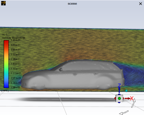
Limitations for LICs
The mouse-probe functionality (accessed by selecting the probe
 toolbar icon) is not available for LICs plots.
Note: Before creating an LIC plot, you must create a plane surface for the LIC plot. Refer to Plane Surfaces for additional information on creating plane surfaces.
To create an LIC plot:
Right-click LICs in the Outline View tree and select New....
Results
→ Graphics
→ LICs New...
 (Optional) Enter a Name for the LIC object.
Specify the field variable you want to use to color the LIC results by selecting the category and variable from the Color by drop-down lists.
Specify whether the vectors represent velocity or relative velocity using the Vectors of drop-down list.
Select the planar surface(s) where you want the LIC results displayed in the Plane Surfaces list.
You can click to open the Plane Surface Dialog Box in the Fluent User's Guide.
(Optional) Specify the display state that you want associated with this object. Refer to Controlling the Display State and Modifying the View for additional information.
Specify whether you want the range to be Global, Local to the selected surface(s), or Custom.
Set the Texture Size slider to control the size (in 100's of pixels) of the texture image used in the convolution.
Click .
Click if you are happy with the plot and want it to persist with the case file.
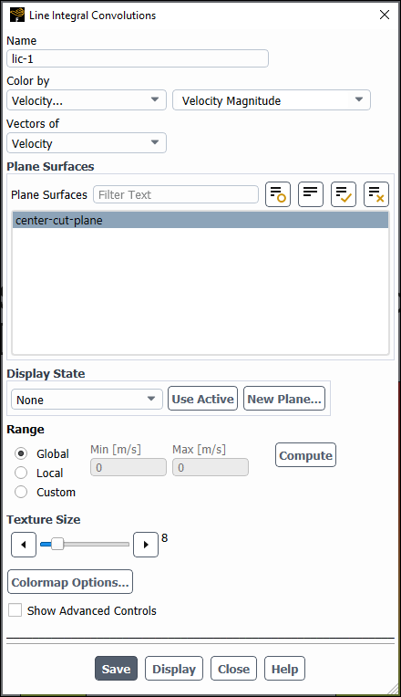
Scenes can be used to display multiple graphics plots within a single window. For example, you could overlay contours of pressure across a valve with velocity vectors and the mesh at the same location. Scenes allow you to modify the transparency of each plot so that you can emphasize a particular plot or view.
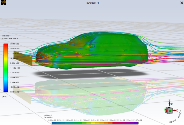
Note: You can use the "make selected faces transparent" toolbar button (![]() ) to quickly and temporarily make surfaces transparent.
However, if you want the applied transparency to persist with the case file,
then you should use the scene object described in this section.
) to quickly and temporarily make surfaces transparent.
However, if you want the applied transparency to persist with the case file,
then you should use the scene object described in this section.
You can plot a scene made up of multiple graphics objects using the Figure 40.50: The Scene Dialog Box.
![]() Results → Scene
Results → Scene
![]() New...
New...
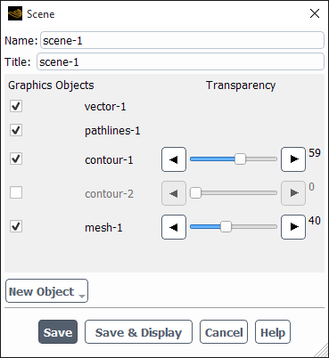
The basic steps for creating a scene:
(Optional) Enter a Name for the scene.
(Optional) Enter a Title for the scene, which will appear in the graphics window tab where the scene is displayed.
Select the Graphics Objects that you want to include in the scene. If you want to include additional mesh, contour, vector, or pathline plots in the scene, create them from the New Object drop-down list.
Note that pathlines with the XY Plot option enabled are not compatible with scenes.
(Optional) You can modify the transparency of the selected graphics objects using the Transparency slider. If the slider is completely to the right the object will be fully transparent.
Note: The transparency slider does not work on mesh surfaces rendered with realistic materials (List of Default Realistic Materials). If you want a surface colored by a material to appear more transparent, you can create a custom material with increased transparency using the Material Editor dialog box. Refer to Creating Custom Realistic Materials for additional information.
Click or .
Note: You can also save a scene from the current graphics window display by right-click > Save as Scene in the graphics window, as discussed in Quickly Coloring Surfaces by Field Variable Value.
Scene Colormaps
Once the scene is displayed, you can move the colormaps by left-click and drag. Colormaps can also be resized by dragging the corners of the box that appears when you hover over the colormap.
Tip: You can specify a different colormap scale for each graphic object to make it easier to determine the values that correspond to the displayed gradients (to do this, click Colormap Options... in the corresponding graphics object dialog box).
Sweep surfaces can be used when you want to examine the mesh, contours, or vectors on various sections of the domain without explicitly creating the corresponding surfaces. For example, if you want to display solution results for a 3D combustion chamber, instead of creating numerous surfaces at different cross-sections of the domain, you can use a sweep surface to view the variation of the flow and temperature throughout the chamber.
You can plot meshes, contours, or vectors on a sweep surface using the Sweep Surface Dialog Box (Figure 40.51: The Sweep Surface Dialog Box).
![]() Results → Animations → Sweep Surface
Results → Animations → Sweep Surface ![]() Edit...
Edit...
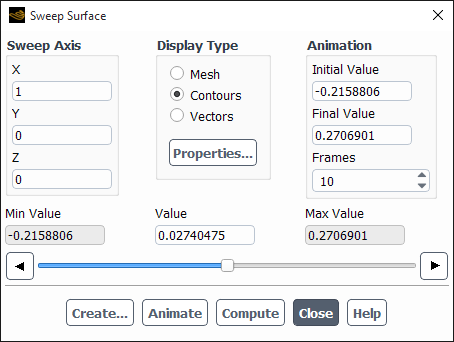
The basic steps for generating a mesh, contour, or vector plot using a sweep surface are as follows:
Under Sweep Axis, specify the (X, Y, Z) vector representing the axis along which the surface should be swept.
Click to update the Min Value and Max Value to reflect the extents of the domain along the specified axis.
Under Display Type, specify the type of display you want to see: Mesh, Contours, or Vectors. The first time that you select Contours or Vectors, Ansys Fluent will open the Contours Dialog Box or the Vectors Dialog Box so you can modify the settings for the display. To make subsequent modifications to the display settings, click to open the Contours Dialog Box or Vectors Dialog Box.
Move the slider under Value (which indicates the value of x, y, or z) to move the sweep surface through the domain along the specified Sweep Axis. Ansys Fluent will update the mesh, contour, or vector display when you release the slider. You can also enter a position in the Value field and press Enter to update the display.
If you want to save the currently displayed sweep surface so that you can use it for a different type of plot (for example, a pathlines plot or an XY plot) or combine it with displays on other surfaces, click to open the Create Surface Dialog Box (Figure 40.52: The Create Surface Dialog Box). Enter the Surface Name and click .
The surface that is created is an isosurface based on the mesh coordinates; the contour or vector settings are not stored in the surface.
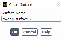
You can also animate the sweep surface display, as described below, rather than moving the slide bar yourself.
The steps for animating a sweep surface display are as follows:
Specify the Sweep Axis and Display Type as described above.
Under Animation, enter the Initial Value and Final Value for the animation. These values correspond to the minimum and maximum values along the Sweep Axis for which you want to animate the display.
Specify the number of Frames you want to see in the animation.
Click .
There may be situations where displaying graphics on a local machine is not practical. Therefore, you may decide to hide (or disable) the graphics display window.
To disable the graphics display window when starting Ansys Fluent from the command line, you can specify the driver as null:
fluent -driver null
For an Ansys Fluent session that is already in progress, the graphics window display can be disabled using the following text command:
display → set →
rendering-options →
driver → null
Important: All graphics windows must be closed prior to invoking the previous text command.
If the graphics window display is disabled, you can continue to save graphics using the Save Picture option, as described in Saving Picture Files. Note that the speed at which the graphics are saved may be significantly slower with the driver set to null, and the saved graphics files may not be identical to those saved when the graphics window display is enabled.
For an Ansys Fluent session that is already in progress, perform the following steps to re-enable a graphics window display that had been previously disabled:
Enter the following text command:
display→set→rendering-options→driverPress the Enter key at the
driver>prompt to display the available drivers.Enter an appropriate driver, such as
opengl.
If any graphics windows are open (which are not visible to you), Ansys Fluent will prompt you to close all open windows. You can close them using the following Scheme command:
(close-all-open-windows)
and then retype the text command to enable the graphics windows.
Important: If you happen to be logged on to a machine remotely,
then some drivers may not work on your system. Use x11
(for Linux) or msw (for Windows) instead to enable your
graphics windows.