


Boundary conditions consist of external, internal, and periodic boundaries. Most of the boundary conditions are discussed in the sections that follow.
- 7.4.1. Flow Inlet and Exit Boundary Conditions
- 7.4.2. Using Flow Boundary Conditions
- 7.4.3. Pressure Inlet Boundary Conditions
- 7.4.4. Velocity Inlet Boundary Conditions
- 7.4.5. Mass-Flow Inlet Boundary Conditions
- 7.4.6. Mass-Flow Outlet Boundary Conditions
- 7.4.7. Inlet Vent Boundary Conditions
- 7.4.8. Intake Fan Boundary Conditions
- 7.4.9. Pressure Outlet Boundary Conditions
- 7.4.10. Pressure Far-Field Boundary Conditions
- 7.4.11. Outflow Boundary Conditions
- 7.4.12. Outlet Vent Boundary Conditions
- 7.4.13. Exhaust Fan Boundary Conditions
- 7.4.14. Degassing Boundary Conditions
- 7.4.15. Wall Boundary Conditions
- 7.4.16. Perforated Wall Boundary Conditions
- 7.4.17. Symmetry Boundary Conditions
- 7.4.18. Periodic Boundary Conditions
- 7.4.19. Axis Boundary Conditions
- 7.4.20. Fan Boundary Conditions
- 7.4.21. Radiator Boundary Conditions
- 7.4.22. Porous Jump Boundary Conditions
You can find details about the following types here:
interface zones: Using Sliding Meshes
interior zones: Interior Dialog Box
overset zones: Overset Meshes
RANS/LES interface zones: Setting Up the Embedded Large Eddy Simulation (ELES) Model
Note: By default, boundaries are grouped by type, but you also have the option of grouping them by:
Alphabetical (List View)
Name
Cell Zone (Adjacency)
To change the grouping, right-click the Boundary Conditions branch in the Outline View tree and select Group By/List View or Name or Adjacency.
![]() Setup → Boundary Conditions
Setup → Boundary Conditions ![]() Group
By → List View | Name | Adjacency
Group
By → List View | Name | Adjacency
You can set the default boundary organization method using the Group boundary conditions by drop-down in Preferences (Appearance branch).
![]() File → Preferences
File → Preferences
Ansys Fluent has a wide range of boundary conditions that permit flow to enter and exit the solution domain. To help you select the most appropriate boundary condition for your application, this section includes descriptions of how each type of condition is used, and what information is needed for each one. Recommendations for determining inlet values of the turbulence parameters are also provided.
This section provides an overview of flow boundaries in Ansys Fluent and how to use them.
Ansys Fluent provides 12 types of boundary zone types for the specification of flow inlets and exits: velocity inlet, pressure inlet, mass-flow inlet, mass-flow outlet, pressure outlet, pressure far-field, outflow, inlet vent, intake fan, outlet vent, exhaust fan, and degassing.
The inlet and exit boundary condition options in Ansys Fluent are as follows:
Velocity inlet boundary conditions are used to define the velocity and scalar properties of the flow at inlet boundaries.
Pressure inlet boundary conditions are used to define the total pressure and other scalar quantities at flow inlets.
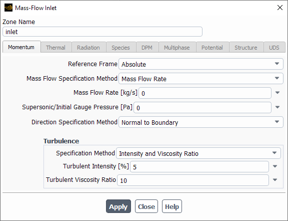
Mass-flow inlet boundary conditions are used in compressible flows to prescribe a mass flow rate at an inlet. It is not necessary to use mass-flow inlets in incompressible flows because when density is constant, velocity inlet boundary conditions will fix the mass flow. Like pressure and velocity inlets, other inlet scalars are also prescribed.
Pressure outlet boundary conditions are used to define the static pressure at flow outlets (and also other scalar variables, in case of backflow). The use of a pressure outlet boundary condition instead of an outflow condition often results in a better rate of convergence when backflow occurs during iteration.
Pressure far-field boundary conditions are used to model a free-stream compressible flow at infinity, with free-stream Mach number and static conditions specified. This boundary type is available only for compressible flows.
Outflow boundary conditions are used to model flow exits where the details of the flow velocity and pressure are not known prior to solution of the flow problem. They are appropriate where the exit flow is close to a fully developed condition, as the outflow boundary condition assumes a zero streamwise gradient for all flow variables except pressure. They are not appropriate for compressible flow calculations.
Inlet vent boundary conditions are used to model an inlet vent with a specified loss coefficient, flow direction, and ambient (inlet) total pressure and temperature.
Intake fan boundary conditions are used to model an external intake fan with a specified pressure jump, flow direction, and ambient (intake) total pressure and temperature.
Outlet vent boundary conditions are used to model an outlet vent with a specified loss coefficient and ambient (discharge) static pressure and temperature.
Exhaust fan boundary conditions are used to model an external exhaust fan with a specified pressure jump and ambient (discharge) static pressure.
Degassing boundary conditions are used to model a free surface through which dispersed gas bubbles are allowed to escape, but the continuous liquid phase is not. A typical application is a bubble column in which you want to reduce computational cost by not including the freeboard region in the simulation. The degassing boundary condition is only available for two-phase liquid-gas flows using the Eulerian multiphase model.
When the flow enters the domain at an inlet, outlet, or far-field boundary, Ansys Fluent requires specification of transported turbulence quantities. This section describes which quantities are needed for specific turbulence models and how they must be specified. It also provides guidelines for the most appropriate way of determining the inflow boundary values.
If it is important to accurately represent a boundary layer or fully-developed turbulent flow at the inlet, you should ideally set the turbulence quantities by creating a profile file (see Profiles) from experimental data or empirical formulas. If you have an analytical description of the profile, rather than data points, you can either use this analytical description to create a profile file, or create a user-defined function to provide the inlet boundary information. (See the Fluent Customization Manual for information on user-defined functions.)
Once you have created the profile function, you can use it as described below:
Spalart-Allmaras model: Choose Modified Turbulent Viscosity or Turbulent Viscosity Ratio in the Turbulence Specification Method drop-down list and select the appropriate profile name in the drop-down list next to Turbulent Viscosity or Turbulent Viscosity Ratio. Ansys Fluent computes the boundary value for the modified turbulent viscosity,
 , by combining
  with the appropriate values of density and molecular viscosity.
 -
-  models: Choose K and Epsilon in the Turbulence Specification
Method drop-down list and select the appropriate profile names in the drop-down lists next to
Turbulent Kinetic Energy and Turbulent Dissipation Rate.
models: Choose K and Epsilon in the Turbulence Specification
Method drop-down list and select the appropriate profile names in the drop-down lists next to
Turbulent Kinetic Energy and Turbulent Dissipation Rate. -
-  models: Choose K and Omega in the Turbulence Specification
Method drop-down list and select the appropriate profile names in the drop-down lists next to
Turbulent Kinetic Energy and Specific Dissipation Rate.
models: Choose K and Omega in the Turbulence Specification
Method drop-down list and select the appropriate profile names in the drop-down lists next to
Turbulent Kinetic Energy and Specific Dissipation Rate. -based Reynolds stress models: Choose K and Epsilon in the Turbulence
Specification Method drop-down list and select the appropriate profile names in the drop-down lists
next to Turbulent Kinetic Energy and Turbulent Dissipation Rate. Choose
Reynolds-Stress Components in the Reynolds-Stress Specification Method
drop-down list and select the appropriate profile name in the drop-down list next to each of the individual
Reynolds-stress components.
-based Reynolds stress models: Choose K and Epsilon in the Turbulence
Specification Method drop-down list and select the appropriate profile names in the drop-down lists
next to Turbulent Kinetic Energy and Turbulent Dissipation Rate. Choose
Reynolds-Stress Components in the Reynolds-Stress Specification Method
drop-down list and select the appropriate profile name in the drop-down list next to each of the individual
Reynolds-stress components. -based Reynolds stress models: Choose K and Omega in the Turbulence
Specification Method drop-down list and select the appropriate profile names in the drop-down lists
next to Specific Dissipation Rate. Choose Reynolds-Stress Components in the
Reynolds-Stress Specification Method drop-down list and select the appropriate profile name
in the drop-down list next to each of the individual Reynolds-stress components.
-based Reynolds stress models: Choose K and Omega in the Turbulence
Specification Method drop-down list and select the appropriate profile names in the drop-down lists
next to Specific Dissipation Rate. Choose Reynolds-Stress Components in the
Reynolds-Stress Specification Method drop-down list and select the appropriate profile name
in the drop-down list next to each of the individual Reynolds-stress components.
In some situations, it is appropriate to specify a uniform value of the turbulence quantity at the boundary where inflow occurs. Examples are fluid entering a duct, far-field boundaries, or even fully-developed duct flows where accurate profiles of turbulence quantities are unknown.
In most turbulent flows, higher levels of turbulence are generated within shear layers than enter the domain at flow boundaries, making the result of the calculation relatively insensitive to the inflow boundary values. Nevertheless, caution must be used to ensure that boundary values are not so unphysical as to contaminate your solution or impede convergence. This is particularly true of external flows where unphysically large values of effective viscosity in the free stream can “swamp” the boundary layers.
You can use the turbulence specification methods described above to enter uniform constant values instead of profiles.
Alternatively, you can specify the turbulence quantities in terms of more convenient quantities such as turbulence intensity,
turbulent viscosity ratio, hydraulic diameter, and turbulence length scale. The default Turbulence Specification Method is set
to Turbulent Viscosity Ratio (for the Spalart-Allmaras model) or Intensity and Viscosity
Ratio (for the  -
-  models, the
  -
-  models, or the RSM). These quantities are discussed further in the following sections.
The turbulence intensity,  , is defined as the ratio of the root-mean-square of the velocity fluctuations,
  , to the mean flow velocity,
  .
.
A turbulence intensity of 1% or less is generally considered low and turbulence intensities greater than 10% are considered high. Ideally, you will have a good estimate of the turbulence intensity at the inlet boundary from external, measured data. For example, if you are simulating a wind-tunnel experiment, the turbulence intensity in the free stream is usually available from the tunnel characteristics. In modern low-turbulence wind tunnels, the free-stream turbulence intensity may be as low as 0.05%.
For internal flows, the turbulence intensity at the inlets is totally dependent on the upstream history of the flow. If the
flow upstream is under-developed and undisturbed, you can use a low turbulence intensity. If the flow is fully developed, the
turbulence intensity may be as high as a few percent. The turbulence intensity at the core of a fully-developed duct flow can
be derived from an empirical correlation by Blasius for pipe flows (see Chapter 20 Equations (20-4) and (20-5) in [137]), using the additional estimation of the RMS velocity fluctuation at the pipe core  :
:
 | (7–72) |
At a Reynolds number of 50,000, for example, the turbulence intensity will be 4%, according to this formula.
The default value for turbulence intensity is 5% (medium intensity).
The turbulence length scale,  , is a physical quantity related to the size of the large eddies that contain the energy in turbulent
flows.
, is a physical quantity related to the size of the large eddies that contain the energy in turbulent
flows.
In fully-developed duct flows,  is restricted by the size of the duct, since the turbulent eddies cannot be larger than the duct. An
approximate relationship between
is restricted by the size of the duct, since the turbulent eddies cannot be larger than the duct. An
approximate relationship between  and the physical size of the duct is
 | (7–73) |
where  is the relevant dimension of the duct and
  ensures consistency with the definition of the turbulent length scales for one- and two-equation turbulence
models. The factor of 0.07 is based on the maximum value of the mixing length in fully-developed turbulent pipe flow, where
ensures consistency with the definition of the turbulent length scales for one- and two-equation turbulence
models. The factor of 0.07 is based on the maximum value of the mixing length in fully-developed turbulent pipe flow, where
 is the diameter of the pipe. In a channel of non-circular cross-section, you can base
  on the hydraulic diameter.
If the turbulence derives its characteristic length from an obstacle in the flow, such as a perforated plate, it is more appropriate to base the turbulence length scale on the characteristic length of the obstacle rather than on the duct size.
It should be noted that the relationship of Equation 7–73, which relates a physical dimension
( ) to the turbulence length scale (
 ), is not necessarily applicable to all situations. For most cases, however, it is a suitable
approximation.
), is not necessarily applicable to all situations. For most cases, however, it is a suitable
approximation.
Guidelines for choosing the characteristic length  or the turbulence length scale
  for selected flow types are listed below:
For fully-developed internal flows, choose the Intensity and Hydraulic Diameter specification method and specify the hydraulic diameter
 in the Hydraulic Diameter field.
For flows downstream of turning vanes, perforated plates, and so on, choose the Intensity and Length Scale method and specify the characteristic length of the flow opening for
 in the Turbulent Length Scale field.
For wall-bounded flows in which the inlets involve a turbulent boundary layer, choose the Intensity and Length Scale method and use the boundary-layer thickness,
 , to compute the turbulence length scale,
  , from
  . Enter this value for
  in the Turbulence Length Scale field.
The turbulent viscosity ratio,  , is directly proportional to the turbulent Reynolds number (
 ).
).  is large (on the order of 100 to 1000) in high-Reynolds-number boundary layers, shear layers, and
fully-developed duct flows. However, at the free-stream boundaries of most external flows,
is large (on the order of 100 to 1000) in high-Reynolds-number boundary layers, shear layers, and
fully-developed duct flows. However, at the free-stream boundaries of most external flows,  is fairly small. Typically, the turbulence parameters are set so that
  . For internal flows values up to 100 are sensible for the turbulent viscosity ratio,
  . The default value for the turbulent viscosity ratio is set to 10.
To specify quantities in terms of the turbulent viscosity ratio, you can choose Turbulent Viscosity
Ratio (for the Spalart-Allmaras model) or Intensity and Viscosity Ratio (for the
 -
-  models, the
  -
-  models, or the RSM). The default value for the turbulence intensity is set to 5% (medium intensity)
and the turbulent viscosity ratio,
models, or the RSM). The default value for the turbulence intensity is set to 5% (medium intensity)
and the turbulent viscosity ratio,  , has a default value of 10.
To obtain the values of transported turbulence quantities from more convenient quantities such as  ,
,  , or
, or  , you must typically resort to an empirical relations in addition to the formal definitions of these
quantities. Several formal definitions and useful empirical relations, most of which are used within Ansys Fluent, are presented
below.
, you must typically resort to an empirical relations in addition to the formal definitions of these
quantities. Several formal definitions and useful empirical relations, most of which are used within Ansys Fluent, are presented
below.
To obtain the modified turbulent viscosity,  , for the Spalart-Allmaras model from the turbulence intensity,
  , and length scale,
  , the following equation can be used. Note that this equation assumes that there is no viscous damping, that
is,
, the following equation can be used. Note that this equation assumes that there is no viscous damping, that
is,  (see Modeling the Turbulent Viscosity in the Theory Guide).
 | (7–74) |
This formula is also used in Ansys Fluent if you select the Intensity and Hydraulic Diameter
specification method with the Spalart-Allmaras model. In this case,  is obtained from Equation 7–73.
  ensures consistency with the definition of the eddy viscosity for
  -
-  and
and  -
-  turbulence models. The value of
  is 0.09.
When using a moving reference frame, be aware of the order of the conversion operations applied to the inlet velocity and to
the turbulence quantities, which is explained in the next section. It concerns the values of  in Equation 7–74.
The relationship between the turbulent kinetic energy,  , and turbulence intensity,
  , is
, is
 | (7–75) |
where is the magnitude of the mean flow velocity.
This relationship is used in Ansys Fluent whenever the Intensity and Hydraulic Diameter,
Intensity and Length Scale, or Intensity and Viscosity Ratio method is used instead
of specifying explicit values for  and
and  or .
or .
Important: The reference frame for the mean flow velocity in Equation 7–75
corresponds to the Velocity Formulation selected in the General Task Page, see also Choosing the Relative or Absolute Velocity Formulation. When selecting the Reference Frame in any of the inlet boundary condition dialog boxes
(see, for example, Figure 7.37: The Velocity Inlet Dialog Box for the Velocity Inlet Boundary Conditions), be aware
that the specified inlet velocity is first converted to the selected Velocity Formulation and then applied to compute the
turbulent kinetic energy from turbulence intensity using Equation 7–75. If an inlet boundary type does
not require the inlet velocity specification (for example, Pressure Inlet Boundary Conditions), then in Equation 7–75 is the current local solution velocity magnitude, which corresponds
to the selected Velocity Formulation.
If you know the turbulence length scale,  , you can determine
  from the relationship
 | (7–76) |
The determination of  was discussed previously.
This relationship is used in Ansys Fluent whenever the Intensity and Hydraulic Diameter or
Intensity and Length Scale method is used instead of specifying explicit values for  and
and  .
.
The value of  can be obtained from the turbulent viscosity ratio
  and
and  using the following relationship:
 | (7–77) |
where  is an empirical constant specified in the turbulence model.
This relationship is used in Ansys Fluent whenever the Intensity and Viscosity Ratio method is used
instead of specifying explicit values for  and
and  .
.
If you are simulating a wind-tunnel situation in which the model is mounted in the test section downstream of a mesh and/or
wire mesh screens, you can choose a value of  such that
 | (7–78) |
where  is the approximate decay of
  you want to have across the flow domain (say, 10% of the inlet value of
  ),
),  is the free-stream velocity, and
  is the streamwise length of the flow domain. Equation 7–78 is a linear approximation
to the power-law decay observed in high-Reynolds-number isotropic turbulence. Its basis is the exact equation for
is the streamwise length of the flow domain. Equation 7–78 is a linear approximation
to the power-law decay observed in high-Reynolds-number isotropic turbulence. Its basis is the exact equation for
 in decaying turbulence,
  .
.
If you use this method to estimate  , you should also check the resulting turbulent viscosity ratio
  to make sure that it is not too large, using Equation 7–77.
Although this method is not used internally by Ansys Fluent, you can use it to derive a constant free-stream value of
 that you can then specify directly by choosing K and Epsilon in the
Turbulence Specification Method drop-down list. In this situation, you will typically determine
that you can then specify directly by choosing K and Epsilon in the
Turbulence Specification Method drop-down list. In this situation, you will typically determine
 from
from  using Equation 7–75.
If you know the turbulence length scale,  , you can determine
  from the relationship
 | (7–79) |
where  is an empirical constant specified in the turbulence model. The determination of
  was discussed previously.
This relationship is used in Ansys Fluent whenever the Intensity and Hydraulic Diameter or
Intensity and Length Scale method is used instead of specifying explicit values for  and
and  .
.
The value of  can be obtained from the turbulent viscosity ratio
  and
and  using the following relationship:
 | (7–80) |
This relationship is used in Ansys Fluent whenever the Intensity and Viscosity Ratio method is used
instead of specifying explicit values for  and
and  .
.
When the RSM is used, if you do not specify the values of the Reynolds stresses explicitly at the inlet using the
Reynolds-Stress Components option in the Reynolds-Stress Specification Method
drop-down list, they are approximately determined from the specified values of  . The turbulence is assumed to be isotropic such that
 | (7–81) |
and
 | (7–82) |
(no summation over the index  ).
).
Ansys Fluent will use this method if you select K or Turbulence Intensity in the Reynolds-Stress Specification Method drop-down list.
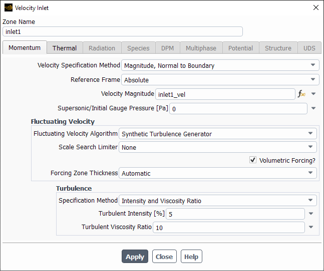
When using Scale Resolving Simulations (SAS, DES, SDES, SBES, and LES models), it is possible to specify unsteady Fluctuating Velocity at velocity and pressure inlets to generate realistic turbulent content. Therefore, additional input is required for velocity and pressure inlets such as the choice of Fluctuating Velocity Algorithm and corresponding parameters (as shown in Figure 7.34: Specifying Inlet Turbulence for Scale Resolving Simulation). The available methods along with their options are described in Inlet Boundary Conditions for Scale Resolving Simulations in the Fluent Theory Guide. Note that even though some LES models do not require specification of the Turbulence parameters at the boundary, it is required when a Fluctuating Velocity Algorithm is selected. Additional parameters available for the Fluctuating Velocity Algorithm are listed in Pressure Inlet Dialog Box and Velocity Inlet Dialog Box.
Pressure inlet boundary conditions are used to define the fluid pressure at flow inlets, along with all other scalar properties of the flow. They are suitable for both incompressible and compressible flow calculations. Pressure inlet boundary conditions can be used when the inlet pressure is known but the flow rate and/or velocity is not known. This situation may arise in many practical situations, including buoyancy-driven flows. Pressure inlet boundary conditions can also be used to define a “free” boundary in an external or unconfined flow.
For an overview of flow boundaries, see Flow Inlet and Exit Boundary Conditions.
You will enter the following information for a pressure inlet boundary:
type of reference frame
total (stagnation) pressure
total (stagnation) temperature
flow direction
static pressure
turbulence parameters (for turbulent calculations)
radiation parameters (for calculations using the P-1, DTRM, DO, surface-to-surface, or MC models)
chemical species mass or mole fractions (for species calculations)
mixture fraction and variance (for non-premixed or partially premixed combustion calculations)
progress variable (for premixed or partially premixed combustion calculations)
discrete phase boundary conditions (for discrete phase calculations)
multiphase boundary conditions (for general multiphase calculations)
open channel flow parameters (for open channel flow calculations using the VOF multiphase model)
acoustic wave model settings
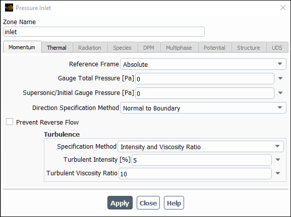
All values are entered in the Pressure Inlet Dialog Box (Figure 7.35: The Pressure Inlet Dialog Box), which is opened from the Boundary Conditions task page (as described in Setting Cell Zone and Boundary Conditions ). Note that open channel boundary condition inputs are described in Modeling Open Channel Flows, and acoustic wave model settings are described in Boundary Acoustic Wave Models.
When gravitational acceleration is activated in the Operating Conditions dialog box (accessed from
the Boundary Conditions task page), the pressure field (including all pressure inputs) will include
the hydrostatic head. This is accomplished by redefining the pressure in terms of a modified pressure that includes the
hydrostatic head (denoted  ) as follows:
 | (7–83) |
where  is a constant operating density,
  is the gravity vector (also a constant), and
 | (7–84) |
is the position vector. Noting that
 | (7–85) |
it follows that
 | (7–86) |
The substitution of this relation in the momentum equation gives pressure gradient and gravitational body force terms of the form
 | (7–87) |
where  is the fluid density. Therefore, if the fluid density is constant, we can set the operating density
 equal to the fluid density, thereby eliminating the body force term. If the fluid density is not
constant (for example, density is given by the ideal gas law), then the operating density should be chosen to be
representative of the average or mean density in the fluid domain, so that the body force term is small.
equal to the fluid density, thereby eliminating the body force term. If the fluid density is not
constant (for example, density is given by the ideal gas law), then the operating density should be chosen to be
representative of the average or mean density in the fluid domain, so that the body force term is small.
An important consequence of this treatment of the gravitational body force is that your inputs of pressure (now defined
as  ) should not include hydrostatic pressure differences. Moreover, reports of static and total pressure
will not show any influence of the hydrostatic pressure. See Buoyancy-Driven Flows and Natural Convection for additional
information.
) should not include hydrostatic pressure differences. Moreover, reports of static and total pressure
will not show any influence of the hydrostatic pressure. See Buoyancy-Driven Flows and Natural Convection for additional
information.
Enter the value for total pressure in the Gauge Total Pressure field in the Pressure Inlet dialog box. Total temperature is set in the Thermal tab, in the Total Temperature field.
Remember that the total pressure value is the gauge pressure with respect to the operating pressure defined in the Operating Conditions Dialog Box. Total pressure for an incompressible fluid is defined as
 | (7–88) |
and for a compressible fluid of constant  as
as
 | (7–89) |
|
where |
|
|
| |
|
M = Mach number | |
|
|


If you are modeling axisymmetric swirl,  in Equation 7–88 will include the swirl component.
The Total Temperature, Gauge Total Pressure, and flow directions are in absolute or relative to the adjacent cell zone reference frames, based on the Reference Frame setting in the Pressure Inlet dialog box.
If the cell zone adjacent to a pressure inlet is defined as a moving reference frame zone, and you are using the pressure-based solver, the velocity in Equation 7–88 (or the Mach number in Equation 7–89) will be absolute or relative to the mesh velocity, depending on whether or not the Absolute velocity formulation is enabled in the General task page. For the density-based solver, the Absolute velocity formulation is always used; hence, the velocity in Equation 7–88 (or the Mach number in Equation 7–89) is always the Absolute velocity.
For the Eulerian multiphase model, the total temperature, and velocity components must be specified for the individual phases. The Reference Frame (Relative to Adjacent Cell Zone or Absolute) for each of the phases is the same as the reference frame selected for the mixture phase. Note that the total pressure values must be specified in the mixture phase.
Important:
If the flow is incompressible, then the temperature assigned in the Pressure Inlet dialog box will be considered the static temperature.
For the mixture multiphase model, if a boundary allows a combination of compressible and incompressible phases to enter the domain, then the temperature assigned in the Pressure Inlet dialog box will be considered the static temperature at that boundary. If a boundary allows only a compressible phase to enter the domain, then the temperature assigned in the Pressure Inlet dialog box will be taken as the total temperature (relative/absolute) at that boundary. The total temperature will depend on the Reference Frame option selected in the Pressure Inlet dialog box.
For the VOF multiphase model, if a boundary allows a compressible phase to enter the domain, then the temperature assigned in the Pressure Inlet dialog box will be considered the total temperature at that boundary. The total temperature (relative/absolute) will depend on the Reference Frame option chosen in the dialog box. Otherwise, the temperature assigned to the boundary will be considered the static temperature at the boundary.
For the Eulerian multiphase model, if a boundary allows a mixture of compressible and incompressible phases in the domain, then the temperature of each of the phases will be the total or static temperature, depending on whether the phase is compressible or incompressible.
Total temperature (relative/absolute) will depend on the Reference Frame option chosen in the Pressure Inlet dialog box.
The flow direction is defined as a unit vector ( ) which is aligned with the local velocity vector,
  . This can be expressed simply as
 | (7–90) |
Important: For the inputs in Ansys Fluent, the flow direction  need not be a unit vector, as it will be automatically normalized before it is applied.
Important: For a moving reference frame, the relative flow direction  is defined in terms of the relative velocity,
  . Thus,
 | (7–91) |
You can define the flow direction at a pressure inlet explicitly, or you can define the flow to be normal to the
boundary. If you choose to specify the direction vector, you can set either the (Cartesian)  ,
,  , and
, and  components, or the (cylindrical) radial, tangential, and axial components.
For moving zone problems calculated using the pressure-based solver, the flow direction will be absolute or relative to the mesh velocity, depending on whether or not the Absolute velocity formulation is selected in the General task page. For the density-based solver, the flow direction will always be in the absolute frame.
The procedure for defining the flow direction is as follows (refer to Figure 7.35: The Pressure Inlet Dialog Box):
Specify the flow direction by selecting Direction Vector or Normal to Boundary in the Direction Specification Method drop-down list.
If you selected Normal to Boundary in step 1 and you are modeling axisymmetric swirl, enter the appropriate value for the Tangential-Component of Flow Direction. If you chose Normal to Boundary and your geometry is 3D or 2D without axisymmetric swirl, there are no additional inputs for flow direction.
If you selected Direction Vector in step 1, and your geometry is 3D, choose Cartesian (X, Y, Z), Cylindrical(Radial, Tangential, Axial), Local Cylindrical (Radial, Tangential, Axial), or Local Cylindrical Swirl from the Coordinate System drop-down list. Some notes on these selections are provided below:
The Cartesian coordinate option is based on the Cartesian coordinate system used by the geometry. Enter appropriate values for the X, Y, and Z-Component of Flow Direction.
The Cylindrical coordinate system uses the axial, radial, and tangential components based on the following coordinate systems:
For problems involving a single cell zone, the coordinate system is defined by the rotation axis and origin specified in the Fluid Dialog Box.
For problems involving multiple zones (for example, multiple reference frames or sliding meshes), the coordinate system is defined by the rotation axis specified in the Fluid (or Solid) dialog box for the fluid (or solid) zone that is adjacent to the inlet.
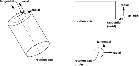
For all of the above definitions of the cylindrical coordinate system, positive radial velocities point radially outward from the rotation axis, positive axial velocities are in the direction of the rotation axis vector, and positive tangential velocities are based on the right-hand rule using the positive rotation axis (see Figure 7.36: Cylindrical Velocity Components in 3D, 2D, and Axisymmetric Domains).
The Local Cylindrical coordinate system allows you to define a coordinate system specifically for the inlet. When you use the local cylindrical option, you will define the coordinate system right here in the Pressure Inlet dialog box. The local cylindrical coordinate system is useful if you have several inlets with different rotation axes. Enter appropriate values for the Axial, Radial, and Tangential-Component of Flow Direction, and then specify the X, Y, and Z components of the Axis Origin and Axis Direction.
The Local Cylindrical Swirl coordinate system option allows you to define a coordinate system specifically for the inlet where the total pressure, swirl velocity, and the components of the velocity in the axial and radial planes are specified. Enter appropriate values for the Axial and Radial-Component of Flow Direction, and the Tangential-Velocity. Specify the X, Y, and Z components of the Axis Origin and Axis Direction. It is recommended that you start your simulation with a smaller swirl velocity and then progressively increase the velocity to obtain a stable solution.
Important: Local Cylindrical Swirl should not be used for open channel boundary conditions and on the mixing plane boundaries while using the mixing plane model.
If you selected Direction Vector in step 1, and your geometry is 2D, define the vector components as follows:
For a 2D planar geometry, enter appropriate values for the X, Y, and Z-Component of Flow Direction.
For a 2D axisymmetric geometry, enter appropriate values for the Axial, Radial-Component of Flow Direction.
For a 2D axisymmetric swirl geometry, enter appropriate values for the Axial, Radial, and Tangential-Component of Flow Direction.
Figure 7.36: Cylindrical Velocity Components in 3D, 2D, and Axisymmetric Domains shows the vector components for these different coordinate systems.
The static pressure (termed the Supersonic/Initial Gauge Pressure) must be specified if the inlet flow is supersonic or if you plan to initialize the solution based on the pressure inlet boundary conditions. Solution initialization is discussed in Initializing the Solution.
Remember that the static pressure value you enter is relative to the operating pressure set in the Operating Conditions Dialog Box. Note the comments in Pressure Inputs and Hydrostatic Head regarding hydrostatic pressure.
The Supersonic/Initial Gauge Pressure is ignored by Ansys Fluent whenever the flow is subsonic, in which case it is calculated from the specified stagnation quantities. If you choose to initialize the solution based on the pressure-inlet conditions, the Supersonic/Initial Gauge Pressure will be used in conjunction with the specified stagnation pressure to compute initial values according to the isentropic relations (for compressible flow) or Bernoulli’s equation (for incompressible flow). Therefore, for a sub-sonic inlet it should generally be set based on a reasonable estimate of the inlet Mach number (for compressible flow) or inlet velocity (for incompressible flow).
When this option is selected, Fluent will erect artificial walls on the boundary mesh faces to prevent flow out of the domain. The artificial walls are removed when the flow is no longer leaving the domain and when a favorable pressure gradient is recovered at the boundary mesh faces.
When artificial walls are created, Fluent will print a message in the console window indicating the number of faces on which artificial walls have been erected and the equivalent area percentage of the boundary it represents.
Note: This feature is not available with multiphase flow.
For turbulent calculations, there are several ways in which you can define the turbulence parameters. Instructions for deciding which method to use and determining appropriate values for these inputs are provided in Determining Turbulence Parameters. Turbulence modeling in general is described in Modeling Turbulence.
The options available depend on which radiation model is active. For details, see Defining Boundary Conditions for Radiation.
If you are modeling species transport, you will set the species mass or mole fractions under Species Mole Fractions or Species Mass Fractions. For details, see Defining Cell Zone and Boundary Conditions for Species.
If you are using the non-premixed or partially premixed combustion model, you will set the Mean Mixture Fraction and Mixture Fraction Variance (and the Secondary Mean Mixture Fraction and Secondary Mixture Fraction Variance, if you are using two mixture fractions), as described in Defining Non-Premixed Boundary Conditions.
If you are using the premixed or partially premixed combustion model, you will set the Progress Variable, as described in Setting Boundary Conditions for the Progress Variable.
If you are modeling a discrete phase of particles, you can set the fate of particle trajectories at the pressure inlet. See Setting Boundary Conditions for the Discrete Phase for details.
If you are using the VOF, mixture, or Eulerian model for multiphase flow, you will need to specify volume fractions for secondary phases and (for some models) additional parameters. See Defining Multiphase Cell Zone and Boundary Conditions for details.
If you are using the VOF model for multiphase flow and modeling open channel flows, you will need to specify the Free Surface Level, Bottom Level, and additional parameters. See Modeling Open Channel Flows for details.
Default settings (in SI) for pressure inlet boundary conditions are as follows:
| Gauge Total Pressure | 0 |
| Supersonic/Initial Gauge Pressure | 0 |
| Total Temperature | 300 |
| Direction Specification Method | Normal to Boundary |
| Turbulent Intensity | 5% |
| Turbulent Viscosity Ratio | 10 |
The treatment of pressure inlet boundary conditions by Ansys Fluent can be described as a loss-free transition from stagnation conditions to the inlet conditions. For incompressible flows, this is accomplished by application of the Bernoulli equation at the inlet boundary. In compressible flows, the equivalent isentropic flow relations for an ideal gas are used.
When flow enters through a pressure inlet boundary, Ansys Fluent uses the boundary condition pressure you input as the
total pressure of the fluid at the inlet plane,  . In incompressible flow, the inlet total pressure and the static pressure,
  , are related to the inlet velocity via Bernoulli’s equation:
 | (7–92) |
With the resulting velocity magnitude and the flow direction vector you assigned at the inlet, the velocity components can be computed. The inlet mass flow rate and fluxes of momentum, energy, and species can then be computed as outlined in Calculation Procedure at Velocity Inlet Boundaries.
For incompressible flows, density at the inlet plane is either constant or calculated as a function of temperature and/or species mass/mole fractions, where the mass or mole fractions are the values you entered as an inlet condition.
If flow exits through a pressure inlet, the total pressure specified is used as the static pressure. For incompressible flows, total temperature is equal to static temperature.
In compressible flows, isentropic relations for an ideal gas are applied to relate total pressure, static pressure, and
velocity at a pressure inlet boundary. Your input of total pressure,  , at the inlet and the static pressure,
  , in the adjacent fluid cell are therefore related as
 | (7–93) |
where
 | (7–94) |
 = the speed of sound, and
  . Note that the operating pressure,
  , appears in Equation 7–93 because your boundary condition inputs are in terms of
pressure relative to the operating pressure. Given
, appears in Equation 7–93 because your boundary condition inputs are in terms of
pressure relative to the operating pressure. Given  and
and  , Equation 7–93 and Equation 7–94 are used to compute the
velocity magnitude of the fluid at the inlet plane. Individual velocity components at the inlet are then derived using the
direction vector components.
, Equation 7–93 and Equation 7–94 are used to compute the
velocity magnitude of the fluid at the inlet plane. Individual velocity components at the inlet are then derived using the
direction vector components.
For compressible flow, the density at the inlet plane is defined by the ideal gas law in the form
 | (7–95) |
For multi-species gas mixtures, the specific gas constant,  , is computed from the species mass or mole fractions,
  that you defined as boundary conditions at the pressure inlet boundary. The static temperature at the inlet,
 , is computed from your input of total temperature,
  , as
, as
 | (7–96) |
Velocity inlet boundary conditions are used to define the flow velocity, along with all relevant scalar properties of the flow, at flow inlets. In this case, the total (or stagnation) pressure is not fixed but will rise (in response to the computed static pressure) to whatever value is necessary to provide the prescribed velocity distribution. This boundary condition is applicable to incompressible and compressible flows.
Important: Use caution when specifying the velocity inlet boundary condition for a compressible fluid in internal flow modeling. If the flow path is completely choked with no secondary flow path for relief, the velocity inlet boundary condition is not recommended, as it can cause numerical instabilities. In this case, you should switch to the pressure inlet boundary condition or refrain from reaching operating conditions that choke the internal flow. The choking condition can happen in high speed supersonic and transonic flow.
In special instances, a velocity inlet may be used in Ansys Fluent to define the flow velocity at flow exits. (The scalar inputs are not used in such cases.) In such cases you must ensure that overall continuity is maintained in the domain.
For an overview of flow boundaries, see Flow Inlet and Exit Boundary Conditions.
You will enter the following information for a velocity inlet boundary:
type of reference frame
velocity magnitude and direction or velocity components
swirl velocity (for 2D axisymmetric problems with swirl)
static pressure
temperature (for energy calculations)
outflow gauge pressure (for calculations with the density-based solver)
turbulence parameters (for turbulent calculations)
radiation parameters (for calculations using the P-1, DTRM, DO, surface-to-surface, or MC models)
chemical species mass or mole fractions (for species calculations)
mixture fraction and variance (for non-premixed or partially premixed combustion calculations)
progress variable (for premixed or partially premixed combustion calculations)
discrete phase boundary conditions (for discrete phase calculations)
multiphase boundary conditions (for general multiphase calculations)
acoustic wave model settings (see Boundary Acoustic Wave Models)
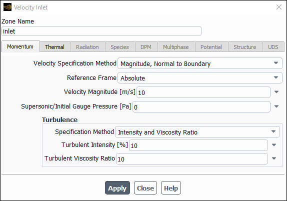
All values are entered in the Velocity Inlet Dialog Box (Figure 7.37: The Velocity Inlet Dialog Box), which is opened from the Boundary Conditions task page (as described in Setting Cell Zone and Boundary Conditions ). Note that acoustic wave model settings are described in Boundary Acoustic Wave Models.
You can define the inflow velocity by specifying the velocity magnitude and direction, the velocity components, or the velocity magnitude normal to the boundary. If the cell zone adjacent to the velocity inlet is moving (that is, if you are using a moving reference frame, multiple reference frames, or sliding meshes), you can specify either relative or absolute velocities. For axisymmetric problems with swirl in Ansys Fluent, you will also specify the swirl velocity.
The procedure for defining the inflow velocity is as follows:
Specify the flow direction by selecting Magnitude and Direction, Components, or Magnitude, Normal to Boundary in the Velocity Specification Method drop-down list.
If the cell zone adjacent to the velocity inlet is moving, you can choose to specify relative or absolute velocities by selecting Relative to Adjacent Cell Zone or Absolute in the Reference Frame drop-down list. If the adjacent cell zone is not moving, Absolute and Relative to Adjacent Cell Zone will be equivalent, so you need not visit the list.
If you are going to set the velocity magnitude and direction or the velocity components, and your geometry is 3D, choose Cartesian (X, Y, Z), Cylindrical (Radial, Tangential, Axial), or Local Cylindrical (Radial, Tangential, Axial) from the Coordinate System drop-down list. See Defining the Flow Direction for information about Cartesian, cylindrical, and local cylindrical coordinate systems.
Set the appropriate velocity parameters, as described below for each specification method.
If you selected Magnitude and Direction as the Velocity Specification Method in step 1 above, you will enter the magnitude of the velocity vector at the inflow boundary (the Velocity Magnitude) and the direction of the vector:
If your geometry is 2D non-axisymmetric, or you chose in step 3 to use the Cartesian coordinate system, you will define the X, Y, and (in 3D) Z-Component of Flow Direction.
If your geometry is 2D axisymmetric, or you chose in step 3 to use a Cylindrical coordinate system, enter the appropriate values of Radial, Axial, and (if you are modeling axisymmetric swirl or using cylindrical coordinates) Tangential-Component of Flow Direction.
If you chose in step 3 to use a Local Cylindrical coordinate system, enter appropriate values for the Axial, Radial, and Tangential-Component of Flow Direction, and then specify the X, Y, and Z components of the Axis Origin and the Axis Direction.
Figure 7.36: Cylindrical Velocity Components in 3D, 2D, and Axisymmetric Domains shows the vector components for these different coordinate systems.
If you selected Magnitude, Normal to Boundary as the Velocity Specification Method in step 1 above, you will enter the magnitude of the velocity vector at the inflow boundary (the Velocity Magnitude).
If you selected Components as the Velocity Specification Method in step 1 above, you will enter the components of the velocity vector at the inflow boundary as follows:
If your geometry is 2D non-axisymmetric, or you chose in step 3 to use the Cartesian coordinate system, you will define the X, Y, and (in 3D) Z-Velocity.
If your geometry is 2D axisymmetric without swirl, you will set the Radial and Axial-Velocity.
If your model is 2D axisymmetric with swirl, you will set the Axial, Radial, and Swirl-Velocity, and (optionally) the Angular Velocity, as described below.
If you chose in step 3 to use a Cylindrical coordinate system, you will set the Radial, Tangential, and Axial-Velocity, and (optionally) the Angular Velocity, as described below.
If you chose in step 3 to use a Local Cylindrical coordinate system, you will set the Radial, Tangential, and Axial-Velocity, and (optionally) the Angular Velocity, as described below, and then specify the X, Y, and Z component of the Axis Origin and the Axis Direction.
Important: Remember that positive values for  ,
,  , and
, and  velocities indicate flow in the positive
  ,
,  , and
, and  directions. If flow enters the domain in the negative
  direction, for example, you will need to specify a negative value for the
  velocity. The same holds true for the radial, tangential, and axial velocities. Positive radial
velocities point radially out from the axis, positive axial velocities are in the direction of the axis vector, and
positive tangential velocities are based on the right-hand rule using the positive axis.
velocity. The same holds true for the radial, tangential, and axial velocities. Positive radial
velocities point radially out from the axis, positive axial velocities are in the direction of the axis vector, and
positive tangential velocities are based on the right-hand rule using the positive axis.
If you chose Components as the Velocity Specification Method in step 1 above, and
you are modeling axisymmetric swirl, you can specify the inlet Angular Velocity  in addition to the Swirl-Velocity. Similarly, if you chose
Components as the Velocity Specification Method and you chose in step 3 to use a
Cylindrical or Local Cylindrical coordinate system, you can specify the inlet
Angular Velocity
in addition to the Swirl-Velocity. Similarly, if you chose
Components as the Velocity Specification Method and you chose in step 3 to use a
Cylindrical or Local Cylindrical coordinate system, you can specify the inlet
Angular Velocity  in addition to the Tangential-Velocity.
If you specify  ,
,  is computed for each face as
  , where
  is the radial coordinate in the coordinate system defined by the rotation axis and origin. If you specify
both the Swirl-Velocity and the Angular Velocity, or the
Tangential-Velocity and the Angular Velocity, Ansys Fluent will add
is the radial coordinate in the coordinate system defined by the rotation axis and origin. If you specify
both the Swirl-Velocity and the Angular Velocity, or the
Tangential-Velocity and the Angular Velocity, Ansys Fluent will add  and
and  to get the swirl or tangential velocity at each face.
The static pressure (termed the Supersonic/Initial Gauge Pressure) must be specified if the inlet flow is supersonic or if you plan to initialize the solution based on the velocity inlet boundary conditions. Solution initialization is discussed in Initializing the Solution.
The Supersonic/Initial Gauge Pressure is ignored by Ansys Fluent whenever the flow is subsonic. If you choose to initialize the flow based on the velocity inlet conditions, the Supersonic/Initial Gauge Pressure will be used in conjunction with the specified stagnation quantities to compute initial values according to isentropic relations.
Remember that the static pressure value you enter is relative to the operating pressure set in the Operating Conditions Dialog Box. Note the comments in Pressure Inputs and Hydrostatic Head
For calculations in which the energy equation is being solved, you will set the static temperature of the flow at the velocity inlet boundary in the Thermal tab in the Temperature field.
If you are using the density-based solver, you can specify an Outflow Gauge Pressure for a velocity inlet boundary. If the flow exits the domain at any face on the boundary, that face will be treated as a pressure outlet with the pressure prescribed in the Outflow Gauge Pressure field.
For turbulent calculations, there are several ways in which you can define the turbulence parameters. Instructions for deciding which method to use and determining appropriate values for these inputs are provided in Determining Turbulence Parameters. Turbulence modeling in general is described in Modeling Turbulence.
The options available depend on which radiation model is active. For details, see Defining Boundary Conditions for Radiation.
If you are modeling species transport, you will set the species mass or mole fractions under Species Mole Fractions or Species Mass Fractions. For details, see Defining Cell Zone and Boundary Conditions for Species.
If you are using the non-premixed or partially premixed combustion model, you will set the Mean Mixture Fraction and Mixture Fraction Variance (and the Secondary Mean Mixture Fraction and Secondary Mixture Fraction Variance, if you are using two mixture fractions), as described in Defining Non-Premixed Boundary Conditions.
If you are using the premixed or partially premixed combustion model, you will set the Progress Variable, as described in Setting Boundary Conditions for the Progress Variable.
If you are modeling a discrete phase of particles, you can set the fate of particle trajectories at the velocity inlet. See Setting Boundary Conditions for the Discrete Phase for details.
If you are using the VOF, mixture, or Eulerian model for multiphase flow, you will need to specify volume fractions for secondary phases and (for some models) additional parameters. See Defining Multiphase Cell Zone and Boundary Conditions for details.
Default settings (in SI) for velocity inlet boundary conditions are as follows:
| Temperature | 300 |
| Velocity Magnitude | 0 |
| X-Component of Flow Direction | 1 |
| Y-Component of Flow Direction | 0 |
| Z-Component of Flow Direction | 0 |
| X-Velocity | 0 |
| Y-Velocity | 0 |
|
Z-Velocity | 0 |
| Turbulent Intensity | 5% |
| Turbulent Viscosity Ratio | 10 |
| Outflow Gauge Pressure | 0 |
Ansys Fluent uses your boundary condition inputs at velocity inlets to compute the mass flow into the domain through the inlet and to compute the fluxes of momentum, energy, and species through the inlet. This section describes these calculations for the case of flow entering the domain through the velocity inlet boundary and for the less common case of flow exiting the domain through the velocity inlet boundary.
When your velocity inlet boundary condition defines flow entering the physical domain of the model, Ansys Fluent uses both the velocity components and the scalar quantities that you defined as boundary conditions to compute the inlet mass flow rate, momentum fluxes, and fluxes of energy and chemical species.
The mass flow rate entering a fluid cell adjacent to a velocity inlet boundary is computed as
 | (7–97) |
Note that only the velocity component normal to the control volume face contributes to the inlet mass flow rate.
Sometimes a velocity inlet boundary is used where flow exits the physical domain. This approach might be used, for example, when the flow rate through one exit of the domain is known or is to be imposed on the model.
Important: In such cases you must ensure that overall continuity is maintained in the domain.
In the pressure-based solver, when flow exits the domain through a velocity inlet boundary condition, Ansys Fluent uses the boundary velocity to compute the flow flux through the exit flow area and the viscous term in the momentum equation. The convection term in all equations including momentum uses upwind discretization and takes the values of the upstream cells.
In the density-based solver, if the flow exits the domain at any face on the boundary, that face will be treated as a pressure outlet with the pressure prescribed in the Outflow Gauge Pressure field.
Mass flow boundary conditions can be used in Ansys Fluent to provide a prescribed mass flow rate or mass flux distribution at an inlet. As with a velocity inlet, specifying the mass flux permits the total pressure to vary in response to the interior solution. This is in contrast to the pressure inlet boundary condition (see Pressure Inlet Boundary Conditions), where the total pressure is fixed while the mass flux varies. The mass-flow inlet is applicable to incompressible and compressible flows.
Important: Use caution when specifying the mass-flow inlet boundary condition for a compressible fluid in internal flow modeling. If the flow path is completely choked with no secondary flow path for relief, the mass-flow inlet boundary condition is not recommended, as it can cause numerical instabilities. In this case, you should switch to the pressure inlet boundary condition or refrain from reaching operating conditions that choke the internal flow. The choking condition can happen in high speed supersonic and transonic flow.
A mass-flow inlet is often used when it is more important to match a prescribed mass flow rate than to match the total pressure of the inflow stream. An example is the case of a small cooling jet that is bled into the main flow at a fixed mass flow rate, while the velocity of the main flow is governed primarily by a (different) pressure inlet/outlet boundary condition pair. A mass-flow inlet boundary condition can also be used as an outflow by specifying the flow direction away from the solution domain.
The adjustment of inlet total pressure might result in a slower convergence, so if both the pressure inlet boundary condition and the mass-flow inlet boundary condition are acceptable choices, you should choose the former.
It is not necessary to use mass-flow inlets in incompressible flows because when density is constant, velocity inlet boundary conditions will fix the mass flow.
For an overview of flow boundaries, see Flow Inlet and Exit Boundary Conditions.
You will enter the following information for a mass-flow inlet boundary:
type of reference frame
mass flow rate, mass flux, or (primarily for the mixing plane model) mass flux with average mass flux
total (stagnation) temperature
static pressure
flow direction
turbulence parameters (for turbulent calculations)
radiation parameters (for calculations using the P-1, DTRM, DO, surface-to-surface, or MC models)
chemical species mass or mole fractions (for species calculations)
mixture fraction and variance (for non-premixed or partially premixed combustion calculations)
progress variable (for premixed or partially premixed combustion calculations)
discrete phase boundary conditions (for discrete phase calculations)
open channel flow parameters (for open channel flow calculations using the VOF multiphase model)
acoustic wave model settings
All values are entered in the Mass-Flow Inlet Dialog Box (Figure 7.38: The Mass-Flow Inlet Dialog Box), which is opened from the Boundary Conditions task page (as described in Setting Cell Zone and Boundary Conditions ). Note that open channel boundary condition inputs are described in Modeling Open Channel Flows, and acoustic wave model settings are described in Boundary Acoustic Wave Models.
You will have the option to specify the mass flow boundary conditions either in the absolute or relative reference frame, when the cell zone adjacent to the mass-flow inlet is moving. For such a case, choose Absolute (the default) or Relative to Adjacent Cell Zone in the Reference Frame drop-down list. If the cell zone adjacent to the mass-flow inlet is not moving, both formulations are equivalent.
You can specify the mass flow rate through the inlet zone and have Ansys Fluent convert this value to mass flux, or specify the mass flux directly. For cases where the mass flux varies across the boundary, you can also specify an average mass flux; see below for more information about this specification method.
You can define the mass flux or mass flow rate using a profile or a user-defined function.
The inputs for mass flow rate or flux are as follows:
Make a selection in the Mass Flow Specification Method drop-down list to specify whether you will define a Mass Flow Rate, Mass Flux, or Mass Flux with Average Mass Flux.
If you selected Mass Flow Rate (the default), enter the prescribed Mass Flow Rate when constant is selected from the drop-down list. Otherwise, select your hooked user-defined function (UDF) or transient profile.
Important: The hooked UDF or transient profile can only be used to provide time-varying specification of mass flow rate. Therefore, the transient solver must be used to run the simulation. Note that the variation of profile with position in space is not applicable with this hookup.
See
DEFINE_PROFILEin the Fluent Customization Manual for an example of a mass-flow inlet UDF.Important: Note that for axisymmetric problems, this mass flow rate is the flow rate through the entire (
 -radian) domain, not through a 1-radian slice.
If you selected Mass Flux, enter the prescribed Mass Flux, or select your hooked UDF or profile.
If you selected Mass Flux with Average Mass Flux, enter the prescribed Mass Flux and Average Mass Flux.
Important: Note that for axisymmetric problems, the Mass Flux and Average Mass Flux is the flux through a 1-radian slice of the domain.
As noted previously, you can specify an average mass flux with the mass flux. If, for example, you specify a mass flux profile such that the average mass flux integrated over the zone area is 4.7, but you actually want to have a total mass flux of 5, you can keep the profile unchanged, and specify an average mass flux of 5. Ansys Fluent will maintain the profile shape but adjust the values so that the resulting mass flux across the boundary is 5.
The mass flux with average mass flux specification method is also used by the mixing plane model described in Legacy Mixing Plane Model. If the mass-flow inlet boundary is going to represent one of the mixing planes, then you do not need to specify the mass flux or flow rate; you can keep the default Mass Flow Rate of 1. When you create the mixing plane later on in the problem setup, Ansys Fluent will automatically select the Mass Flux with Average Mass Flux method in the Mass-Flow Inlet dialog box and set the Average Mass Flux to the value obtained by integrating the mass flux profile for the upstream zone. This will ensure that mass is conserved between the upstream zone and the downstream (mass-flow inlet) zone.
Enter the value for the total (stagnation) temperature of the inflow stream in the Total Temperature field in the Thermal tab.
The total temperature is specified either in the absolute reference frame or relative to the adjacent cell zone, depending on your setting for the Reference Frame.
For the Eulerian multiphase model, the total temperature, and mass flux components need to be specified for the individual phases. The Reference Frame (Relative to Adjacent Cell Zone or Absolute) for each of the phases is the same as the reference frame selected for the mixture phase.
Important: Note that you can only set the reference frame for the mixture, however, the total temperature can only be set for the individual phases.
Important:
If the flow is incompressible, then the temperature assigned in the Mass-Flow Inlet dialog box is considered to be the static temperature.
For the mixture multiphase model, if a boundary allows a combination of compressible and incompressible phases to enter the domain, then the temperature assigned in the Mass-Flow Inlet dialog box is considered to be the static temperature at that boundary. If a boundary allows only a compressible phase to enter the domain, then the temperature assigned in the Mass-Flow Inlet dialog box is the total temperature (relative/absolute) at that boundary. The total temperature depends on the Reference Frame option selected in the Mass-Flow Inlet dialog box.
For the VOF multiphase model, if a boundary allows a compressible phase to enter the domain, then the temperature assigned in the Mass-Flow Inlet dialog box is considered to be the total temperature at that boundary. The total temperature (relative/absolute) depends on the Reference Frame option chosen in the dialog box. Otherwise, the temperature assigned to the boundary is considered to be the static temperature at the boundary.
For the Eulerian multiphase model, if a boundary allows a mixture of compressible and incompressible phases in the domain, then the temperature of each of the phases is the total or static temperature, depending on whether the phase is compressible or incompressible. Total temperature (relative/absolute) depends on the Reference Frame option chosen in the Mass-Flow Inlet dialog box.
The static pressure (termed the Supersonic/Initial Gauge Pressure) must be specified if the inlet flow is supersonic or if you plan to initialize the solution based on the pressure inlet boundary conditions. Solution initialization is discussed in Initializing the Solution.
The Supersonic/Initial Gauge Pressure is ignored by Ansys Fluent whenever the flow is subsonic. If you choose to initialize the flow based on the mass-flow inlet conditions, the Supersonic/Initial Gauge Pressure will be used in conjunction with the specified stagnation quantities to compute initial values according to isentropic relations.
Remember that the static pressure value you enter is relative to the operating pressure set in the Operating Conditions Dialog Box. Note the comments in Pressure Inputs and Hydrostatic Head regarding hydrostatic pressure.
You can define the flow direction at a mass-flow inlet explicitly, or you can define the flow to be normal to the boundary.
The procedure for defining the flow direction is as follows, referring to Figure 7.38: The Mass-Flow Inlet Dialog Box:
Specify the flow direction by selecting Direction Vector or Normal to Boundary in the Direction Specification Method drop-down list. The default value for this option is Normal to Boundary.
If you selected Direction Vector and your geometry is 2D, go to the next step. If your geometry is 3D, choose Cartesian (X, Y, Z), Cylindrical (Radial, Tangential, Axial), Local Cylindrical (Radial, Tangential, Axial), or Local Cylindrical Swirl in the Coordinate System drop-down list. See Defining the Flow Direction for information about Cartesian, cylindrical, local cylindrical, and local cylindrical swirl coordinate systems.
If you selected Direction Vector, set the vector components as follows:
If your geometry is 2D non-axisymmetric, or you chose to use a 3D Cartesian coordinate system, enter appropriate values for the X-, Y-, and (in 3D) Z-Component of Flow Direction.
If your geometry is 2D axisymmetric, or you chose to use a 3D Cylindrical coordinate system, enter appropriate values for the Axial-, Radial-, and (if you are modeling swirl or using cylindrical coordinates) Tangential-Component of Flow Direction.
If you chose to use a 3D Local Cylindrical coordinate system, enter appropriate values for the Axial-, Radial-, and Tangential-Component of Flow Direction, and then specify the X, Y, and Z components of Axis Origin and the Axis Direction.
If you chose to use a 3D Local Cylindrical Swirl coordinate system, enter appropriate values for the Axial- and Radial-Component of Flow Direction in the axial and radial planes, and the Tangential-Velocity. Specify the X, Y, and Z components of the Axis Origin and the Axis Direction.
Important: Local Cylindrical Swirl should not be used for open channel boundary conditions and on the mixing plane boundaries, while using the mixing plane model.
If you selected Normal to Boundary, there are no additional inputs for flow direction.
Important: Note that if you are modeling axisymmetric swirl, the flow direction will be normal to the boundary; that is, there will be no swirl component at the boundary for axisymmetric swirl.
For turbulent calculations, there are several ways in which you can define the turbulence parameters. Instructions for deciding which method to use and determining appropriate values for these inputs are provided in Determining Turbulence Parameters. Turbulence modeling is described in Modeling Turbulence.
The options available depend on which radiation model is active. For details, see Defining Boundary Conditions for Radiation.
If you are modeling species transport, you will set the species mass or mole fractions under Species Mole Fractions or Species Mass Fractions. For details, see Defining Cell Zone and Boundary Conditions for Species.
If you are using the non-premixed or partially premixed combustion model, you will set the Mean Mixture Fraction and Mixture Fraction Variance (and the Secondary Mean Mixture Fraction and Secondary Mixture Fraction Variance, if you are using two mixture fractions), as described in Defining Non-Premixed Boundary Conditions.
If you are using the premixed or partially premixed combustion model, you will set the Progress Variable, as described in Setting Boundary Conditions for the Progress Variable.
If you are modeling a discrete phase of particles, you can set the fate of particle trajectories at the mass-flow inlet. See Setting Boundary Conditions for the Discrete Phase for details.
If you are using the VOF model for multiphase flow and modeling open channel flows, you will need to specify the Free Surface Level, Bottom Level, and additional parameters. See Modeling Open Channel Flows for details.
Default settings (in SI) for mass-flow inlet boundary conditions are as follows:
| Mass Flow Rate | 1 |
| Total Temperature | 300 |
| Supersonic/Initial Gauge Pressure | 0 |
| X-Component of Flow Direction | 1 |
| Y-Component of Flow Direction | 0 |
| Z-Component of Flow Direction | 0 |
| Turbulent Intensity | 5% |
| Turbulent Viscosity Ratio | 10 |
When mass flow boundary conditions are used for an inlet zone, a velocity is computed for each face in that zone, and this velocity is used to compute the fluxes of all relevant solution variables into the domain. With each iteration, the computed velocity is adjusted so that the correct mass flow value is maintained.
To compute this velocity, your inputs for mass flow rate, flow direction, static pressure, and total temperature are used.
There are two ways to specify the mass flow rate. The first is to specify the total mass flow rate,  , for the inlet. The second is to specify the mass flux,
  (mass flow rate per unit area). If a total mass flow rate is specified, Ansys Fluent converts it internally to
a uniform mass flux by dividing the mass flow rate by the total inlet area:
(mass flow rate per unit area). If a total mass flow rate is specified, Ansys Fluent converts it internally to
a uniform mass flux by dividing the mass flow rate by the total inlet area:
 | (7–98) |
If the direct mass flux specification option is used, the mass flux can be varied over the boundary by using profile files or user-defined functions. If the average mass flux is also specified (either explicitly by you or automatically by Ansys Fluent), it is used to correct the specified mass flux profile, as described earlier in this section.
Once the value of  at a given face has been determined, the density,
  , at the face must be determined in order to find the normal velocity,
  . The manner in which the density is obtained depends upon whether the fluid is modeled as an ideal gas or not.
Each of these cases is examined below.
. The manner in which the density is obtained depends upon whether the fluid is modeled as an ideal gas or not.
Each of these cases is examined below.
If the fluid is an ideal gas, the static temperature and static pressure are required to compute the density:
 | (7–99) |
If the inlet is supersonic, the static pressure used is the value that has been set as a boundary condition. If the inlet is subsonic, the static pressure is extrapolated from the cells inside the inlet face.
The static temperature at the inlet is computed from the total enthalpy, which is determined from the total temperature that has been set as a boundary condition. The total enthalpy is given by
 | (7–100) |
where the velocity magnitude is related to the mass flow rate given by Equation 7–98 and the known user-specified flow direction vector. Using Equation 7–99 to relate density to the (known) static pressure and (unknown) temperature, Equation 7–100 can be solved to obtain the static temperature.
When you are modeling incompressible flows, the static temperature is equal to the total temperature. The density at the inlet is either constant or readily computed as a function of the temperature and (optionally) the species mass or mole fractions. The velocity is then computed using Equation 7–98.
To compute the fluxes of all variables at the inlet, the flux velocity,  , is used along with the inlet value of the variable in question. For example, the flux of mass is
 , and the flux of turbulence kinetic energy is
  . These fluxes are used as boundary conditions for the corresponding conservation equations during the course
of the solution.
. These fluxes are used as boundary conditions for the corresponding conservation equations during the course
of the solution.
Mass-flow outlet boundaries can be used in Ansys Fluent to pump flow out of the domain at a prescribed mass flow rate or mass flux distribution. A mass-flow outlet is often used when it is more important to match a prescribed mass flow rate than to match the static pressure of the outflow stream. By default, the mass-flow outlet boundary condition is set to 0.
The mass-flow outlet boundary condition is designed to be strictly used only when flow is leaving the domain. It should not be used for mixed flow conditions (where flow is flowing in and out) or when flow is changing directions.
The mass-flow outlet boundary condition has the following limitations:
Mass-flow outlet boundaries are not supported with the Wet Steam model in the density-based solver.
For Eulerian multiphase cases, the mass flow outlet boundary condition should only be used for cases where only one of the phases exits the domain at the boundary. Otherwise, the solution results may be inaccurate.
You will enter the following information for a mass-flow outlet boundary:
mass flow rate, mass flux, mass flux with average mass flux, or exit corrected mass flow rate with reference temperature and gauge pressure
radiation parameters (for calculations using the P-1, DTRM, DO, surface-to-surface, or MC models)
discrete phase boundary conditions (for discrete phase calculations)
All values are entered in the Mass-Flow Outlet Dialog Box (Figure 7.39: The Mass-Flow Outlet Dialog Box), which is opened from the Boundary Conditions task page (as described in Setting Cell Zone and Boundary Conditions).
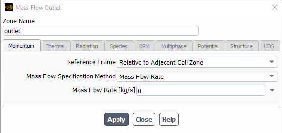
Mass-flow outlets only support the Relative to Adjacent Cell Zone specification for the Reference Frame.
You can specify the mass flow rate through the outlet zone and have Ansys Fluent convert this value to mass flux, or specify the mass flux directly. For cases where the mass flux varies across the boundary, you can specify an average mass flux. For compressible problems, you can specify that the mass flow rate is adjusted to total conditions at the outlet, thus maintaining a constant exit corrected mass flow rate.
You can define the mass flow or mass flux rate using a profile or a user-defined function (UDF). For an example of a
mass-flow outlet UDF, see DEFINE_PROFILE in the Fluent Customization Manual.
Important: The hooked UDF or transient profile can only be used to provide time-varying specification of mass flow or mass flux rate. Therefore, the transient solver must be used to run the simulation. Note that the variation of profile with position in space is not applicable with this hookup.
The inputs for mass flow rate or flux are as follows:
Make a selection in the Mass Flow Specification Method drop-down list to specify whether you will define a Mass Flow Rate, Mass Flux, Mass Flux with Average Mass Flux, or (if the density of the material is defined either as an ideal gas or using a real gas model) Exit Corrected Mass Flow Rate.
If you selected Mass Flow Rate (the default), enter the prescribed Mass Flow Rate when constant is selected from the drop-down list. Otherwise, select your hooked user-defined function (UDF) or transient profile.
If you selected Mass Flux, enter the prescribed Mass Flux (or select your hooked UDF or profile).
If you selected Mass Flux with Average Mass Flux, enter the prescribed Mass Flux (or select your hooked UDF or profile) and Average Mass Flux.
Note that if you specify a mass flux profile such that the average mass flux integrated over the zone area is 4.7, but you actually want to have a total mass flux of 5, you can keep the profile unchanged, and specify an average mass flux of 5. Ansys Fluent will maintain the profile shape but adjust the values so that the resulting mass flux across the boundary is 5.
If you selected Exit Corrected Mass Flow Rate, enter the prescribed Exit Corrected Mass Flow Rate (or select your hooked UDF or profile); this corresponds to
 in Equation 7–102. Then enter the ECMF Reference
Temperature (
in Equation 7–102. Then enter the ECMF Reference
Temperature ( ) and the ECMF Reference Gauge Pressure (
 ). For complete details about this method, see Exit Corrected Mass Flow Rate.
Important: Note that for axisymmetric problems:
If you provide a mass flow rate, you must specify the flow rate through the entire (
 -radian) domain, not through a 1-radian slice.
If you provide a mass flux rate, you must specify the flux through a 1-radian slice of the domain.
The mass flow boundary will be pumping flow out of the domain normal to the boundary at the prescribed rate or flux. If the mass flow rate is specified, then by default, the fluxes on the boundary will be allowed to vary to preserve the flow profile out of the domain. At convergence, the total mass flow rate should match the specified value.
Important: Note that if constant mass flux is needed rather than the default variable fluxes to preserve the profiles, then you can
do so via the text command define/boundary-conditions/bc-settings/mass-flow. Answer
no when asked to preserve profile while flow leaves.
The options available depend on which radiation model is active. For details, see Defining Boundary Conditions for Radiation.
If you are modeling a discrete phase of particles, you can set the fate of particle trajectories at the mass-flow outlet. See Setting Boundary Conditions for the Discrete Phase for details.
For the Mass Flow Rate specification method, you specify the total mass flow rate,  , for the outlet. For the Mass Flux or Mass Flux with Averaged Mass
Flux specification methods, you specify the mass flux,
, for the outlet. For the Mass Flux or Mass Flux with Averaged Mass
Flux specification methods, you specify the mass flux,  (mass flow rate per unit area). If a total mass flow rate is specified, Ansys Fluent converts it internally to
a uniform mass flux by dividing the mass flow rate by the total outlet area:
(mass flow rate per unit area). If a total mass flow rate is specified, Ansys Fluent converts it internally to
a uniform mass flux by dividing the mass flow rate by the total outlet area:
 | (7–101) |
If the direct mass flux specification option is used, the mass flux can be varied over the boundary by using profile files or user-defined functions. If the average mass flux is also specified, it is used to correct the specified mass flux profile, as described previously in this section.
Once the value of  at a given face has been determined, the density,
  , at the face must be determined in order to find the normal velocity,
  .
.
Boundary velocities are scaled to achieve the specified value of mass flow rate or mass flux. When the mass-flow outlet is used with the profile preserving feature, a scaling factor of the specified mass flow rate over the computed mass flow rate at the boundary is used to scale the normal face velocities at the boundary. The other velocity components will be extrapolated from the interior. Flow variables such as pressure, temperature, species, or other scalar quantities will be also extrapolated from adjacent cell centers.
The Exit Corrected Mass Flow Rate specification method adjusts the mass flow rate to the total conditions at the outlet, maintaining a constant exit corrected mass flow rate. This boundary option is mainly intended for turbomachinery applications. This method allows you to sweep through the complete machine operational range, including machine operating points from choked flow to stall conditions. When using the Exit Corrected Mass Flow Rate specification method, the boundary operates like a mass-flow outlet on the left side of the speedline curve away from the best efficiency point, and more like a pressure outlet boundary to the right of the best efficiency point all the way beyond the choke point. This method allows you to specify the equivalent mass flow, based on similar criteria, corrected to a specified reference temperature and pressure.
For compressible flows, the exit corrected mass flow rate () is calculated as:
 | (7–102) |
where  and
and  are mass-averaged values of total pressure and temperature in the absolute frame at the outlet.
and are the reference conditions, which are constants in the equation. It should be noted that the numerical
behavior of the boundary condition is not affected by the choice of reference conditions; rather, the reference conditions
simply provide a dimensional meaning to the otherwise non-dimensional mass flow rate. It is typical to specify these reference
conditions to be the same as the inflow total pressure and temperature.
are mass-averaged values of total pressure and temperature in the absolute frame at the outlet.
and are the reference conditions, which are constants in the equation. It should be noted that the numerical
behavior of the boundary condition is not affected by the choice of reference conditions; rather, the reference conditions
simply provide a dimensional meaning to the otherwise non-dimensional mass flow rate. It is typical to specify these reference
conditions to be the same as the inflow total pressure and temperature.
In order to maintain a constant exit corrected mass flow, you can observe that the resulting mass flow rate must be proportional to the exit total pressure and inversely proportional to the square root of the exit total temperature (or equivalently, inversely proportional to the stagnation speed of sound). This allows the boundary condition to adapt dynamically to varying operating conditions, while remaining stable as the flow develops from the initial guess.
Note that the Exit Corrected Mass Flow Rate specification method is only available for ideal gas and real gas materials.
You can obtain an initial exit corrected mass flow rate value () from a previously converged case that uses standard inlet and outlet boundaries (for example, a pressure
inlet and a pressure outlet). Use the converged solution to obtain the mass-flow-averaged value of and at the outlet boundary, as well as the mass flow rate ( ). These values can then be applied to Equation 7–102 along with and (which are usually taken as the inflow total temperature and pressure). After you have calculated the exit
corrected mass flow rate, you can adjust this value up or down in order to traverse the speed line from choke to stall.
). These values can then be applied to Equation 7–102 along with and (which are usually taken as the inflow total temperature and pressure). After you have calculated the exit
corrected mass flow rate, you can adjust this value up or down in order to traverse the speed line from choke to stall.
Inlet vent boundary conditions are used to model an inlet vent with a specified loss coefficient, flow direction, and ambient (inlet) pressure and temperature.
You will enter the following information for an inlet vent boundary:
type of reference frame
total (stagnation) pressure
total (stagnation) temperature
flow direction
static pressure
turbulence parameters (for turbulent calculations)
radiation parameters (for calculations using the P-1, DTRM, DO, surface-to-surface, or MC models)
chemical species mass or mole fractions (for species calculations)
mixture fraction and variance (for non-premixed or partially premixed combustion calculations)
progress variable (for premixed or partially premixed combustion calculations)
discrete phase boundary conditions (for discrete phase calculations)
multiphase boundary conditions (for general multiphase calculations)
loss coefficient
open channel flow parameters (for open channel flow calculations using the VOF multiphase model)
All values are entered in the Inlet Vent Dialog Box (Figure 7.40: The Inlet Vent Dialog Box), which is opened from the Boundary Conditions task page (as described in Setting Cell Zone and Boundary Conditions).
The first 12 items listed above are specified in the same way that they are specified at pressure inlet boundaries. See Inputs at Pressure Inlet Boundaries for details. Specification of the loss coefficient is described here. Open channel boundary condition inputs are described in Modeling Open Channel Flows.
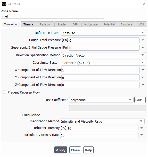
An inlet vent is considered to be infinitely thin, and the pressure drop through the vent is assumed to be proportional to
the dynamic head of the fluid, with an empirically determined loss coefficient that you supply. That is, the pressure drop,
 , varies with the normal component of velocity through the vent,
  , as follows:
 | (7–103) |
where  is the fluid density, and
  is the non-dimensional loss coefficient.
Important:  is the pressure drop in the direction of the flow; therefore the vent will appear as a resistance even
in the case of backflow.
is the pressure drop in the direction of the flow; therefore the vent will appear as a resistance even
in the case of backflow.
You can define the Loss-Coefficient across the vent as a constant, polynomial, piecewise-linear, or piecewise-polynomial function of the normal velocity. The dialog boxes for defining these functions are the same as those used for defining temperature-dependent properties. See Defining Properties Using Temperature-Dependent Functions for details.
Intake fan boundary conditions are used to model an external intake fan with a specified pressure jump, flow direction, and ambient (intake) pressure and temperature.
Note: The intake fan boundary condition considers only momentum. Diffusion processes are not considered.
You will enter the following information for an intake fan boundary:
type of reference frame
total (stagnation) pressure
total (stagnation) temperature
flow direction
static pressure
turbulence parameters (for turbulent calculations)
radiation parameters (for calculations using the P-1, DTRM, DO, surface-to-surface, or MC models)
chemical species mass or mole fractions (for species calculations)
mixture fraction and variance (for non-premixed or partially premixed combustion calculations)
progress variable (for premixed or partially premixed combustion calculations)
discrete phase boundary conditions (for discrete phase calculations)
multiphase boundary conditions (for general multiphase calculations)
pressure jump
open channel flow parameters (for open channel flow calculations using the VOF multiphase model)
All values are entered in the Intake Fan Dialog Box (shown in Figure 7.41: The Intake Fan Dialog Box), which is opened from the Boundary Conditions task page (as described in Setting Cell Zone and Boundary Conditions ).
The first 12 items listed above are specified in the same way that they are specified at pressure inlet boundaries. See Inputs at Pressure Inlet Boundaries for details. Specification of the pressure jump is described here. Open channel boundary condition inputs are described in Modeling Open Channel Flows.

An intake fan is considered to be infinitely thin, and the discontinuous pressure rise across it is specified as a function of the velocity through the fan. In the case of reversed flow, the fan is treated like an outlet vent with a loss coefficient of unity.
You can define the Pressure-Jump across the fan as a constant, polynomial, piecewise-linear, or piecewise-polynomial function of the normal velocity. The dialog boxes for defining these functions are the same as those used for defining temperature-dependent properties. See Defining Properties Using Temperature-Dependent Functions for details.
Pressure outlet boundary conditions require the specification of a static (gauge) pressure at the outlet boundary. The value of the specified static pressure is used only while the flow is subsonic. Should the flow become locally supersonic, the specified pressure will no longer be used; pressure will be extrapolated from the flow in the interior. All other flow quantities are extrapolated from the interior.
A set of “backflow” conditions is also specified should the flow reverse direction at the pressure outlet boundary during the solution process. Convergence difficulties will be minimized if you specify realistic values for the backflow quantities.
Several options in Ansys Fluent exist, where a radial equilibrium outlet boundary condition can be used (see Defining Static Pressure and a target mass flow rate for pressure outlets (see Target Mass Flow Rate Option for details) can be specified.
For an overview of flow boundaries, see Flow Inlet and Exit Boundary Conditions.
You will enter or select the following information for a pressure outlet boundary:
static pressure
pressure profile multiplier
backflow conditions
total (stagnation) temperature (for energy calculations)
backflow pressure specification
backflow direction specification method
turbulence parameters (for turbulent calculations)
chemical species mass or mole fractions (for species calculations)
mixture fraction and variance (for non-premixed or partially premixed combustion calculations)
progress variable (for premixed or partially premixed combustion calculations)
multiphase boundary conditions (for general multiphase calculations)
type of backflow reference frame (not available for multiphase flows or with the acoustic wave model)
radiation parameters (for calculations using the P-1, DTRM, DO, surface-to-surface, or MC models)
discrete phase boundary conditions (for discrete phase calculations)
open channel flow parameters (for open channel flow calculations using the VOF multiphase model)
radial equilibrium pressure distribution
average pressure specification (not available for multiphase flows)
target mass flow rate (not available for multiphase flows)
acoustic wave model settings
All values are entered in the Pressure Outlet Dialog Box (Figure 7.42: The Pressure Outlet Dialog Box), which is opened from the Boundary Conditions task page (as described in Setting Cell Zone and Boundary Conditions ). Note that open channel boundary condition inputs are described in Modeling Open Channel Flows, and acoustic wave model settings are described in Boundary Acoustic Wave Models.
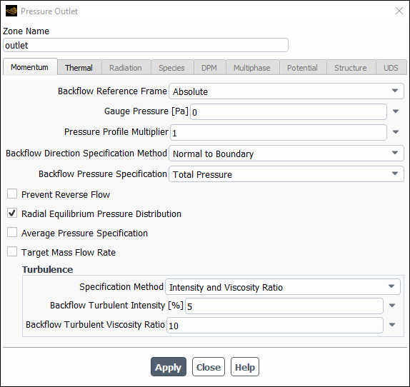
To set the static pressure at the pressure outlet boundary, enter the appropriate value for Gauge Pressure in the Pressure Outlet dialog box. This value will be used when the flow is locally subsonic. Should the flow become locally supersonic, the pressure will be extrapolated from the upstream conditions. By default the subsonic and supersonic local flow condition at the boundary is determined based on the local normal velocity component.
Remember that the static pressure value you enter is relative to the operating pressure set in the Operating Conditions Dialog Box. Refer to Pressure Inputs and Hydrostatic Head regarding hydrostatic pressure.
Ansys Fluent also provides an option to use a radial equilibrium outlet boundary condition. This option is used to model the exit flow in turbomachinery flow problems. To turn on this option, enable Radial Equilibrium Pressure Distribution. When this feature is active, the specified gauge pressure applies only to the position of minimum radius (relative to the axis of rotation) at the boundary. The static pressure on the rest of the zone is calculated from the assumption that radial velocity is negligible, so that the pressure gradient is given by
 | (7–104) |
where  is the distance from the axis of rotation and
  is the tangential velocity. Note that this boundary condition can be used even if the rotational velocity is
zero. For example, it could be applied to the calculation of the flow through an annulus containing guide vanes.
is the tangential velocity. Note that this boundary condition can be used even if the rotational velocity is
zero. For example, it could be applied to the calculation of the flow through an annulus containing guide vanes.
Important: Note that the radial equilibrium outlet condition is available only for 3D and axisymmetric swirl calculations.
Ansys Fluent also provides an option to use an Average Pressure Specification method at the pressure outlet boundary. This option allows the pressure along the outlet boundary to vary, but maintain an average equivalent to the specified value in the Gauge Pressure input field. The pressure variation allowed in this boundary implementation slightly diminishes the reflectivity of the boundary as compared with the default uniform pressure specification. In the density-based solver two averaging methods are available, Strong Averaging and Weak Averaging. The average pressure specification in the pressure-based solver is the same as the strong pressure averaging in the density-based solver. For more details, see Calculation Procedure at Pressure Outlet Boundaries.
The Pressure Profile Multiplier allows you to specify a constant factor by which the Gauge Pressure is multiplied. This is provided mainly for cases where a non-uniform distribution of the static pressure at the pressure outlet boundary is specified by means of a profile file or a user-defined function. The scaling of an outlet profile with a multiplier can be convenient, for example, when computing a performance map for a turbomachine at different mass flow rates. The option will also work for a constant Gauge Pressure simply by scaling its value by a factor. This scaled pressure value will be used consistently when additional options are enabled in the Pressure Outlet dialog box; for example, when the Radial Equilibrium Pressure Distribution option is enabled, the scaled gauge pressure will be applied to the position of minimum radius (relative to the axis of rotation) at the boundary.
Backflow properties consistent with the models you are using will appear in the Pressure Outlet dialog box. The specified values will be used only if flow is pulled in through the outlet.
The Backflow Total Temperature (in the Thermal tab) should be set for problems involving energy calculation.
When the direction of the backflow re-entering the computational domain is known, and deemed to be relevant to the flow field solution, you can specify it choosing one of the options available in the Backflow Direction Specification Method drop-down list. The default value for this field is Normal to Boundary, and requires no further input. If you choose Direction Vector, the dialog box will expand to show the inputs for the components of the direction vector for the backflow, and if you are running the 3D version of Ansys Fluent, the dialog box will display a Coordinate System drop-down list. If you choose From Neighboring Cell, Ansys Fluent will determine the direction of the backflow using the direction of the flow in the cell layer adjacent to the pressure outlet.
For turbulent calculations, there are several ways in which you can define the turbulence parameters. Instructions for deciding which method to use in determining appropriate values for these inputs are provided in Determining Turbulence Parameters. Turbulence modeling in general is described in Modeling Turbulence.
If you are modeling species transport, you will set the backflow species mass or mole fractions under Species Mass Fractions or Species Mole Fractions. For details, see Defining Cell Zone and Boundary Conditions for Species.
If you are modeling combustion using the non-premixed or partially premixed combustion model, you will set the backflow mixture fraction and variance values. See Defining Non-Premixed Boundary Conditions for details.
If you are modeling combustion using the premixed or partially premixed combustion model, you will set the backflow Progress Variable value. See Setting Boundary Conditions for the Progress Variable for details.
If you are using the VOF, mixture, or Eulerian model for multiphase flow, you will need to specify volume fractions for secondary phases and (for some models) additional parameters. See Defining Multiphase Cell Zone and Boundary Conditions for details.
If backflow occurs,
The pressure you specified as the Gauge Pressure will be used to determine the total pressure or the static pressure (based on your selection from the Backflow Pressure Specification drop-down list), so you need not specify a backflow pressure value explicitly. When Total Pressure is selected for Backflow Pressure Specification, boundary face pressure values are calculated by combining the Gauge Pressure with a dynamic contribution that is based on the velocity in the adjacent cell zone; when Static Pressure is selected for Backflow Pressure Specification, the specified Gauge Pressure value is directly imposed as the boundary face pressure.
The flow direction will be based on your selection from the Backflow Direction Specification Method drop-down list.
The total temperature, total pressure, and flow directions are in absolute or relative to the adjacent cell zone reference frames, based on the Backflow Reference Frame setting specified in the Pressure Outlet dialog box.
If the cell zone adjacent to the pressure outlet is moving (that is, if you are using a moving reference frame, multiple reference frames, mixing planes, or sliding meshes) and you are using the pressure-based solver, the velocity in the dynamic contribution to total pressure (see Equation 7–88) will be absolute or relative to the motion of the cell zone, depending on whether or not the Absolute velocity formulation is selected in the General task page. For the density-based solver, the velocity in Equation 7–88 (or the Mach number in Equation 7–89) is always in the absolute frame.
Important: Even if no backflow is expected in the converged solution, you should always set realistic values to minimize convergence difficulties in the event that backflow does occur during the calculation.
The Backflow Reference Frame option is not available for all multiphase models or non-reflecting boundary condition options.
When this option is selected, Fluent will erect artificial walls on the boundary mesh faces to prevent flow back into the domain. The artificial walls are removed when the flow is no longer entering the domain and when a favorable pressure gradient is recovered at the boundary mesh faces.
When artificial walls are created, Fluent will print a message in the console window indicating the number of faces on which artificial walls have been erected and the equivalent area percentage of the boundary it represents.
Note: This feature is not available with multiphase flow.
The options available depend on which radiation model is active. For details, see Defining Boundary Conditions for Radiation.
If you are modeling a discrete phase of particles, you can set the fate of particle trajectories at the pressure outlet. See Setting Boundary Conditions for the Discrete Phase for details.
If you are using the VOF model for multiphase flow and modeling open channel flows, you will need to specify the Free Surface Level, Bottom Level, and additional parameters. See Modeling Open Channel Flows for details.
Default settings (in SI) for pressure outlet boundary conditions are as follows:
| Gauge Pressure | 0 |
| Pressure Profile Multiplier | 1 |
| Backflow Total Temperature | 300 |
| Backflow Turbulent Intensity | 5% |
| Backflow Turbulent Viscosity Ratio | 10 |
At pressure outlets, if the flow exiting the boundary is subsonic, then Ansys Fluent uses the pressure specified in the
Pressure Outlet dialog box as the static pressure of the fluid at the outlet plane,  , and extrapolates all other conditions from the interior of the domain. However, if the flow exiting the
boundary becomes supersonic, then the face pressure values are extrapolated from the interior cell pressure.
, and extrapolates all other conditions from the interior of the domain. However, if the flow exiting the
boundary becomes supersonic, then the face pressure values are extrapolated from the interior cell pressure.
When this option is selected, the exit pressure is not kept constant over the pressure outlet boundary, but instead is allowed to vary across the boundary while maintaining an average boundary pressure close to the specified static exit pressure. This option can be used for pressure specified as a constant or as a profile (for example, in turbomachinery cases with radial, axial, or radial equilibrium pressure distributions).
There are two implementations of the Average Pressure Specification. These are Strong Averaging and Weak Averaging. The strong averaging approach is available in both the density-based and the pressure-based solver. The weak averaging approach is available only in the density-based solver.
Note:
The Average Pressure Specification option is not available with multiphase flows.
When using the density-based solver, Strong Averaging is the recommended method and is used by default. The weak averaging method is maintained primarily for legacy simulations.
When one of the Acoustic Wave Models is active, the Average Pressure Specification option is not offered because the pressure will be obtained based on the Acoustic Wave Model chosen.
Using the Average Pressure Specification option in unsteady simulations can result in nonphysical pressure feedback and is not recommended.
In the Strong Averaging approach, the face pressure value  for subsonic exit flow is computed using the following expression:
 | (7–105) |
|
where |
|
|
| |
|
| |
|
|


When the strong averaging option is used with a profile specification method (radial, axial, or radial equilibrium pressure distribution) then the outlet boundary will be subdivided into radial or axial containers called “bins”, and the above averaging procedure is applied to each bin.
You can use the following TUI command to change the blending factor and the number of bins:
/define/boundary-conditions/bc-settings/pressure-outlet
When the weak averaging method is used and the flow is subsonic, the pressure at the faces of the outlet boundary is
computed using a weighted average of the left and right state of the face boundary. This weighting is a blend of
fifth-order polynomials based on the exit face normal Mach number [91]. Therefore, the face
pressure  is a function of (
 ,
,  ,
,  ), where
  is the interior cell pressure neighboring the exit face f,
  is the specified exit pressure, and
  is the face normal Mach number.
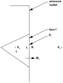
For incompressible flows, the face pressure is computed as an average between the specified pressure and the interior pressure.
 | (7–106) |
In this boundary implementation, the exit pressure is not constant along the pressure outlet boundary. However, upon flow convergence, the average boundary pressure will be close to the specified static exit pressure.
One of the options that may be used at pressure outlets is non-reflecting boundary conditions (NRBC). This option is used when waves are made to pass through the boundaries while avoiding false reflections. Details of non-reflecting boundary conditions can be found in General Non-Reflecting Boundary Conditions.
The simple Bernoulli's equation is used to adjust the pressure at every iteration on a pressure outlet zone in order to meet the desired mass flow rate. The change in pressure, based on Bernoulli’s equation is given by the following equation:
 | (7–107) |
where  is the change in pressure,
  is the current computed mass flow rate at the pressure-outlet boundary,
  is the required mass flow rate,
  is the computed average density at the pressure-outlet boundary, and
  is the area of the pressure-outlet boundary.
Limitations
The target mass flow rate option is not available with multiphase flows or when any of the non-reflecting boundary conditions models are used.
If the pressure-outlet zone is used in the mixing-plane model, the target mass flow rate option will not be available for that particular zone.
The pressure outlet will not achieve the target mass flow rate if the flow becomes choked (that is, the Mach number of the fluid in the pressure-outlet zone becomes equal to 1).
The pressure outlet may not achieve the target mass flow rate if porous zones are present in the flow domain causing a large pressure drop.
Target Mass Flow Rate Settings
To use the target mass flow rate option
Enable Target Mass Flow Rate in the Pressure Outlet dialog box.
Specify the Target Mass Flow as either a constant value or hook a UDF to set the target mass flow rate.
The settings for the target mass flow rate option can be accessed from the
target-mass-flow-rate-settingstext command:define→boundary-conditions→target-mass-flow-rate-settingsYou will be prompted to
Set the under-relaxation factor (the default setting is 0.05).
Enable the targeted mass flow rate verbosity (the default is
no). If enabled, it prints to the console window the required mass flow rate, computed mass flow rate, mean pressure, the new pressure imposed on the outlet, and the change in pressure in SI units.
In the Pressure Outlet dialog box, specify the Upper Limit of Absolute Pressure and Lower Limit of Absolute Pressure. Specifying the range of the pressure limits improves convergence in cases with a large number of outlet boundaries, which have different pressure variations on different boundaries. You can also use the
define/boundary-conditions/pressure-outlettext command to specify these limits.
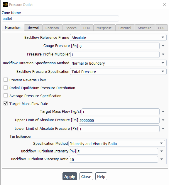
Solution Strategies When Using the Target Mass Flow Rate Option
If convergence difficulties are encountered or if the solution is not converging at the desired mass flow rate, then try to lower the under-relaxation factor from the default value. Otherwise, you can use the alternate method to converge at the required mass flow rate.
In some cases, you may want to switch off the target mass flow rate option initially, then guess an exit pressure that will bring the solution closer to the target mass flow rate. After the solution stabilizes, you can turn on the target mass flow rate option and iterate to convergence. For many complex flow problems, this strategy is usually very successful.
The use of Full Multigrid Initialization is also very helpful in obtaining a good starting solution and in general will reduce the time required to get a converged solution on a target mass flow rate. For further information on Full Multigrid Initialization, see Full Multigrid (FMG) Initialization.
Setting Target Mass Flow Rates Using UDFs
For some unsteady problems it is desirable that the target mass flow rate be a function of the physical flow time. This
enforcement of boundary condition can be done by attaching a UDF with DEFINE_PROFILE functions to the
target mass flow rate field.
Important: Note that the mass flow rate profile is a function of time and only one constant value should be applied to all zone faces at a given time.
An example of a simple UDF using a DEFINE_PROFILE that will adjust the mass flow rate can be found
in DEFINE_PROFILE in the Fluent Customization Manual.
Pressure far-field conditions are used in Ansys Fluent to model a free-stream condition at infinity, with free-stream Mach number and static conditions being specified. The pressure far-field boundary condition is often called a characteristic boundary condition, since it uses characteristic information (Riemann invariants) to determine the flow variables at the boundaries.
Note the following limitations and restrictions when using pressure far-field boundary conditions:
This boundary condition is applicable only when the density is calculated using the ideal-gas law (see Density). Using it for other flows is not permitted. To effectively approximate true infinite-extent conditions, you must place the far-field boundary far enough from the object of interest. For example, in lifting airfoil calculations, it is not uncommon for the far-field boundary to be a circle with a radius of 20 chord lengths.
It is incompatible with the multiphase models (VOF, mixture, and Eulerian) that are available with the pressure-based solver.
It cannot be applied to flows that employ constant density, the real gas model, and the wet steam model, which are available in the density-based solver.
For an overview of flow boundaries, see Flow Inlet and Exit Boundary Conditions.
You will enter the following information for a pressure far-field boundary:
static pressure
Mach number
temperature
flow direction
turbulence parameters (for turbulent calculations)
radiation parameters (for calculations using the P-1, DTRM, DO, surface-to-surface, or MC models)
chemical species mass or mole fractions (for species calculations)
discrete phase boundary conditions (for discrete phase calculations)
All values are entered in the Pressure Far-Field Dialog Box (Figure 7.45: The Pressure Far-Field Dialog Box), which is opened from the Boundary Conditions task page (as described in Setting Cell Zone and Boundary Conditions).
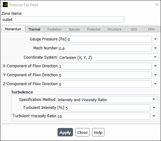
To set the static pressure and temperature at the far-field boundary in the Pressure Far-Field dialog box, enter the appropriate values for Gauge Pressure and Mach Number in the Momentum tab. The Mach number can be subsonic, sonic, or supersonic. Set the Temperature in the Thermal tab.
You can define the flow direction at a pressure far-field boundary by setting the components of the direction vector. If your geometry is 2D non-axisymmetric enter appropriate values for X and Y in the Pressure Far-Field dialog box (Figure 7.45: The Pressure Far-Field Dialog Box). If your geometry is 2D axisymmetric, enter the appropriate values for Axial, Radial, and (if you are modeling axisymmetric swirl) Tangential-Component of Flow Direction.
If your geometry is 3D, you can choose a Coordinate System that is Cartesian, Cylindrical, or Local Cylindrical. In the Cartesian coordinate system, enter the appropriate values for X, Y, and Z-Component of Flow Direction. If the direction cosine data on the boundary is available, then use the cylindrical or local cylindrical coordinate system and specify the Axial, Radial, Tangential-Component of Flow Direction. For Cylindrical, axis parameters need to be specified on the adjacent cell zone of the boundary face. For Local Cylindrical Swirl, specify the Axis Origin and Axis Direction.
For turbulent calculations, there are several ways in which you can define the turbulence parameters. Instructions for deciding which method to use and determining appropriate values for these inputs are provided in Determining Turbulence Parameters. Turbulence modeling is described in Modeling Turbulence.
The options available depend on which radiation model is active. For details, see Defining Boundary Conditions for Radiation.
If you are modeling species transport, you will set the species mass or mole fractions under Species Mass Fractions or Species Mole Fractions. See Defining Cell Zone and Boundary Conditions for Species for details.
If you are modeling a discrete phase of particles, you can set the fate of particle trajectories at the pressure far-field boundary. See Setting Boundary Conditions for the Discrete Phase for details.
Default settings (in SI) for pressure far-field boundary conditions are as follows:
| Gauge Pressure | 0 |
| Mach Number | 0.6 |
| Temperature | 300 |
| X-Component of Flow Direction | 1 |
| Y-Component of Flow Direction | 0 |
| Z-Component of Flow Direction | 0 |
| Turbulent Intensity | 5% |
| Turbulent Viscosity Ratio | 10 |
The pressure far-field boundary condition is a non-reflecting boundary condition based on the introduction of Riemann invariants (that is, characteristic variables) for a one-dimensional flow normal to the boundary. For flow that is subsonic there are two Riemann invariants, corresponding to incoming and outgoing waves:
 | (7–108) |
 | (7–109) |
where  is the velocity magnitude normal to the boundary,
  is the local speed of sound and
  is the ratio of specific heats (ideal gas). The subscript
  refers to conditions being applied at infinity (the boundary conditions), and the subscript
  refers to conditions in the interior of the domain (that is, in the cell adjacent to the boundary face). These
two invariants can be added and subtracted to give the following two equations:
refers to conditions in the interior of the domain (that is, in the cell adjacent to the boundary face). These
two invariants can be added and subtracted to give the following two equations:
 | (7–110) |
 | (7–111) |
where  and
and  become the values of normal velocity and sound speed applied on the boundary. At a face through which flow
exits, the tangential velocity components and entropy are extrapolated from the interior; at an inflow face, these are specified
as having free-stream values. Using the values for
become the values of normal velocity and sound speed applied on the boundary. At a face through which flow
exits, the tangential velocity components and entropy are extrapolated from the interior; at an inflow face, these are specified
as having free-stream values. Using the values for  ,
,  , tangential velocity components, and entropy the values of density, velocity, temperature, and pressure at the
boundary face can be calculated.
, tangential velocity components, and entropy the values of density, velocity, temperature, and pressure at the
boundary face can be calculated.
Fluent’s density-based solver offers an alternative method for the pressure far-field boundary condition. This method employs a Riemann solver to evaluate the numerical flux at the far-field boundary, thus providing the same level of accuracy and robustness as the interior faces. This treatment is a global application of the local tangency-correction used to regain robustness on boundary faces tangent to the imposed flow direction (as described in Tangency Correction). It is also advantageous for calculations where boundary layers or wakes extend beyond the boundary of the computational domain. This flux-based pressure far-field can be selected with the following text command:
/define/boundary-condition/bc-settings/pressure-far-field/type?
Depending on the choice of computational domain, certain boundary-faces might be tangent to the imposed free-stream flow direction. Flow tangency along a pressure far-field boundary hinders the solver robustness. To regain robustness in such situations, a local tangency-correction has been implemented in Fluent’s density-based solver. This correction locally replaces the standard Riemann-invariants boundary treatment by a numerical-flux evaluation, analogous to using a Riemann solver. The correction is active by default, and can be deactivated with the following text command:
/define/boundary-condition/bc-settings/pressure-far-field/riemann-invariants-tangency-correction?
Outflow boundary conditions in Ansys Fluent are used to model flow exits where the details of the flow velocity and pressure are not known prior to solving the flow problem. You do not define any conditions at outflow boundaries (unless you are modeling radiative heat transfer, a discrete phase of particles, or split mass flow): Ansys Fluent extrapolates the required information from the interior. It is important, however, to understand the limitations of this boundary type.
Important: Note that outflow boundaries cannot be used in the following cases:
If a problem includes pressure inlet boundaries; use pressure outlet boundary conditions (see Pressure Outlet Boundary Conditions) instead.
If you are modeling compressible flow.
If you are modeling unsteady flows with varying density (even if the fluid is incompressible), it is preferable to use a pressure outlet.
In general, an outflow condition may be used in incompressible cases using the Eulerian or Mixture multiphase models. However, if the flow may produce a recirculation at the outlet or if the flow field is not stable and fully developed at the outlet, then a pressure outlet boundary condition is preferred.
For an overview of flow boundaries, see Flow Inlet and Exit Boundary Conditions.
The boundary conditions used by Ansys Fluent at outflow boundaries are as follows:
A zero diffusion flux for all flow variables.
An overall mass balance correction.
The zero diffusion flux condition applied at outflow cells means that the conditions of the outflow plane are extrapolated from within the domain and have no impact on the upstream flow. The extrapolation procedure used by Ansys Fluent updates the outflow velocity and pressure in a manner that is consistent with a fully-developed flow assumption, as noted below, when there is no area change at the outflow boundary.
The zero diffusion flux condition applied by Ansys Fluent at outflow boundaries is approached physically in fully-developed flows. Fully-developed flows are flows in which the flow velocity profile (and/or profiles of other properties such as temperature) is unchanging in the flow direction.
It is important to note that gradients in the cross-stream direction may exist at an outflow boundary. Only the diffusion fluxes in the direction normal to the exit plane are assumed to be zero.
As noted in Ansys Fluent’s Treatment at Outflow Boundaries, the outflow boundary condition is obeyed in fully-developed flows where the diffusion flux for all flow variables in the exit direction are zero. However, you may also define outflow boundaries at physical boundaries where the flow is not fully developed—and you can do so with confidence if the assumption of a zero diffusion flux at the exit is expected to have a small impact on your flow solution. The appropriate placement of an outflow boundary is described by example below.
Outflow boundaries where normal gradients are negligible: Figure 7.46: Choice of the Outflow Boundary Condition Location shows a simple two-dimensional flow problem and several possible outflow boundary location choices. Location C shows the outflow boundary located upstream of the plenum exit but in a region of the duct where the flow is fully-developed. At this location, the outflow boundary condition is exactly obeyed.
Ill-posed outflow boundaries: Location B in Figure 7.46: Choice of the Outflow Boundary Condition Location shows the outflow boundary near the reattachment point of the recirculation in the wake of the backward-facing step. This choice of outflow boundary condition is ill-posed as the gradients normal to the exit plane are quite large at this point and can be expected to have a significant impact on the flow field upstream. Because the outflow boundary condition ignores these axial gradients in the flow, location B is a poor choice for an outflow boundary. The exit location should be moved downstream from the reattachment point.
Figure 7.46: Choice of the Outflow Boundary Condition Location shows a second ill-posed outflow boundary at location A. Here, the outflow is located where flow is pulled into the Ansys Fluent domain through the outflow boundary. In situations like this the Ansys Fluent calculation typically does not converge and the results of the calculation have no validity. This is because when flow is pulled into the domain through an outflow, the mass flow rate through the domain is “floating” or undefined. In addition, when flow enters the domain through an outflow boundary, the scalar properties of the flow are not defined. For example, the temperature of the flow pulled in through the outflow is not defined. (Ansys Fluent chooses the temperature using the temperature of the fluid adjacent to the outflow, inside the domain.) Therefore you should view all calculations that involve flow entering the domain through an outflow boundary with skepticism. For such calculations, pressure outlet boundary conditions (see Pressure Outlet Boundary Conditions) are recommended.
Important: Note that convergence may be affected if there is recirculation through the outflow boundary at any point during the calculation, even if the final solution is not expected to have any flow reentering the domain. This is particularly true of turbulent flow simulations.
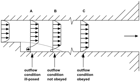
In Ansys Fluent, it is possible to use multiple outflow boundaries and specify the fractional flow rate through each boundary. In the Outflow Dialog Box, set the Flow Rate Weighting to indicate what portion of the outflow is through the boundary.
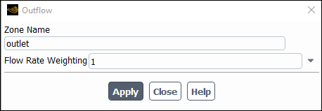
The Flow Rate Weighting is a weighting factor:
 | (7–112) |
By default, the Flow Rate Weighting for all outflow boundaries is set to 1. If the flow is divided equally among all of your outflow boundaries (or if you have just one outflow boundary), you need not change the settings from the default; Ansys Fluent will scale the flow rate fractions to obtain equal fractions through all outflow boundaries. Therefore, if you have two outflow boundaries and you want half of the flow to exit through each one, no inputs are required from you. If, however, you want 75% of the flow to exit through one, and 25% through the other, you will need to explicitly specify both Flow Rate Weighting values, that is, 0.75 for one boundary and 0.25 for the other.
Important: If you specify a Flow Rate Weighting of 0.75 at the first exit and leave the default Flow Rate Weighting (1.0) at the second exit, then the flow through each boundary will be
Boundary 1 =  = 0.429 or 42.9% = 0.429 or 42.9% |
Boundary 2 =  = 0.571 or 57.1% = 0.571 or 57.1% |
In general, there are no boundary conditions for you to set at an outflow boundary. If, however, you are using the P-1, DTRM, DO, surface-to-surface, or MC models, you will set the Internal Emissivity and (optionally) External Black Body Temperature Method in the Outflow dialog box. These parameters are described in Defining Boundary Conditions for Radiation. The default value for Internal Emissivity is 1 and the default value for Black Body Temperature is 300.
If you are modeling a discrete phase of particles, you can set the fate of particle trajectories at the outflow boundary. See Setting Boundary Conditions for the Discrete Phase for details.
Outlet vent boundary conditions are used to model an outlet vent with a specified loss coefficient and ambient (discharge) pressure and temperature.
You will enter the following information for an outlet vent boundary:
static pressure
backflow conditions
total (stagnation) temperature (for energy calculations)
backflow pressure specification
backflow direction specification method
turbulence parameters (for turbulent calculations)
chemical species mass or mole fractions (for species calculations)
mixture fraction and variance (for non-premixed or partially premixed combustion calculations)
progress variable (for premixed or partially premixed combustion calculations)
multiphase boundary conditions (for general multiphase calculations)
type of backflow reference frame (not available for multiphase flows)
radiation parameters (for calculations using the P-1, DTRM, DO, surface-to-surface, or MC models)
discrete phase boundary conditions (for discrete phase calculations)
loss coefficient
open channel flow parameters (for open channel flow calculations using the VOF multiphase model)
All values are entered in the Outlet Vent Dialog Box (Figure 7.48: The Outlet Vent Dialog Box), which is opened from the Boundary Conditions task page (as described in Setting Cell Zone and Boundary Conditions).
The first 4 items listed above are specified in the same way that they are specified at pressure outlet boundaries. See Inputs at Pressure Outlet Boundaries for details. Specification of the loss coefficient is described here. Open channel boundary condition inputs are described in Modeling Open Channel Flows.
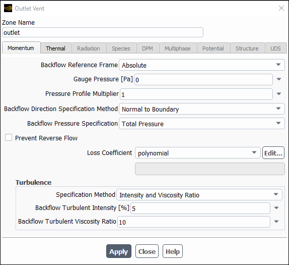
An outlet vent is considered to be infinitely thin, and the pressure drop through the vent is assumed to be proportional to
the dynamic head of the fluid, with an empirically determined loss coefficient that you supply. That is, the pressure drop,
 , varies with the normal component of velocity through the vent,
  , as follows:
 | (7–113) |
where  is the fluid density, and
  is the nondimensional loss coefficient.
Important:  is the pressure drop in the direction of the flow; therefore the vent will appear as a resistance even
in the case of backflow.
is the pressure drop in the direction of the flow; therefore the vent will appear as a resistance even
in the case of backflow.
You can define a constant, polynomial, piecewise-linear, or piecewise-polynomial function for the Loss Coefficient across the vent. The dialog boxes for defining these functions are the same as those used for defining temperature-dependent properties. See Defining Properties Using Temperature-Dependent Functions for details.
Exhaust fan boundary conditions are used to model an external exhaust fan with a specified pressure jump and ambient (discharge) pressure.
Note: The exhaust fan boundary condition considers only momentum. Diffusion processes are not considered.
You will enter the following information for an exhaust fan boundary:
static pressure
backflow conditions
total (stagnation) temperature (for energy calculations)
backflow pressure specification
backflow direction specification method
turbulence parameters (for turbulent calculations)
chemical species mass or mole fractions (for species calculations)
mixture fraction and variance (for non-premixed or partially premixed combustion calculations)
progress variable (for premixed or partially premixed combustion calculations)
multiphase boundary conditions (for general multiphase calculations)
type of backflow reference frame (not available for multiphase flows)
user-defined scalar boundary conditions (for user-defined scalar calculations)
radiation parameters (for calculations using the P-1, DTRM, DO, surface-to-surface, or MC models)
discrete phase boundary conditions (for discrete phase calculations)
pressure jump
open channel flow parameters (for open channel flow calculations using the VOF multiphase model)
All values are entered in the Exhaust Fan Dialog Box (Figure 7.49: The Exhaust Fan Dialog Box), which is opened from the Boundary Conditions task page (as described in Setting Cell Zone and Boundary Conditions).
The first 4 items listed above are specified in the same way that they are specified at pressure outlet boundaries. See Inputs at Pressure Outlet Boundaries for details. Specification of the pressure jump is described here. Open channel boundary condition inputs are described in Modeling Open Channel Flows.
An exhaust fan is considered to be infinitely thin, and the discontinuous pressure rise across it is specified as a function of the local fluid velocity normal to the fan. You can define a constant, polynomial, piecewise-linear, or piecewise-polynomial function for the Pressure Jump across the fan. The dialog boxes for defining these functions are the same as those used for defining temperature-dependent properties. See Defining Properties Using Temperature-Dependent Functions for details.

Important: You must be careful to model the exhaust fan so that a pressure rise occurs for forward flow through the fan. In the case of reversed flow, the fan is treated like an inlet vent with a loss coefficient of unity.
Degassing boundary conditions are used to model a free surface through which dispersed gas bubbles are allowed to escape, but the continuous phase is not. A typical application is a bubble column in which you want to reduce computational cost by not including the freeboard region in the simulation.
When the degassing boundary condition is specified for an outlet, the continuous liquid phase sees the boundary as a free-slip wall and does not leave the domain. The dispersed gas phase sees the boundary as an outlet. The outlet pressure is not specified. Instead, Ansys Fluent automatically specifies a mass sink for the dispersed gas phase in the cells adjacent to the degassing outlet. The mass sink is calculated using the flux normal to the boundary at the cell center.
Note: The degassing boundary condition is only available for two-phase liquid-gas flows using the Eulerian multiphase model.
The following limitations apply to the degassing boundary condition in Ansys Fluent:
The degassing boundary condition is only available for liquid-gas two-phase flow using the Eulerian model. The primary phase must be liquid.
In order for the gas to escape from the degassing boundary, gravity must be switched on in the model.
The degassing boundary condition is only recommended for modeling situations like bubble columns without the freeboard region.
When postprocessing on a degassing boundary, there is no normal velocity for either phase since the gas escape is modeled by a mass sink in the neighboring cells.
No inputs are necessary for the degassing boundary condition. However, the initial condition for volume fraction must be set appropriately. It is recommended that the gas phase volume fraction be initialized with a nonzero value smaller than the steady-state gas holdup value.
Wall boundary conditions are used to bound fluid and solid regions. In viscous flows, the no-slip boundary condition is enforced at walls by default, but you can specify a tangential velocity component in terms of the translational or rotational motion of the wall boundary, or model a “slip” wall by specifying shear. (You can also model a slip wall with zero shear using the symmetry boundary type, but using a symmetry boundary will apply symmetry conditions for all equations. See Symmetry Boundary Conditions for details.)
The shear stress and heat transfer between the fluid and wall are computed based on the flow details in the local flow field.
The following topics are discussed in this section:
- 7.4.15.1. Inputs at Wall Boundaries
- 7.4.15.2. Stationary Wall
- 7.4.15.3. Wall Roughness Effects in Turbulent Wall-Bounded Flows
- 7.4.15.4. Wall Motion
- 7.4.15.5. Thermal Boundary Conditions at Walls
- 7.4.15.6. Species Boundary Conditions for Walls
- 7.4.15.7. Radiation Boundary Conditions for Walls
- 7.4.15.8. Discrete Phase Model (DPM) Boundary Conditions for Walls
- 7.4.15.9. User-Defined Scalar (UDS) Boundary Conditions for Walls
- 7.4.15.10. Wall Film Conditions for Walls
- 7.4.15.11. Structural Model Conditions for Walls
- 7.4.15.12. Default Settings at Wall Boundaries
- 7.4.15.13. Shear-Stress Calculation Procedure at Wall Boundaries
- 7.4.15.14. Heat Transfer Calculations at Wall Boundaries
You will enter the following information for a wall boundary:
wall roughness (for turbulent flows, optional)
wall motion conditions (for moving or rotating walls)
shear conditions (for slip walls, optional)
thermal boundary conditions (for heat transfer calculations)
species boundary conditions (for species calculations)
chemical reaction boundary conditions (for surface reactions)
radiation boundary conditions (for calculations using the P-1, DTRM, DO, surface-to-surface, or MC models)
discrete phase boundary conditions (for discrete phase calculations)
wall adhesion contact angle (for VOF calculations, optional)
displacement boundary conditions for intrinsic fluid-structure interaction (FSI) simulations
For a stationary wall, choose the Stationary Wall option under Wall Motion.
Fluids flows over rough surfaces are encountered in diverse situations. Examples are, among many others, flows over the surfaces of airplanes (especially due to ice accretion), ships, turbomachinery, heat exchangers, piping systems, and atmospheric boundary layers over terrain of varying roughness. Wall roughness affects drag (resistance) as well as heat and mass transfer on the walls.
If you are modeling turbulent wall-bounded flow in which the wall roughness effects are considered to be significant, you can include the wall roughness effects through the Standard Law-of-the-Wall Modified for Roughness (for details, see Wall Roughness Effects in Turbulent Wall-Bounded Flows in the Fluent Theory Guide) or you can use one of the Additional Roughness Models for Icing Simulations (for Spalart-Allmaras or the SST k-ω models only).
Note: Rough walls cannot be used together with the following model combinations:
An ϵ-equation model with enhanced wall treatment or the Menter-Lechner near-wall treatment.
Note that the following are the relevant ϵ-equations:
all of the k-ϵ models (that is, standard, RNG, and realizable).
the Reynolds stress model with Linear Pressure-Strain model selected.
the detached eddy simulation (DES) with the Realizable k-epsilon option selected.
the Reynolds stress model with the Stress-Omega or Stress-BSL model selected.
the transition k-kl-ω model.
the Large Eddy Simulation (LES) model with Kader Blending Wall Functions and Werner Wengle Wall Treatment.
The roughness parameters are in the Momentum tab of the Wall Dialog Box (see Figure 7.54: The Wall Dialog Box for Marangoni Stress), which is opened from the Boundary Conditions Task Page (as described in Setting Cell Zone and Boundary Conditions).
To model the wall roughness effects, you must specify two roughness
parameters: the Roughness Height,  , and the Roughness Constant,
 . The default roughness height (
 ) is zero, which corresponds to smooth walls. For the roughness
to take effect, you must specify a nonzero value for
) is zero, which corresponds to smooth walls. For the roughness
to take effect, you must specify a nonzero value for  . For a uniform sand-grain roughness, the height of the
sand-grain can simply be taken for
. For a uniform sand-grain roughness, the height of the
sand-grain can simply be taken for  . For a non-uniform sand-grain, however, the mean diameter
(
. For a non-uniform sand-grain, however, the mean diameter
( ) would be a more meaningful roughness height. For other types
of roughness, an “equivalent” sand-grain roughness height could be
used for
) would be a more meaningful roughness height. For other types
of roughness, an “equivalent” sand-grain roughness height could be
used for  . The above approaches are only relevant if the height is
considered constant per surface. However, if the roughness constant or roughness
height is not constant, then you can specify a profile (see Profiles). Similarly, user-defined functions may be
used to define a wall roughness height that is not constant. For details on the
format of user-defined functions, refer to the Fluent Customization Manual.
. The above approaches are only relevant if the height is
considered constant per surface. However, if the roughness constant or roughness
height is not constant, then you can specify a profile (see Profiles). Similarly, user-defined functions may be
used to define a wall roughness height that is not constant. For details on the
format of user-defined functions, refer to the Fluent Customization Manual.
Choosing a proper roughness constant ( ) is dictated mainly by the type of the given roughness. The
default roughness constant (
) is dictated mainly by the type of the given roughness. The
default roughness constant ( ) was determined so that, when used with
  -
-  turbulence models, it reproduces Nikuradse’s resistance
data for pipes roughened with tightly-packed, uniform sand-grain roughness. You
may need to adjust the roughness constant when the roughness you want to model
departs much from uniform sand-grain. For instance, there is some experimental
evidence that, for non-uniform sand-grains, ribs, and wire-mesh roughness, a
higher value (
turbulence models, it reproduces Nikuradse’s resistance
data for pipes roughened with tightly-packed, uniform sand-grain roughness. You
may need to adjust the roughness constant when the roughness you want to model
departs much from uniform sand-grain. For instance, there is some experimental
evidence that, for non-uniform sand-grains, ribs, and wire-mesh roughness, a
higher value ( ) is more appropriate. Unfortunately, a clear guideline for
choosing
) is more appropriate. Unfortunately, a clear guideline for
choosing  for arbitrary types of roughness is not available.
Additional roughness models are available if you have selected the Spalart-Allmaras or the SST k-ω model in the Viscous Model dialog box. See the Steps in Using a Turbulence Model for more information. With one of these viscous models active, the additional roughness models will be available on the Wall boundary condition panel on the Momentum tab under Wall Roughness → Roughness Models → High Roughness (Icing). A discussion of the treatment of the turbulence models with the High Roughness (Icing) enabled is given in Treatment of the Spalart-Allmaras Model for Icing Simulations and Treatment of the SST Model for Icing Simulations. These models are primarily designed and tested for simulations of icing applications, however they may also be useful for other applications in which the boundary layer is fully resolved and there is surface roughness that is large relative to the near-wall mesh.
Note that the High Roughness (Icing) models are only valid for low-Re number turbulence, or need fine near-wall meshes (mesh should fully resolve the boundary layer).
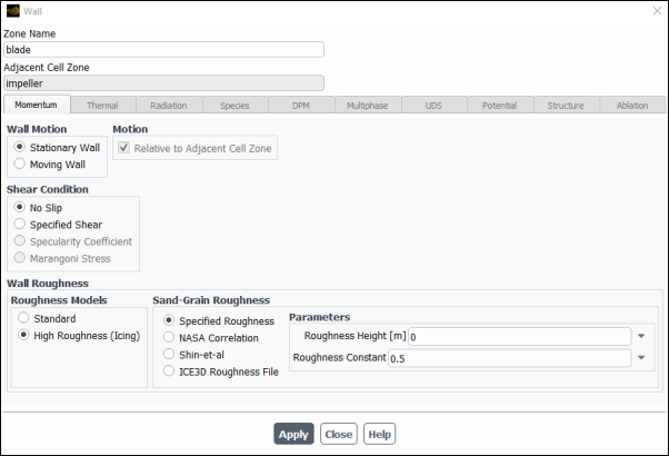
You have the following options:
Specified Roughness
NASA Correlation
Shin-et-al
ICE3D Roughness File
A Specified Roughness can be applied in the same manner as described in the section on the Standard Roughness model. See Setting the Roughness Parameters for more details.
If the NASA Correlation option is selected, the surface sand-grain roughness height is computed with an empirical NASA correlation for icing in air flows [141]. The sand-grain roughness height is computed from the product of the following coefficients:
 | (7–114) |
 | (7–115) |
 | (7–116) |
Where  is the Free Stream Velocity,
 is the Free Stream Temperature, LC is
the Liquid Content (in most cases water for ice
accretion), c is the Characteristic Length, and
is the Free Stream Temperature, LC is
the Liquid Content (in most cases water for ice
accretion), c is the Characteristic Length, and
 .
.
The sand-grain roughness height is then obtained from the formulation:
 | (7–117) |
If the Shin-et-al option is selected the empirical correlation for the surface sand-grain roughness is computed with the Shin and Bond formulation [141], which modifies the NASA correlation (see the NASA Correlation for a description of variables) with the following factor:
 | (7–118) |
where MVD is the droplet mean diameter (Droplet Diameter). The corresponding value of the sand-grain roughness height is obtained from:
 | (7–119) |
If the ICE3D Roughness File is selected, the
sand-grain roughness height is read from a node-based input file obtained
from FENSAP-ICE. The file must have the format  , and be read in Fluent via File
→ Read → Profile.
After the FENSAP-ICE roughness file is read into Fluent, the file name will
appear in the dropdown list.
, and be read in Fluent via File
→ Read → Profile.
After the FENSAP-ICE roughness file is read into Fluent, the file name will
appear in the dropdown list.
Wall boundaries can be either stationary or moving. The stationary boundary condition specifies a fixed wall, whereas the moving boundary condition can be used to specify the translational or rotational velocity of the wall, or the velocity components.
Wall motion conditions are entered in the Momentum tab of the Wall Dialog Box (Figure 7.51: The Wall Dialog Box for a Moving Wall), which is opened from the Boundary Conditions Task Page (as described in Setting Cell Zone and Boundary Conditions). To view the wall motion conditions, click the Momentum tab.
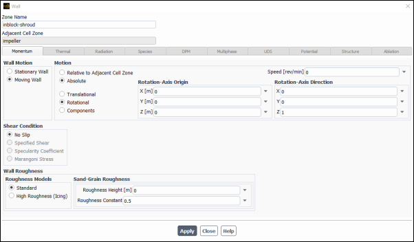
If you want to include tangential motion of the wall in your calculation, you need to define the translational or rotational velocity, or the velocity components. Select the Moving Wall option under Wall Motion. The Wall dialog box will expand, as shown in Figure 7.51: The Wall Dialog Box for a Moving Wall, to show the wall velocity conditions.
Note that you cannot use the moving wall condition to model problems where the wall motion with respect to the adjacent cell zone has a component that is normal to the wall itself. For such problems, consider using a Sliding or Dynamic Mesh approach as discussed in Modeling Flows Using Sliding and Dynamic Meshes. Ansys Fluent will neglect any normal component of wall motion that you specify using the methods below.
Specifying Relative or Absolute Velocity
If the cell zone adjacent to the wall is moving (for example, if you are using a moving reference frame or a sliding mesh), you can choose to specify velocities relative to the zone motion by enabling the Relative to Adjacent Cell Zone option. If you choose to specify relative velocities, a velocity of zero means that the wall is stationary in the relative frame, and therefore moving at the speed of the adjacent cell zone in the absolute frame. If you choose to specify absolute velocities (by enabling the Absolute option), a velocity of zero means that the wall is stationary in the absolute frame, and therefore moving at the speed of the adjacent cell zone—but in the opposite direction—in the relative reference frame.
Important: If you are using one or more moving reference frames, sliding meshes, or mixing planes, and you want the wall to be fixed in the moving frame, it is recommended that you specify relative velocities (the default) rather than absolute velocities. Then, if you modify the speed of the adjacent cell zone, you will not need to make any changes to the wall velocities, as you would if you specified absolute velocities.
Note that if the adjacent cell zone is not moving, the absolute and relative options are equivalent.
Translational Wall Motion
For problems that include linear translational motion of the wall boundary (for example, a rectangular duct with a moving belt as one wall) you can enable the Translational option and specify the wall’s Speed and Direction (X,Y,Z vector). By default, wall motion is “disabled” by the specification of Translational velocity with a Speed of zero. You can define time-varying translational speed using a transient profile (Standard Transient Profiles) or user-defined function for the speed of the wall.
If you need to define nonlinear translational motion, you will need to use the Components option, described below.
Rotational Wall Motion
For problems that include rotational wall motion you can enable the Rotational option and define the rotational Speed about a specified axis. To define the axis, set the Rotation-Axis Direction and Rotation-Axis Origin. This axis is independent of the axis of rotation used by the adjacent cell zone, and independent of any other wall rotation axis. For 3D problems, the axis of rotation is the vector passing through the specified Rotation-Axis Origin and parallel to the vector from (0,0,0) to the (X,Y,Z) point specified under Rotation-Axis Direction. For 2D problems, you will specify only the Rotation-Axis Origin; the axis of rotation is the
 -direction vector passing through the specified point. For 2D axisymmetric problems, you will not
define the axis: the rotation will always be about the
-direction vector passing through the specified point. For 2D axisymmetric problems, you will not
define the axis: the rotation will always be about the  axis, with the origin at (0,0). You can define time-varying rotational speed using a transient
profile (Standard Transient Profiles) profile or a user-defined function for the speed of the wall.
axis, with the origin at (0,0). You can define time-varying rotational speed using a transient
profile (Standard Transient Profiles) profile or a user-defined function for the speed of the wall.Note that the modeling of tangential rotational motion will be correct only if the wall bounds a surface of revolution about the prescribed axis of rotation (for example, a circle or cylinder). Note also that rotational motion can be specified for a wall in a stationary reference frame.
Wall Motion Based on Velocity Components
For problems that include linear or nonlinear translational motion of the wall boundary you can enable the Components option and specify the X-Velocity, Y-Velocity, and Z-Velocity of the wall. You can define nonlinear translational motion using a profile or a user-defined function for the X-Velocity, Y-Velocity, and/or Z-Velocity of the wall.
Wall Motion for Two-Sided Walls
As discussed earlier in this section, when you read a mesh with a two-sided wall zone (which forms the interface between fluid/solid regions) into Ansys Fluent, a “shadow” zone will automatically be created so that each side of the wall is a distinct wall zone. For two-sided walls, it is possible to specify different motions for the wall and shadow zones, whether or not they are coupled. Note, however, that you cannot specify motion for a wall (or shadow) that is adjacent to a solid zone.
Four types of shear conditions are available:
no-slip
specified shear
specularity coefficient
Marangoni stress
The no-slip condition is the default, and it indicates that the fluid sticks to the wall and moves with the same velocity as
the wall, if it is moving. The specified shear and Marangoni stress boundary conditions are useful in modeling situations in
which the shear stress (rather than the motion of the fluid) is known. Examples of such situations are applied shear stress,
slip wall (zero shear stress), and free surface conditions (zero shear stress or shear stress dependent on surface tension
gradient). The specified shear boundary condition allows you to specify the  ,
,  , and
, and  components of the shear stress as constant values or profiles. The Marangoni stress boundary condition
allows you to specify the gradient of the surface tension with respect to the temperature at this surface. The shear stress is
calculated based on the surface gradient of the temperature and the specified surface tension gradient. The Marangoni stress
option is available only for calculations in which the energy equation is being solved.
components of the shear stress as constant values or profiles. The Marangoni stress boundary condition
allows you to specify the gradient of the surface tension with respect to the temperature at this surface. The shear stress is
calculated based on the surface gradient of the temperature and the specified surface tension gradient. The Marangoni stress
option is available only for calculations in which the energy equation is being solved.
The specularity coefficient shear condition is specifically used in multiphase with granular flows. The specularity coefficient is a measure of the fraction of collisions that transfer momentum to the wall and its value ranges between zero and unity. This implementation is based on the Johnson and Jackson [74] boundary conditions for granular flows.
Shear conditions are entered in the Momentum tab of the Wall Dialog Box, which is opened from the Boundary Conditions Task Page (as described in Setting Cell Zone and Boundary Conditions ).
You can model a no-slip wall by selecting the No Slip option under Shear Condition. This is the default for all walls in viscous flows.
In addition to the no-slip wall that is the default for viscous flows, you can model a slip wall by specifying zero or
nonzero shear. For nonzero shear, the shear to be specified is the shear at the wall by the fluid. To specify the shear,
select the Specified Shear option under Shear Condition (see Figure 7.52: The Wall Dialog Box for Specified Shear). You can then enter  ,
,  , and
, and  components of shear under Shear Stress.
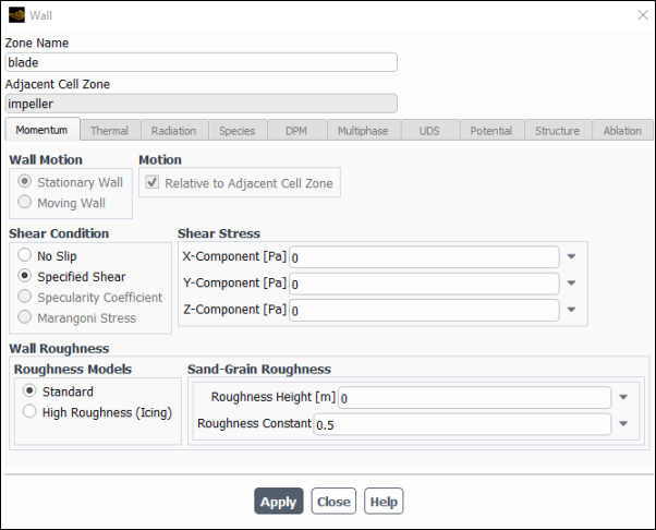
For multiphase granular flow, you can specify the specularity coefficient such that when the value is zero, this condition is equivalent to zero shear at the wall, but when the value is near unity, there is a significant amount of lateral momentum transfer. To specify the specularity coefficient, select the Specularity Coefficient option under Shear Condition (see Figure 7.53: The Wall Dialog Box for the Specularity Coefficient) and enter the desired value in the text-entry box under Specularity Coefficient.
Note: The specularity coefficient is not available for moving walls.
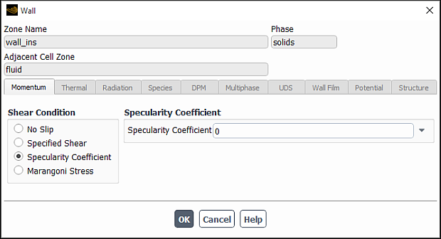
Ansys Fluent can also model shear stresses caused by the variation of surface tension due to temperature. The shear stress applied at the wall is given by
 | (7–120) |
where  is the surface tension gradient with respect to temperature, and
  is the surface gradient. This shear stress is then applied to the momentum equation.
To model Marangoni stress for the wall, select the Marangoni Stress option under Shear
Condition (see Figure 7.54: The Wall Dialog Box for Marangoni Stress). This option is available only for calculations in
which the energy equation is being solved. You can then enter the surface tension gradient ( in Equation 7–120) in the Surface Tension Gradient
field. Wall functions for turbulence are not used with the Marangoni Stress option.
in Equation 7–120) in the Surface Tension Gradient
field. Wall functions for turbulence are not used with the Marangoni Stress option.
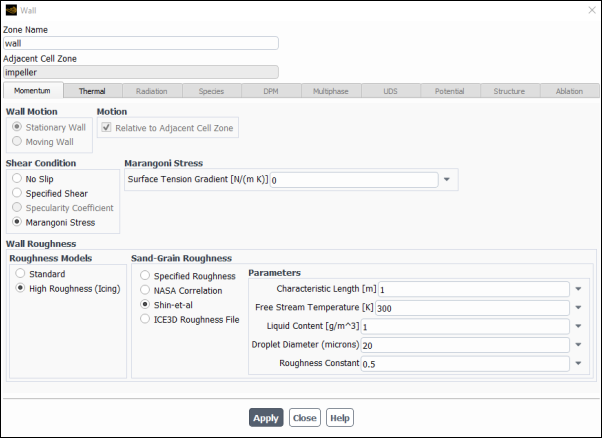
Ansys Fluent offers a partial-slip boundary condition for rarefied gases. In the rarefied regime, the finite amount of friction is no longer sufficient to allow the full adhesion of gas particles onto solid walls, see Partial Slip for Rarefied Gases.
When you are solving the energy equation, you need to define thermal boundary conditions at wall boundaries. Seven types of thermal conditions are available:
fixed heat flux
fixed temperature
convective heat transfer
external radiation heat transfer
combined external radiation and convection heat transfer
thermal data transferred between another system in Workbench using System Coupling
thermal coupling across a mapped interface
If the wall zone is a “two-sided wall” (a wall that forms the interface between two regions, such as the fluid/solid interface for a conjugate heat transfer problem) a subset of these thermal conditions will be available, but you will also be able to choose whether or not the two sides of the wall are “coupled”. See below for details.
The inputs for each type of thermal condition are described below. If the wall has a nonzero-thickness, you should also set parameters for calculating thin-wall thermal resistance and heat generation in the wall, as described below.
For a boundary wall that is adjacent to a solid cell zone that undergoes solid motion, you can model the advection of heat into or out of the domain as a result of the motion that is normal to the boundary. Details are provided in a section that follows.
You can model conduction within boundary walls and internal (that is, two-sided) walls of your model. This type of conduction, called shell conduction, allows you to more conveniently model heat conduction on walls where the wall thickness is small with respect to the overall geometry (for example, finned heat exchangers or sheet metal in automobile underhoods). Meshing these walls with solid cells would lead to high-aspect-ratio meshes and a significant increase in the total number of cells. See below for details about shell conduction.
Thermal conditions are entered in the Thermal tab of the Wall Dialog Box (Figure 7.55: The Wall Dialog Box (Thermal Tab)), which is opened from the Boundary Conditions task page (as described in Setting Cell Zone and Boundary Conditions).
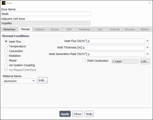
For a fixed heat flux condition, choose the Heat Flux option under Thermal Conditions. You will then need to set the appropriate value for the heat flux at the wall surface in the Heat Flux field. You can define an adiabatic wall by setting a zero heat flux condition. This is the default condition for all walls.
To select the fixed temperature condition, choose the Temperature option under Thermal Conditions in the Wall dialog box. You will need to specify the temperature at the wall surface (Temperature). The heat transfer to the wall is computed using Equation 7–123 or Equation 7–124.
For a convective heat transfer wall boundary, select Convection under Thermal Conditions. Your inputs of Heat Transfer Coefficient and Free Stream Temperature will allow Ansys Fluent to compute the heat transfer to the wall using Equation 7–127.
If radiation heat transfer from the exterior of your model is of interest, you can enable the Radiation option in the Wall dialog box and set the External Emissivity and External Radiation Temperature.
You can choose a thermal condition that combines the convection and radiation boundary conditions by selecting the Mixed option. With this thermal condition, you will need to set the Heat Transfer Coefficient, Free Stream Temperature, External Emissivity, and External Radiation Temperature.
When modeling the heat transfer of applications that have perturbed flow and/or disturbed boundary layers, it can be necessary to augment the calculation of the diffusive heat flux with a convective augmentation factor. Such applications include the modeling of underhood and underbody heat loads, as wells as transient heat transfer in fully warmed-up exhaust systems.
The convective augmentation factor represents the ratio of the measured Nusselt number to the Nusselt number of an ideal flow. You can define it by using the following text command:
define →
boundary-conditions →
wall
You will be prompted to define the Convective Augmentation
Factor as either a profile or a single value. Note that a value of
1 (the default value) represents no augmentation of the diffusive heat flux,
whereas values greater than 1 initiate augmentation. For further details, see
the equation for qid in DEFINE_HEAT_FLUX of the Fluent Customization Manual.
By default, a wall will have a thickness of zero. You can, however, in conjunction with any of the thermal conditions, model a thin layer of material on the wall. For example, you can model the effect of a piece of sheet metal between two fluid zones, a coating on a solid zone, or contact resistance between two solid regions. Ansys Fluent will solve a 1D steady heat conduction equation to compute the thermal resistance offered by the wall and the heat generation in the wall.
To include these effects in the heat transfer calculation you will need to specify the type of material, the thickness of the wall, and the heat generation rate in the wall:
Select the material type in the Material Name drop-down list, and
If you want to check or modify the properties of the selected material, you can click to open the Edit Material dialog box; this dialog box contains just the properties of the selected material, not the full contents of the standard Create/Edit Materials dialog box.
Specify the thickness in the Wall Thickness field.
You can specify a constant thickness or you can specify a variable thickness using an expression, UDF, or profile.
When you specify a thickness, the wall is then treated as a coupled wall, where the surface that is adjacent to the fluid / solid cells is referred to as the “wall surface”. See Figure 7.56: A Thin Wall.
The thermal resistance of the wall is
 , where
  is the conductivity of the wall material and
 is the wall thickness. The thermal wall boundary
condition you set will be specified on the surface that is separated
from the fluid / solid cells by the wall thickness. The temperature
specified at this side of the wall is
is the wall thickness. The thermal wall boundary
condition you set will be specified on the surface that is separated
from the fluid / solid cells by the wall thickness. The temperature
specified at this side of the wall is  .
.Important: Note that for thin walls, you can only specify a constant thermal conductivity. If you want to use a non-constant thermal conductivity for a wall with nonzero-thickness, you should use the shell conduction model (see Shell Conduction for details).
Specify the heat generation rate inside the wall in the Heat Generation Rate field. This option is useful if, for example, you are modeling printed circuit boards where you know the electrical power dissipated in the circuits.
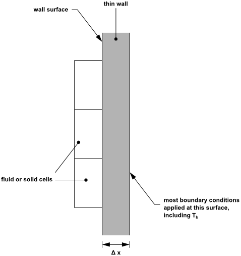
When postprocessing a wall that has a thickness but does not have shell conduction enabled, the Temperature... category provides three options: the temperature of the adjacent fluid / solid cells are stored as Static Temperature; the temperature of the wall surface itself is stored as Wall Temperature; and the temperature of the surface that is separated from the fluid / solid cells by the wall thickness is stored as Wall Temperature (Thin). If a more detailed analysis of the solid zone and surfaces is required, then you should consider creating layers of solid cells in your meshing application.
If the wall zone has a fluid or solid region on each side, it is called a “two-sided wall”. When you read a mesh with this type of wall zone into Ansys Fluent, a “shadow” zone will automatically be created so that each side of the wall is a distinct wall zone. In the Wall dialog box, the shadow zone’s name will be shown in the Shadow Face Zone field. You can choose to specify different thermal conditions on each zone, or to couple the two zones:
To couple the two sides of the wall (creating a "coupled wall"), select the Coupled option under Thermal Conditions. (This option will appear in the Wall dialog box only when the wall is a two-sided wall.) No additional thermal boundary conditions are required, because the solver will calculate heat transfer directly from the solution in the adjacent cells. You can, however, specify the material type, wall thickness, and heat generation rate for thin-wall thermal resistance calculations, as described in Thin-Wall Thermal Resistance Parameters. Note that the resistance parameters you set for one side of the wall will automatically be assigned to its shadow wall zone. Specifying the heat generation rate inside the wall is useful if, for example, you are modeling printed circuit boards where you know the electrical power dissipated in the circuits but not the heat flux or wall temperature.
Note:For inviscid flows with two-sided walls, the Thermal tab is greyed out and the reported heat flux on the CHT surface will be 0.
Results may differ for coupled walls that are intersecting boundaries. That is, you may see different results on a wall as compared to its wall-shadow depending on whether Node Values are enabled/disabled in this scenario.
To uncouple the two sides of the wall and specify different thermal conditions on each one, choose Temperature or Heat Flux as the thermal condition type (Convection and Radiation are not applicable for two-sided walls); note that this uncoupling will not be effective if you have enabled shell conduction for the wall. The relationship between the wall and its shadow will be retained, so that you can couple them again at a later time, if desired. You will need to set the relevant parameters for the selected thermal condition, as described above. The two uncoupled walls can have different thicknesses, and are effectively insulated from one another. If you specify a nonzero wall thickness for the uncoupled walls, the thermal boundary conditions you set will be specified for each thin wall on the surface that is separated from the fluid / solid cells by the wall thickness, as shown in Figure 7.57: Uncoupled Thin Walls, where
 is the Temperature (or
 is the Heat Flux) specified on
one wall and
is the Heat Flux) specified on
one wall and  is the Temperature (or
 is the Heat Flux) specified on
the other wall.
is the Heat Flux) specified on
the other wall.  and
and  are the thermal conductivities of the uncoupled thin
walls. Note that the gap between the walls in Figure 7.57: Uncoupled Thin Walls is not part of the model; it
is included in the figure only to show where the thermal boundary
condition for each uncoupled wall is applied.
are the thermal conductivities of the uncoupled thin
walls. Note that the gap between the walls in Figure 7.57: Uncoupled Thin Walls is not part of the model; it
is included in the figure only to show where the thermal boundary
condition for each uncoupled wall is applied.
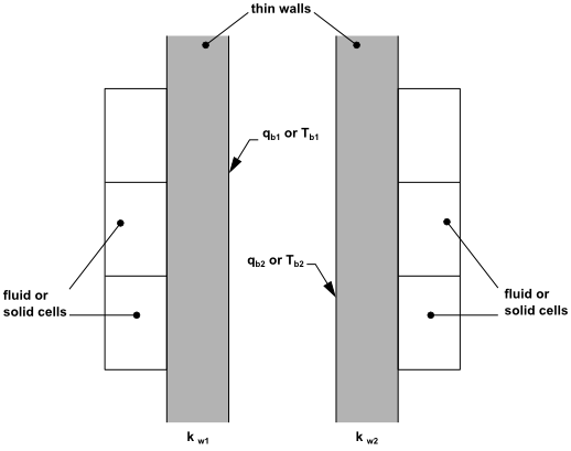
When cells near coupled two-sided walls have poor face orthogonality with respect to the wall, the tangential component (also known as the secondary gradient) of the discretized diffusive flux for the energy and user-defined scalar equations can become unbounded. This generates instabilities that can lead to solution divergence. When using the pressure-based solver, you have the option of limiting the secondary gradients in order to control the cross-diffusion source term. This control mechanism can improve the robustness of the discretization method while maintaining solution accuracy.
When this secondary gradient limiting is enabled, the diffusive flux
approximation (described in Connectivity Macros in the Fluent Customization Manual) at the wall is modified so that a coefficient
( ) controls the diffusion term:
 | (7–121) |
where the diffusion coefficient  is a function of face orthogonality—that is, the
dot product between
is a function of face orthogonality—that is, the
dot product between  (the area vector for the face, normal to the wall) and
 (the unit vector along the line connecting the cell
centroid (0) and face centroid (1)). Note that
(the unit vector along the line connecting the cell
centroid (0) and face centroid (1)). Note that  .
.
Note the following limitations:
It is only available with the pressure-based solver.
It can only be applied to the energy calculation and/or user-defined scalars (UDS) on coupled two-sided walls (that is, wall / wall-shadow pairs with Coupled selected from the Thermal Conditions list in the Thermal tab).
To enable orthogonality-based secondary gradient limiting, use the following text commands:
For the energy equation:
solve→set→advanced→secondary-gradient-limiting→energy?For user-defined scalars:
solve→set→advanced→secondary-gradient-limiting→uds?
When you enable secondary gradient limiting, by default it is applied to faces on the coupled two-sided walls using mesh quality limits from 0.7–0.9. You can shift the range if necessary by using the following text command; note that shifting this range closer to 1 will decrease the risk of divergence, but at the cost of accuracy.
solve → set
→ advanced →
secondary-gradient-limiting →
mesh-quality-limits
If the wall is not between two cell zones but is adjacent only to a single solid cell zone that involves solid motion with a nonzero translational or rotational velocity, then the Boundary Advection option is available. If the velocity for the solid motion (specified in the Solid Motion tab in the Solid dialog box) is directed into or out of the domain to a significant degree on that wall, then you should consider enabling the Boundary Advection option. This option allows you to account for the advection of thermal energy into or out of the solid domain at a rate that is consistent with the velocity normal to the boundary, the temperature of the material, and the material properties.
As an alternative to setting this option for each individual wall, you can use the following text command to review all the walls and automatically enable the Boundary Advection option where needed. The option is enabled on every appropriate wall for which the average angle of the velocity of the solid is greater than 2 degrees.
define →
boundary-conditions →
detect-boundary-advection
For details on setting up the solid motion model for a domain, see Defining Zone Motion.
To enable shell conduction for a wall, enable the Shell Conduction option in the Wall boundary condition dialog box. You can then click the button to open the Shell Conduction Layers dialog box, where you can define the properties of the single or multiple layers of the shell. Note that you must specify a nonzero wall thickness for every layer of the shell. When shell conduction is enabled, Ansys Fluent will compute heat conduction for the wall not only in the normal direction (which is always computed when the energy equation is solved), but also in the planar directions. The Shell Conduction option will appear in the Wall dialog box for all walls when solution of the energy equation is active (except for mapped interfaces). For information about how the thermal conditions are applied on a wall with shell conduction enabled, managing multiple shells, and postprocessing shell conduction walls, see Shell Conduction.
Ansys Fluent cases with shell conduction can be read in serial or parallel. Either a partitioned or an unpartitioned case file can be read in parallel (see Mesh Partitioning and Load Balancing for more information on partitioning). After reading a case file in parallel, shell zones can be created on any wall.
To convert every wall with a finite thickness into a shell with a single
action, the TUI command
define/boundary-conditions/modify-zones/create-all-shell-threads
can be used; each converted shell will have a single layer with the same
thickness as the original thin wall (any pre-existing shells will not be
modified). To disable shell conduction in every wall with a single action, the
TUI command
define/boundary-conditions/modify-zones/delete-all-shells
can be used. These capabilities are available in both serial and parallel
mode.
For more information on shell conduction, see Shell Conduction.
System Coupling allows the input and output of thermal data from Ansys Fluent. When Fluent is coupled with another system in Workbench using System Coupling, you can select the via System Coupling option on the desired wall boundaries to receive thermal data through System Coupling service. Note that this option does not need to be selected to provide thermal data from Fluent.
For more details about setting up a simulation with System Coupling, see the Performing System Coupling Simulations Using Fluent and the System Coupling User's Guide.
When thermal data is transferred into Fluent via System Coupling, the following variables are available:
temperature
heat flow (heat rate)
heat transfer coefficient (also known as "convection coefficient")
When thermal data is transferred out of Fluent via System Coupling, the following variables are available:
temperature
heat flow (heat rate)
heat transfer coefficient (also known as "convection coefficient")
near wall temperature (also known as "bulk temperature" or "ambient temperature")
For each data transfer, you specify the type of data transfer (the variables transferred) during the System Coupling setup.
As part of standard heat transfer boundary condition settings in Ansys Fluent, you can also specify the type of material, the thickness of the wall, and the heat generation rate in the wall. Select the material type in the Material Name drop-down list; if you want to check or modify the properties of the selected material, you can click to open the Edit Material dialog box (this dialog box contains just the properties of the selected material, and not the full contents of the standard Create/Edit Materials dialog box). You can specify the thickness in the Wall Thickness number-entry box and the heat generation rate in the Heat Generation Rate number-entry box.
Note: A boundary will behave in the same way as an adiabatic boundary if the via System Coupling option is enabled on this boundary, and Ansys Fluent is not receiving data from the coupling data transfer. Fluent is not receiving coupling data if it is either not involved with a System Coupling simulation, or if the coupling is a one-way transfer with the Fluent analysis only providing data to the second solver.
Mapped interfaces provide a robust approach for modeling coupled walls between zones when the interface zones penetrate each other or have gaps between them (see Figure 7.58: 2D Interface with Penetration and Gaps). For the interface wall boundary zones created as part of such interfaces, via Mapped Interface is automatically selected from the Thermal Conditions list in the Thermal tab of the Wall dialog box, in order to interpolate the thermal data.
Important: Note that thermal coupling calculations will not be performed at mapped interfaces for the Eulerian multiphase model.
For more details about mapped interfaces, see The Mapped Option and Using a Non-Conformal Mesh in Ansys Fluent.
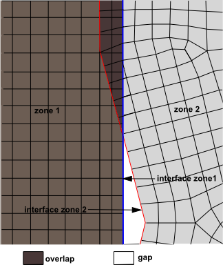
Such boundaries also allow you to specify the standard heat transfer boundary condition settings, such as the type of material, the thickness of the wall, and the heat generation rate in the wall. Select the material type in the Material Name drop-down list; if you want to check or modify the properties of the selected material, you can click to open the Edit Material dialog box (this dialog box contains just the properties of the selected material, and not the full contents of the standard Create/Edit Materials dialog box). You can specify the thickness in the Wall Thickness number-entry box and the heat generation rate in the Heat Generation Rate number-entry box. Note that the Shell Conduction option is not available with the via Mapped Interface thermal condition.
In the rarefied regime, the parietal gas temperature may differ from the imposed wall temperature. For details, see Temperature Jump for Rarefied Gases.
By default, a zero mass flux condition for all species is assumed at walls (except for species that participate in surface reactions). You can change the default settings and specify species mass fractions or non-zero mass fluxes at walls in your simulation. That is, both Dirichlet and Neumann boundary conditions such as those that are specified at inlets can be used at walls as well.
To change the default zero mass flux boundary condition for a species at the wall:
In the Wall Dialog Box, go to the Species tab to view the species boundary conditions for the wall (see Figure 7.59: The Wall Dialog Box for Species Boundary Condition Input).
In the Species Boundary Condition group box, you can define one of the following boundary conditions for the species at the wall:
If you want to specify a non-zero species mass flux, select Specified Mass Flux (default) in the drop-down list to the right of the species name. Then in the Species Mass Fraction / Mass Flux group box, enter its value for the species of interest.
Similarly, if you want to specify a species mass fraction, select Specified Mass Fraction in the drop-down list to the right of the species name. Then in the Species Mass Fraction / Mass Flux group box, enter its value for the species of interest.
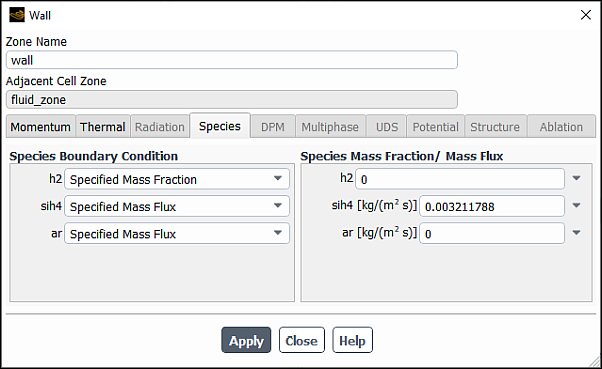
The boundary condition type for each species is specified separately, so you can choose to use different methods for different species.
If you are modeling species transport with Wall Surface reactions enabled in the Species Model dialog box, you can alternatively enable a reaction mechanism at a wall by selecting the Reaction option and then selecting an available mechanism from the Reaction Mechanisms drop-down list. See Defining Zone-Based Reaction Mechanisms for more information about defining reaction mechanisms.
You can also model unresolved surface washcoats, which greatly increase the catalytic surface area, by specifying the Surface Area Washcoat Factor. The surface washcoat increases the area available for surface reaction.
In transient simulations, if you want to postprocess the deposition of the solid species on the wall over time, you need to specify the following parameters:
Initial Deposition Thickness: is the thickness of the solid species deposition on the wall at the start of the simulation.
Solid Species Density: is the density of the solid species deposited on the wall. If more than one solid species exist in your simulation, then you need to specify the average solid species density.
Note that these two parameters are used for postprocessing purposes only and will not affect simulation results.
In hypersonic flows, the recombination of atoms is usually dominant at the wall. The atoms that diffuse to the wall can either reflect from the wall or recombine into molecules, see Partial Catalytic Boundary Condition for Walls.
If you are using the gray P-1, DTRM, DO, surface-to-surface, or MC models, you will need to set the emissivity of the wall (Internal Emissivity) in the Thermal tab of the Wall dialog box. If you are using the Rosseland model you do not need to set the emissivity, because Ansys Fluent assumes the emissivity is 1.
For the non-gray P-1, DO, or MC models, specify a constant Internal Emissivity for each wavelength band in the Radiation tab of the Wall dialog box (the default value in each band is 1). Alternatively, you can specify the internal emissivity using a boundary condition parameter (see Creating a New Parameter). If you are using the non-gray DO or MC models, you will also need to define the wall as opaque or semi-transparent in the Radiation tab. See Defining Boundary Conditions for Radiation for details. If you are using the DO or MC models, you can enable a Boundary Source.
If you are modeling a discrete phase of particles, you can set the fate of particle trajectories at the wall in the DPM section of the Wall dialog box. See Setting Boundary Conditions for the Discrete Phase for details.
If you are using the VOF model and you are modeling wall adhesion, you can specify the contact angle for each pair of phases at the wall in the Momentum tab of the Wall dialog box. See Steps for Setting Boundary Conditions for details.
If you have defined UDS transport equations in your model, you can specify boundary conditions for each equation in the UDS section of the Wall dialog box. See Setting Up UDS Equations in Ansys Fluent for details.
If you are using the Eulerian Wall Film model (see Modeling Eulerian Wall Films for details), you can set liquid film conditions at the wall in the Wall Film tab of the Wall dialog box. This tab is available only if you have enabled the Eulerian Wall Film model in the Models Task Page.
For details, see Setting Eulerian Wall Film Solution Controls.
For an intrinsic fluid-structure interaction (FSI) simulation, you can set the displacement boundary condition settings for walls that are adjacent to solid cell zones in the Structure tab of the Wall dialog box. This tab is only available when a model is selected in the Structural Model Dialog Box. For details, see Setting Up an Intrinsic Fluid-Structure Interaction (FSI) Simulation.
The default thermal boundary condition is a fixed heat flux of zero. Walls are, by default, not moving.
For no-slip wall conditions, Ansys Fluent uses the properties of the flow adjacent to the wall/fluid boundary to predict the shear stress on the fluid at the wall. In laminar flows this calculation simply depends on the velocity gradient at the wall, while in turbulent flows one of the approaches described in Near-Wall Treatments for Wall-Bounded Turbulent Flows in the Theory Guide is used.
For specified-shear walls, Ansys Fluent will compute the tangential velocity at the boundary.
If you are modeling inviscid flow with Ansys Fluent, all walls use a slip condition, so they are frictionless and exert no shear stress on the adjacent fluid.
In a laminar flow, the wall shear stress is defined by the normal gradient of the tangential velocity at the wall:
 | (7–122) |
When there is a steep velocity gradient at the wall, you must be sure that the mesh is sufficiently fine to accurately resolve the boundary layer. Guidelines for the appropriate placement of the near-wall node in laminar flows are provided in Mesh Element Distribution.
Wall treatments for turbulent flows are described in Near-Wall Treatments for Wall-Bounded Turbulent Flows in the Theory Guide.
When a fixed temperature condition is applied at the wall, the heat flux to the wall from a fluid cell is computed as
 | (7–123) |
| where | |
 = fluid-side local heat transfer coefficient = fluid-side local heat transfer coefficient | |
 = wall surface temperature = wall surface temperature | |
 = local fluid temperature = local fluid temperature | |
 = radiative heat flux = radiative heat flux |
Note that the fluid-side heat transfer coefficient is computed based on the local flow-field conditions (for example, turbulence level, temperature, and velocity profiles), as described by Equation 7–130.
Heat transfer to the wall boundary from a solid cell is computed as
 | (7–124) |
| where | |
 = thermal conductivity of the solid = thermal conductivity of the solid | |
 = local solid temperature = local solid temperature | |
 = distance between wall surface and the solid cell center = distance between wall surface and the solid cell center |
When you define a heat flux boundary condition at a wall, you specify the heat flux at the wall surface. Ansys Fluent uses Equation 7–123 and your input of heat flux to determine the wall surface temperature adjacent to a fluid cell as
 | (7–125) |
where, as noted above, the fluid-side heat transfer coefficient is computed based on the local flow-field conditions. When the wall borders a solid region, the wall surface temperature is computed as
 | (7–126) |
When you specify a convective heat transfer coefficient boundary condition at a wall, Ansys Fluent uses your inputs of the external heat transfer coefficient and external heat sink temperature to compute the heat flux to the wall as
 | (7–127) |
| where | |
 = external heat transfer coefficient defined by you = external heat transfer coefficient defined by you | |
 = external heat-sink temperature defined by you = external heat-sink temperature defined by you | |
 = radiative heat flux = radiative heat flux |
Equation 7–127 assumes a wall of zero-thickness.
When the external radiation boundary condition is used in Ansys Fluent, the heat flux to the wall is computed as
 | (7–128) |
| where | |
 = emissivity of the external wall surface defined by you = emissivity of the external wall surface defined by you | |
 = Stefan-Boltzmann constant = Stefan-Boltzmann constant | |
 = surface temperature of the wall = surface temperature of the wall | |
 = temperature of the radiation source or sink on the exterior of the domain, defined by
you = temperature of the radiation source or sink on the exterior of the domain, defined by
you | |
 = radiative heat flux to the wall from within the domain = radiative heat flux to the wall from within the domain |
Equation 7–128 assumes a wall of zero-thickness.
When you choose the combined external heat transfer condition, the heat flux to the wall is computed as
 | (7–129) |
where the variables are as defined above. Equation 7–129 assumes a wall of zero-thickness.
In laminar flows, the fluid side heat transfer at walls is computed using Fourier’s law applied at the walls. Ansys Fluent uses its discrete form:
 | (7–130) |
where  is the local coordinate normal to the wall.
For turbulent flows, Ansys Fluent uses the law-of-the-wall for temperature derived using the analogy between heat and momentum transfer [84]. See Standard Wall Functions in the separate Theory Guide for details.
Perforated walls can be used to introduce low-temperature air into a region operating under very high temperatures to provide efficient cooling of the walls. This is one of the most common techniques used in many industrial applications, such as combustor chambers.
Because perforated walls often have thousands of small holes, resolving every single hole is not practical due to the high computational cost. Ansys Fluent offers a model to account for the effects of air streams injected through the perforated holes.
Note the following limitations of the perforated wall model:
The perforated wall model considers the effects of perforated holes only on:
velocity fields
temperature fields (if the energy equation is enabled)
species distribution (if the species transport model is enabled)
mixture fraction and progress variable distribution (if the PDF model is enabled)
The perforated wall model is not supported with the density-based solver.
When the Euler-Euler multiphase flow model is used, the perforated wall model is applied only to the primary phase.
The effects of the perforated wall model on turbulence are not considered.
When modeling the effects of perforated holes in Ansys Fluent, solid walls are not meshed (except for cases that involve conjugate heat transfer as further described). Instead, a flow injection is imposed on the side where the flow is coming out through the perforated hole (hereinafter referred to as the injection side). In order to ensure the mass conservation, the same amount of mass flow is extracted at the side where the flow is coming into the perforated hole (hereinafter referred to as the extraction side).
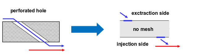
From the perspective of how the perforated walls are treated, there are two approaches to modeling the effects of perforated holes in the flow fields:
Uniform approach
Discrete approach
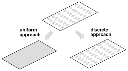
The uniform approach models the average effect of perforated walls on the flow field. Solid walls with the large number of the perforated holes are treated as having uniform injection conditions. The individual perforated hole is not resolved. Instead, the entire surface of the injection side wall has the same boundary condition of a prescribed mass flux. This approach is based on the rationale that in the preliminary design process, only the first-order effects of perforated walls on the flow field are of interest. This means that only the inviscid streamwise momentum flux and inviscid normal momentum flux due to injection are to be considered.
The discrete approach has more fidelity in modeling perforation holes effects. The individual perforated hole is resolved. In other words, the injections conditions are only imposed at the location of the perforated holes. Although this approach is able to resolve the flow fields at the individual perforated hole level, it does not imply that you need to actually mesh the holes during the meshing process. Instead, all the perforated holes can be marked via the perforated wall model capability in Ansys Fluent as described in Setting Perforated Walls.
Physically, if the perforated holes are fully resolved, the injection conditions at the exit of the holes are determined
internally by the flow inside the perforated channel. More specifically, they are determined by the pressure difference between
the extraction and injection sides. Therefore, the injection mass flow rate at the hole exit  (in kg/s) can be calculated by [14]:
 | (7–131) |
where
 = effective area of the hole channel = effective area of the hole channel |
 = discharging coefficient = discharging coefficient |
 = density on the extraction side = density on the extraction side |
 and and  = pressures on the extraction side and injection side, respectively = pressures on the extraction side and injection side, respectively |
In order to determine the injection mass flow rate, the value of the discharging coefficient  must be specified. In some practical scenarios, the product value of
  may be known instead of individual values of
  and
and  . In Ansys Fluent, you can specify either
  or
or  as described in Setting Perforated Walls.
Equation 7–131 assumes that the flow inside the perforated channel is incompressible. If the speed inside the perforated channel is very high, the compressible flow is more adequate to describe the flow behaviors under this circumstance. A compressible formulation for the injection condition is suggested as [11]:
 | (7–132) |

where
 = gas constant = gas constant |
 = temperature of the extraction side = temperature of the extraction side |
 = heat capacity ratio = heat capacity ratio |
Estimating injection condition based on Equation 7–131 or Equation 7–132 is referred to
as the dynamic method in Ansys Fluent since the injection mass flow rate is estimated based on the local pressure field. Besides the
dynamic injection method specification, you can directly specify the injection mass flow rate at the hole exit (in kg/s). This is referred to as the static injection method in Ansys Fluent.
Once the injection mass flow rate is determined via either the dynamic or static injection method, a proper mass flux condition is imposed on the extraction side to ensure mass conservation. After the mass flux condition is determined on the extraction side, the amount of energy and species (or mixture fraction/progress variable) removed on the extraction side can be calculated. As a result, the same amount of energy and species is added on the injection side to ensure energy conservation and species mass conservation. For the momentum flux on the injection side, different options can be selected based on the application need.
Note that although the perforated wall model originally comes from the gas turbine combustor applications, it is also applicable to general problems if similar effects on the flow fields need to be accounted for.
For conjugate heat transfer cases, solid walls are meshed, while perforated holes are not meshed. The effects of perforated holes in the flow fields is modeled using the discrete approach. The injection mass flow rate at the hole exit is still calculated by Equation 7–131. The heat transfer effects between the solid walls and the flow when the injection flow passes through the perforated holes can be accounted for as described below. An example of such a problem is conjugate heat transfer in a gas turbine combustor where low-temperature air passing through perforated holes is heated due to the higher-temperature solid walls.
The heat transfer between the solid walls and the injection flow  is calculated by:
 | (7–133) |
where
 and and  = diameter and length of the perforated hole,
respectively = diameter and length of the perforated hole,
respectively |
 = flow temperature at the entrance of the perforated
hole = flow temperature at the entrance of the perforated
hole |
 = solid wall temperature = solid wall temperature |
 = convection heat transfer coefficient = convection heat transfer coefficient |
 is calculated by Cho and Goldstein’s correlation for
short-length holes [11]:
is calculated by Cho and Goldstein’s correlation for
short-length holes [11]:
 | (7–134) |
where
 = Nusselt number = Nusselt number |
 = thermal conductivity of the fluid = thermal conductivity of the fluid |
 and and  = Reynolds number and Prandtl number, respectively = Reynolds number and Prandtl number, respectively |
With Equation 7–133, the injection flow temperature at the
hole exit  is calculated by:
 | (7–135) |
where  is the injection mass flow rate given by Equation 7–131, and
  is the heat capacity of the fluid.
As the perforated holes are not meshed, the solid wall temperature  in Equation 7–133 is estimated as follows.
Given that the solid walls are relatively thin and have large thermal conductivity,
the solid wall temperature is assumed to be linearly distributed in the direction of
the orientation of the perforated holes. Then the analytical solution for the total
heat transfer can be expressed as:
in Equation 7–133 is estimated as follows.
Given that the solid walls are relatively thin and have large thermal conductivity,
the solid wall temperature is assumed to be linearly distributed in the direction of
the orientation of the perforated holes. Then the analytical solution for the total
heat transfer can be expressed as:
 | (7–136) |
with
 | (7–137) |
In Equation 7–136,  and
and  are the wall temperature at the entrance and exit of perforated
holes, respectively.
are the wall temperature at the entrance and exit of perforated
holes, respectively.
If you want to consider the effects of air streams injected through the perforated holes in your simulation, follow the below steps. Note that the perforated walls model setup is based on the injection side; the extraction side will be handled automatically by Ansys Fluent based on the selected model options.
In the Boundary Conditions task page, click the Perforated Wallis... button.
In the Perforated Walls dialog box that opens, enable the Perforated Wall Model option.
Select an appropriate Model Setup Method from the following options:
- Import Input Files
allows you to read an input file that contains the selections of model options and values of the model parameters. This option is useful for cases where hundreds or even thousands of perforated holes need to be defined.
- Manual Inputs
allows you to manually specify perforated wall options and parameters. When this option is selected, the Perforated Walls dialog box expands to reveal relevant model inputs.
If you have chosen Import Input File, use the Select File dialog box to read an input file for the perforated wall definition. See Perforated Wall File Format for the details about input file format and an example of the perforated wall file.
Once Ansys Fluent reads the file, the data entry fields in the Injection Holes and Dynamic Setup dialog boxes will be automatically populated with the appropriate information. You can review and edit these settings in each dialog box.
If you have chosen Manual Inputs, follow the steps outlined in Procedure for Manual Setup of Perforated Walls:
Click to close the Perforated Walls dialog box.
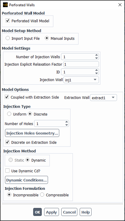
If you have chosen the Manual Inputs option in the Perforated Walls dialog box (Model Setup Method group box), you need to specify the following settings and options:
In the Model Settings group box (see Figure 7.62: The Perforated Walls Dialog Box), specify the total number of walls where you want to define the perforated wall boundary condition in the Number of Injection Walls field. You will need to define boundary conditions for each wall separately.
In the Injection Explicit Relaxation Factor field, enter a value between 0 and 1 (default = 1).
This parameter controls the update of the injection mass flow rate at each iteration. It is used to blend the injection mass flow rates calculated by Equation 7–131 (for an incompressible flow) or Equation 7–132 (for a compressible flow) at the current and previous iterations. If any convergence issues arise, you can try to lower this factor at the beginning of your run.
Set the ID of the injection wall. This number must be between 1 and the value specified in Number of Injection Walls.
From the Injection Wall drop-down list, select the name of the injection wall you are defining.
If you want to couple the injection and extraction walls, enable Coupled with Extraction Side.
With Coupled with Extraction Side enabled, Ansys Fluent automatically selects Dynamic in the Injection Method group box. Otherwise, Ansys Fluent uses the Static injection method.
Note: In the current implementation, you cannot change the injection method (Static or Dynamic).
Select the name of the extraction wall that you want to couple with the injection wall from the Extraction Wall drop-down list (Modeling Options group box). When the flow is introduced on the injection wall, the same amount of mass is removed from the extraction wall.
In the Injection Type group box select either Uniform or Discrete modeling approach. See Modeling Concept for more information about these two approaches.
For the Discrete injection type, define the geometry of the injection holes.
In the Number of Holes field, set the total number of perforated holes in the injection wall.
Click the Injection Holes Geometry... button to specify the injection holes parameters in the Injection Holes dialog box that opens.
Select the Axes Specification Method for defining perforated holes:
- Point-Point
allows you to specify two arbitrary points on the cylinder axis.
- Point-Direction
allows you to specify a point and a direction vector of the cylinder axis.
For each hole with the ID set in the Hole ID field, you need to specify the following parameters in the Hole Geometry group box (depending on your selection of the Axes Specification Method):
For the Point-Point axes specification method:
Coordinates of two points on the cylinder axis (( Point 1 X, Point 1 Y, Point 1 Z) and (Point 2 X, Point 2 Y, Point 2 Z))
Diameter
For the Point-Direction axes specification method:
Coordinates of a point on the cylinder axis (Point X, Point Y, Point Z) and a direction vector (Direction X, Direction Y, Direction Z)
Diameter
Note: Inputs for the Z coordinate will be displayed for 3D cases only.
Ansys Fluent will automatically find all intersections between the specified cylinders and the injection or extraction wall. Then each face involved in the intersections will be marked as either a hole exit or a hole inlet, respectively.
Click to close the Injection Holes dialog box.
If you want to model the uniform condition on the extraction side, disable the Discrete on Extraction Side option (default) (Injection Type group box).
For the Static injection method, specify the static method settings.
In the Injection Method group box, click the Static Conditions... button to specify injection settings in the Static Setup dialog box that opens.
Select the Specification Method from the following options:
- Normal to Boundary
defines the injection direction by the normal to the surface of the injection wall.
- Direction
defines the injection direction by the three components of the directional vector.
For each hole with the ID set in the Hole ID field, you need to specify the following parameters in the Static Method Parameters group box:
Mass Flow Rate: Injection mass flow rate (kg/s)
Temperature: Injection static temperature (K)
Mass fractions of species that constitute the mixture material in the injection flow
In the example shown in Figure 7.64: The Static Setup Dialog Box (Uniform Injection), the mixture material contains H 2 O, O 2, and N 2. In this case, the mixture fraction of h2o and o2 must be specified. The mass fraction of N 2 is computed by subtracting the sum of the remaining mass fractions from unity.
( Direction specification method only) X Direction, Y Direction, and Z Direction (3D only)
Click to close the Static Setup dialog box.
For the Dynamic injection method, specify the dynamic method settings.
In the Injection Method group box, click the Dynamic Conditions... button to specify injection settings in the Dynamic Setup dialog box that opens.
If you have selected the Uniform injection type, you need to specify the following:
Select the Dynamic Method Parameter from the following options:
- Normal to Boundary
defines the injection direction by the normal to the surface of the injection wall.
- Direction
defines the injection direction by the three components of the directional vector.
- Injection Angles
defines the injection direction by the surface and tangential angles. These are the angles of the cylinder axis
 and
and  in the local cylindrical coordinate system (
 ,
,  ,
,  ) as shown in Figure 7.66: Injection Surface and Tangential Angles.
The directions of the local cylindrical coordinate system are:
 is the outward normal to the perforated wall surface
 has the same direction as the circumferential direction
 of the global cylindrical coordinate system (
 ,
,  ,
,  ), where
  and
and  are the axial and radial directions, respectively.
 is the direction of the cross product
  .
.
For each hole with the ID set in the Hole ID field, you need to specify the following parameters in the Dynamic Method Parameters group box (depending on your selection of the injection direction method):
For all injection direction methods: ACd (the coefficient
in Equation 7–131 for an incompressible flow or Equation 7–132 for a compressible flow)For the Direction method: Injection direction vector (X Direction, Y Direction, and Z Direction)
For the Injection Angles method: Injection direction angles (Surface Angle and Tangential Angle)
Click to close the Dynamic Setup dialog box.
If you have selected the Discrete injection type, you need to specify the following:
Select the Dynamic Method Parameter from the following options:
- Cd
is
in Equation 7–131 for an incompressible flow or Equation 7–132 for a compressible flow- ACd
Is
in Equation 7–131 for an incompressible flow or Equation 7–132 for an compressible flow
For each hole with the ID set in the Hole ID field, you need to enter the value for Cd (if you selected Cd for the Dynamic Method Parameter) or ACd (if you selected ACd for the Dynamic Method Parameter) in the Dynamic Method Parameters group box.
Click to close the Dynamic Setup dialog box.
Select the Injection Formulation (Injection Method group box) from the following options:
Incompressible: Uses Equation 7–131 to calculate the injection mass flow rate at the hole exit
Compressible: Uses Equation 7–132 to calculate the injection mass flow rate at the hole exit
(optional) By default, Ansys Fluent uses a constant value for
in Equation 7–131. For the Discrete injection type with
the Discrete on Extraction Side option, you can use a custom formulation for by selecting the Use Dynamic Cd? option and hooking your
DEFINE_PERFORATED_CDUDF to the code. SeeDEFINE_PERFORATED_CDin the Fluent Customization Manual for more information.
(cases with solid zone(s) only) If you want to simulate the effects of conjugate heat transfer between the solid walls and the injection flow, enable the CHT Coupling option. This option is available when the following options are enabled:
Coupled with Extraction Side (Model Options group box)
Discrete (Injection Type group box)
Discrete on Extraction Side (Injection Type group box)
Note that the Injection Wall and Extraction Wall must be coupled, that is, they should be a wall/wall-shadow-pair.
See Modeling Concept for more information about conjugate heat transfer coupling.
Repeat steps 3-11 for each wall ID where you want to define the perforated wall boundary condition.
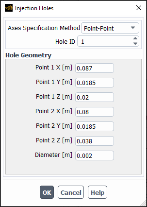
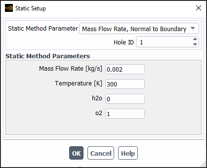
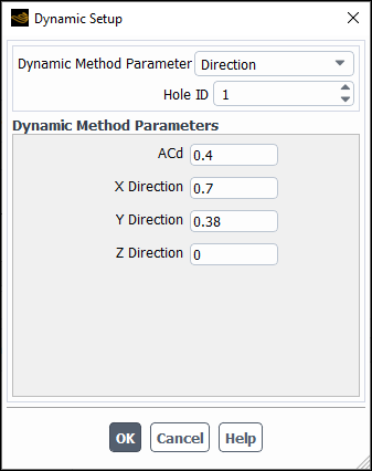
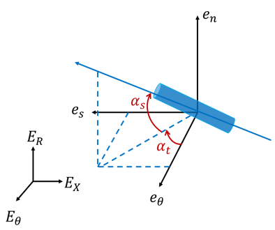
A perforated wall file is an ASCII file containing information for setting a perforated wall boundary condition on selected
walls. The file can contain comment lines, which are lines that begin with either a forward slash (/), a
semicolon (;), or an exclamation mark (!).
The following is an example of an input file that sets perforated wall boundary conditions on two walls for a 3D case:
// Sample Input File for Effusion Cooling Model
// total number of effusion walls (pairs)
2
// URF for mass flow calculations
0.6
//++++++++++++++++++++ First Pair ++++++++++++++++++++++++++++
// Injection Wall Name
effusion-down:002
// Coupling Method
// Format: coupled [extraction wall name]
coupled effusion-up
// Injection Type
// "uniform" or "discrete" [cylinder method] [discrete on extraction side?]
discrete point-point ext-discrete
// Injection Method
// "dynamic" [mass flow rate formulation] ("incompressible" or "compressible")
dynamic compressible
// Model Inputs
// The header line starts with a '%', the subsequent lines define injection parameters
%   x1       y1       z1       x2       y2       z2   diameter    cd
0.010000 0.001000 0.010000 0.005000 0.001000 0.011000 0.000500 0.500000
0.010000 0.002000 0.010000 0.005000 0.002000 0.011000 0.000500 0.500000
...
0.025000 0.010000 0.010000 0.020000 0.010000 0.011000 0.000500 0.500000
//+++++++++++++++++++++ Second Pair +++++++++++++++++++++++++++
// Injection Wall Name
effusion-down
// Coupling Method
// "coupled" [extraction wall name]
coupled effusion-up
// Injection Type
// "uniform" or "discrete" [cylinder method] [discrete on extraction side?]
discrete point-point ext-discrete
// Injection Method
// "dynamic" [mass flow rate formulation] ("incompressible" or "compressible")
dynamic compressible
// Model Inputs
// The header line starts with a '%', the subsequent lines define injection parameters
%   x1       y1       z1       x2       y2       z2   diameter    cd
0.032000 0.001000 0.010000 0.027000 0.001000 0.011000 0.000500 0.500000
0.032000 0.002000 0.010000 0.027000 0.002000 0.011000 0.000500 0.500000
...
0.042000 0.010000 0.010000 0.037000 0.010000 0.011000 0.000500 0.500000
The format of the perforated wall input file (excluding comment and blank lines) is as follows:
The first line contains the number of the walls to which you want to assign the perforated wall boundary condition (a single integer number). You will need to define each perforated wall separately.
Line 2 provides the injection explicit relaxation factor (a single float number between 0 and 1).
Line 3 is the name of the injection wall. Lines that follow Line 3 contain parameters that define the perforated wall boundary condition for this wall.
Line 4 contains the following keyword:
Model options:
coupledoruncoupled.(
coupledinjections only) The name of the coupled extraction wall.
Line 5 contains the following keywords:
Injection type:
uniformordiscrete(
discreteinjection type only) Perforated hole definition method:point-pointorpoint-direction(
uniforminjection type only) Injection direction definition method:normal(normal to boundary),direction(direction vector), orangle(injection angles)Optional keyword
ext-discretefor using the discrete condition on the extraction wall
In the above example, Line 5 specifies the
discreteinjection type, thepoint-pointhole definition method, and theext-discretecondition on the extraction wall.Line 6 contains the following keywords:
Injection method (
staticordynamic)(optional,
dynamicinjection method only)cd-profileto use a UDF to calculate in Equation 7–131. If this keyword is not present, Ansys Fluent uses a constant
value of .(
dynamicinjection method only) Mass flow rate formulation (incompressibleorcompressible) described in Equation 7–131 and Equation 7–132, respectively.(optional, cases with solid zone(s) only)
cht-couplingto consider the effects of heat transfer between the solid walls and the injection flow. This item is only valid forcoupleddiscreteinjections with thedynamicinjection method.
Line 7 begins with the percentage character (%) and contains the header information for the perforated wall inputs. The following keywords can be used in the header:
x, y, z, vx, vy, vz, x1, y1, z1, x2, y2, z2, diameter, nx, ny, nz, alpha-s, alpha-t, mf, tem, fmean, pv,species namesNote: The keyword and inputs for the Z coordinate are required for 3D cases only.
The keywords may be provided in any order. However, the hole and injection data in the subsequent lines must follow the order you have defined in the header line.
Depending on the selection of the injection type and dynamic conditions, different data must be provided as further described.
The subsequent lines describe perforated hole parameters. Each line contains input data for each individual hole. The input values and keywords in each line must follow the order you have specified in the header (Line 7). The inputs are described below along with the keywords that must appear in the header line:
(
discreteinjection type only) Hole geometry information:For the
point-pointhole definition method: the coordinates of two points on the hole axis and the diameter. The header keywords for these variables are:x1, y1, z1, x2, y2, z2, diameterFor the
point-directionhole definition method: the coordinates of the point on the hole axis, the direction vector, and the diameter. The header keywords are:x, y, z, vx, vy, vz, diameter
(both uniform and discrete injection types) Coefficient for the injection mass flow rate:
For the
uniforminjection type: (in Equation 7–131 or Equation 7–132). The
header keyword is acd.For the
discreteinjection type: either or (in Equation 7–131 or Equation 7–132). The
header keywords are respectively: cdoracd.
(
uniforminjection type only) Injection direction parameters:For the
directioninjection direction definition method: the coordinates of the direction vector. The header keywords are:nx,ny,nz.For the
angleinjection direction definition method: the surface angle and the tangential angle. The header keywords are:alpha-s,alpha-t.
(
staticinjection method only) Static injection parameters:Mass flow rate of injection wall. The header keyword is
mf.(if the energy equation is enabled) Temperature of the injection flow. The header keyword is
tem.(if the species transport model is enabled): Species mass fractions. The header keywords are the species names present in the mixture material. You only need to specify non-zero values of species mass fractions in the injection flow, and the rest of the species in the mixture are automatically assumed to have zero mass fractions.
(if the PDF turbulent combustion model is enabled): the mean mixture fraction and/or progress variable. The header keywords are
fmeanandpv, respectively.
For example, for the uniform injection with the
angledirection specification, each line must contain inputs for the following keywords:acd alpha-s alpha-tThe number of input lines determines the number of perforated holes in the wall.
If the perforated wall boundary condition is assigned to more than one wall in your case, provide information for each wall as described above.
When the perforated wall model is enabled, you can generate graphical plots or alphanumeric reports of the following field variables. These quantities are available in the Perforated Walls... category:
Tagged Face
Injection Hole Mass Flow Rate
Injection Pressure
Conjugate Heat Transfer
See Alphabetical Listing of Field Variables and Their Definitions for their definitions.
Symmetry boundary conditions are used when the physical geometry of interest, and the expected pattern of the flow/thermal solution, have mirror symmetry. They can also be used to model zero-shear slip walls in viscous flows. This section describes the treatment of the flow at symmetry planes and provides examples of the use of symmetry. You do not define any boundary conditions at symmetry boundaries, but you must take care to correctly define your symmetry boundary locations.
Important: At the centerline of an axisymmetric geometry, you should use the axis boundary type rather than the symmetry boundary type, as illustrated in Figure 7.74: Use of an Axis Boundary as the Centerline in an Axisymmetric Geometry. See Axis Boundary Conditions for details.
Symmetry boundaries are used to reduce the extent of your computational model to a symmetric subsection of the overall physical system. Figure 7.67: Use of Symmetry to Model One Quarter of a 3D Duct and Figure 7.68: Use of Symmetry to Model One Quarter of a Circular Cross-Section illustrate two examples of symmetry boundary conditions used in this way.
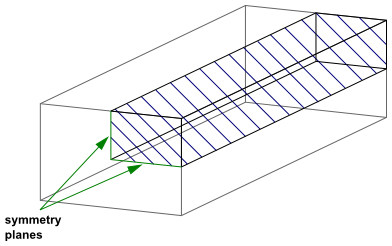
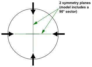
Figure 7.69: Inappropriate Use of Symmetry illustrates two problems in which a symmetry plane would be inappropriate. In both examples, the problem geometry is symmetric but the flow itself does not obey the symmetry boundary conditions. In the first example, buoyancy creates an asymmetric flow. In the second, swirl in the flow creates a flow normal to the would-be symmetry plane. Note that this second example should be handled using rotationally periodic boundaries (as illustrated in Figure 7.70: Use of Periodic Boundaries to Define Swirling Flow in a Cylindrical Vessel).
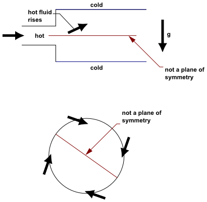
Ansys Fluent assumes a zero flux of all quantities across a symmetry boundary. There is no convective flux across a symmetry plane: the normal velocity component at the symmetry plane is therefore zero. There is no diffusion flux across a symmetry plane: the normal gradients of all flow variables are therefore zero at the symmetry plane. The symmetry boundary condition can therefore be summarized as follows:
zero normal velocity at a symmetry plane
zero normal gradients of all variables at a symmetry plane
As stated above, these conditions determine a zero flux across the symmetry plane, which is required by the definition of symmetry. Since the shear stress is zero at a symmetry boundary, it can also be interpreted as a “slip” wall when used in viscous flow calculations.
Periodic boundary conditions are used when the physical geometry of interest and the expected pattern of the flow/thermal solution have a periodically repeating nature. Two types of periodic conditions are available in Ansys Fluent. The first type does not allow a pressure drop across the periodic planes. (Note to FLUENT 4 users: This type of periodic boundary is referred to as a “cyclic” boundary in FLUENT 4.) The second type allows a pressure drop to occur across translationally periodic boundaries, enabling you to model “fully-developed” periodic flow. (In FLUENT 4 this is a “periodic” boundary.)
This section discusses the no-pressure-drop periodic boundary condition. A complete description of the fully-developed periodic flow modeling capability is provided in Periodic Flows.
Periodic boundary conditions are used when the flows across two opposite planes in your computational model are identical. Figure 7.70: Use of Periodic Boundaries to Define Swirling Flow in a Cylindrical Vessel illustrates a typical application of periodic boundary conditions. In this example the flow entering the computational model through one periodic plane is identical to the flow exiting the domain through the opposite periodic plane. Periodic planes are always used in pairs as illustrated in this example.
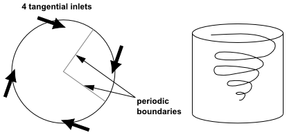
For a periodic boundary without any pressure drop, there is only one input you need to consider: whether the geometry is rotationally or translationally periodic. (Additional inputs are required for a periodic flow with a periodic pressure drop. See Periodic Flows.)
Rotationally periodic boundaries are boundaries that form an included angle about the centerline of a rotationally symmetric geometry. Figure 7.70: Use of Periodic Boundaries to Define Swirling Flow in a Cylindrical Vessel illustrates rotational periodicity. Translationally periodic boundaries are boundaries that form periodic planes in a rectilinear geometry. Figure 7.71: Example of Translational Periodicity - Physical Domain illustrates translationally periodic boundaries.
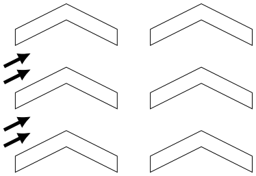
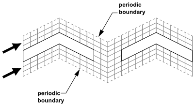
You will specify translational or rotational periodicity for a periodic boundary in the Periodic Dialog Box (Figure 7.73: The Periodic Dialog Box), which is opened from the Boundary Conditions task page (as described in Setting Cell Zone and Boundary Conditions).
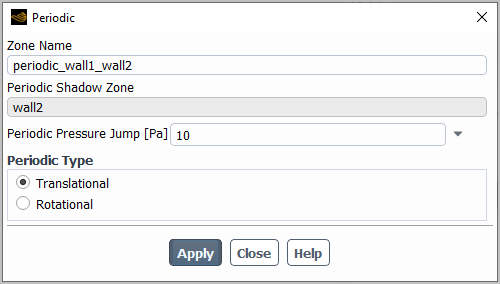
Note that there will be an additional item in the Periodic dialog box for the density-based solver, which allows you to specify the periodic pressure jump. See Periodic Flows for details.
If the domain is rotationally periodic, select Rotational as the Periodic Type; if it is translationally periodic, select Translational. For rotationally periodic domains, the solver will automatically compute the angle through which the periodic zone is rotated. The axis used for this rotation is the axis of rotation specified for the adjacent cell zone.
Note that there is no need for the adjacent cell zone to be moving for you to use a rotationally periodic boundary. You could, for example, model pipe flow in 3D using a stationary reference frame with a pie-slice of the pipe; the sides of the slice would require rotational periodicity.
Click the button in the Mesh group box of the Domain tab (see Checking the Mesh) to compute and display the minimum, maximum, and average rotational angles of all faces on periodic boundaries. If the difference between the minimum, maximum, and average values is not negligible, then there is a problem with the mesh: the mesh geometry is not periodic about the specified axis.
By default, all periodic boundaries are translational.
Ansys Fluent treats the flow at a periodic boundary as though the opposing periodic plane is a direct neighbor to the cells adjacent to the first periodic boundary. Therefore, when calculating the flow through the periodic boundary adjacent to a fluid cell, the flow conditions at the fluid cell adjacent to the opposite periodic plane are used.
The axis boundary type must be used as the centerline of an axisymmetric geometry (see Figure 7.74: Use of an Axis Boundary as the Centerline in an Axisymmetric Geometry ). It can also be used for the centerline of a cylindrical-polar quadrilateral or hexahedral mesh (for example, a mesh created for a structured-mesh code such as FLUENT 4). You do not need to define any boundary conditions at axis boundaries.
Important: When creating 2D axisymmetric geometry, the axis boundary must lie on the y=0 line.
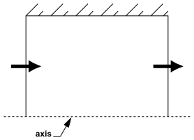
The fan model is a lumped parameter model that can be used to determine the impact of a fan with known characteristics upon some larger flow field. The fan boundary type allows you to input an empirical fan curve that governs the relationship between head (pressure rise) and flow rate (velocity) across a fan element. You can also specify radial and tangential components of the fan swirl velocity. The fan model does not provide an accurate description of the detailed flow through the fan blades. Instead, it predicts the amount of flow through the fan. Fans may be used in conjunction with other flow sources, or as the sole source of flow in a simulation. In the latter case, the system flow rate is determined by the balance between losses in the system and the fan curve.
Ansys Fluent also provides a connection for a special user-defined fan model that updates the pressure jump function during the calculation. This feature is described in User-Defined Fan Model.
The following are limitations when using fan boundary conditions:
By default, fan boundaries are included in the solar flux calculation when using the Solar Load model with no option to disable.
A fan is considered to be infinitely thin, and the discontinuous pressure rise across it is specified as a function of the velocity through the fan. The relationship may be a constant, a polynomial, piecewise-linear, or piecewise-polynomial function, or a user-defined function.
In the case of a polynomial, the relationship is of the form
 | (7–138) |
where  is the pressure jump,
  are the pressure-jump polynomial coefficients, and
  is the magnitude of the local fluid velocity normal to the fan.
Important: The velocity  can be either positive or negative. You must be careful to model the fan so that a pressure rise occurs
for forward flow through the fan.
can be either positive or negative. You must be careful to model the fan so that a pressure rise occurs
for forward flow through the fan.
You can, optionally, use the mass-averaged velocity normal to the fan to determine a single pressure-jump value for all faces in the fan zone.
For three-dimensional problems, the values of the convected tangential and radial velocity fields can be imposed on the fan surface to generate swirl. These velocities can be specified as functions of the radial distance from the fan center. The relationships may be constant or polynomial functions, or user-defined functions.
Important: You must use SI units for all fan swirl velocity inputs.
For the case of polynomial functions, the tangential and radial velocity components can be specified by the following equations:
 | (7–139) |
 | (7–140) |
where  and
and  are, respectively, the tangential and radial velocities on the fan surface in m/s,
  and
and  are the tangential and radial velocity polynomial coefficients, and
  is the distance to the fan center.
Once the fan zone has been identified (in the Boundary Conditions task page), you will set all modeling inputs for the fan in the Fan Dialog Box (Figure 7.75: The Fan Dialog Box), which is opened from the Boundary Conditions Task Page (as described in Setting Cell Zone and Boundary Conditions).
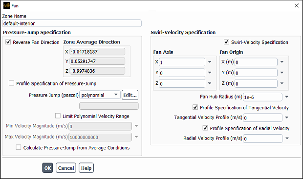
Inputs for a fan are as follows:
Identify the fan zone.
Define the pressure jump across the fan.
Define the discrete phase boundary condition for the fan (for discrete phase calculations).
Define the swirl velocity, if desired (3D only).
Since the fan is considered to be infinitely thin, it must be modeled as the interface between cells, rather than a cell zone. Therefore the fan zone is a type of internal face zone (where the faces are line segments in 2D or triangles/quadrilaterals in 3D). If, when you read your mesh into Ansys Fluent, the fan zone is identified as an interior zone, right-click the zone in the tree and use the Type sub-menu to change it to a fan zone (for more details, see Changing Cell and Boundary Zone Types).
Once the interior zone has been changed to a fan zone, you can open the Fan dialog box and specify the pressure jump and, optionally, the swirl velocity.
To define the pressure jump, you will specify a polynomial, piecewise-linear, or piecewise-polynomial function of velocity, a user-defined function, or a constant value. You should also check the Zone Average Direction vector to be sure that a pressure rise occurs for forward flow through the fan. The Zone Average Direction, calculated by the solver, is the face-averaged direction vector for the fan zone. If this vector is pointing in the direction you want the fan to blow, do not select Reverse Fan Direction; if it is pointing in the opposite direction, select Reverse Fan Direction.
Follow these steps to set a polynomial, piecewise-linear, or piecewise-polynomial function for the pressure jump:
Check that the Profile Specification of Pressure-Jump option is off in the Fan Dialog Box.
Choose polynomial, piecewise-linear, or piecewise-polynomial in the drop-down list to the right of Pressure-Jump. (If the function type you want is already selected, you can click the button to open the dialog box where you will define the function.)
In the dialog box that appears for the definition of the Pressure Jump function (for example, Figure 7.76: Polynomial Profile Dialog Box for Pressure Jump Definition), enter the appropriate values. These profile input dialog boxes are used the same way as the profile input dialog boxes for temperature-dependent properties. See Defining Properties Using Temperature-Dependent Functions to find out how to use them.
Set any of the optional parameters described below. (optional)
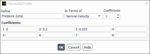
When you define the pressure jump using any of these types of functions, you can choose to limit the minimum and maximum velocity magnitudes used to calculate the pressure jump. Enabling the Limit Polynomial Velocity Range option limits the pressure jump when a Min Velocity Magnitude and a Max Velocity Magnitude are specified.
Important: The values corresponding to the Min Velocity Magnitude and the Max Velocity Magnitude do not limit the flow field velocity to this range. However, this range does limit the value of the pressure jump, which is a polynomial and a function of velocity, as seen in Equation 7–138. If the calculated normal velocity magnitude exceeds the Max Velocity Magnitude that has been specified, then the pressure jump at the Max Velocity Magnitude value will be used. Similarly, if the calculated velocity is less than the specified Min Velocity Magnitude, the pressure jump at the Min Velocity Magnitude will be substituted for the pressure jump corresponding to the calculated velocity.
You also have the option to use the mass-averaged velocity normal to the fan to determine a single pressure-jump value for all faces in the fan zone. Turning on Calculate Pressure-Jump from Average Conditions enables this option.
To define a constant pressure jump, follow these steps:
Turn off the Profile Specification of Pressure-Jump option in the Fan Dialog Box.
Choose constant in the drop-down list to the right of Pressure-Jump.
Enter the value for
 in the Pressure-Jump field.
You can follow the procedure below, if it is more convenient:
Turn on the Profile Specification of Pressure-Jump option.
Select constant in the drop-down list below Pressure Jump Profile, and enter the value for
 in the Pressure Jump Profile field.
For a user-defined pressure-jump function or a function defined in a boundary profile file, you will follow these steps:
Turn on the Profile Specification of Pressure-Jump option.
Choose the appropriate function in the drop-down list below Pressure Jump Profile.
Important: The profile must be written in ascending order with smallest pressure jump listed at the top. See Example: Determining the Pressure Jump Function.
See the Fluent Customization Manual for information about user-defined functions, and Profiles for details about profile files.
This example shows you how to determine the function for the pressure jump. Consider the simple two-dimensional duct
flow illustrated in Figure 7.77: A Fan Located In a 2D Duct. Air at constant density enters the 2.0 m  0.4 m duct with a velocity of 15 m/s. Centered in the duct is a fan.
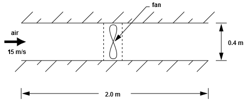
Assume that the fan characteristics are as follows when the fan is operating at 2000 rpm:
 ( ( /s) /s)
|  (Pa) (Pa)
|
| 25 | 0.0 |
| 20 | 175 |
| 15 | 350 |
| 10 | 525 |
| 5 | 700 |
| 0 | 875 |
where  is the flow through the fan and
  is the pressure rise across the fan. The fan characteristics in this example follow a simple linear
relationship between pressure rise and flow rate. To convert this into a relationship between pressure rise and velocity,
the cross-sectional area of the fan must be known. In this example, assuming that the duct is 1.0 m deep, this area is 0.4
m 2, so that the corresponding velocity values are as follows:
is the pressure rise across the fan. The fan characteristics in this example follow a simple linear
relationship between pressure rise and flow rate. To convert this into a relationship between pressure rise and velocity,
the cross-sectional area of the fan must be known. In this example, assuming that the duct is 1.0 m deep, this area is 0.4
m 2, so that the corresponding velocity values are as follows:
 (m/s) (m/s)
|  (Pa) (Pa)
|
|
62.5 |
0.0 |
| 50.0 | 175 |
| 37.5 | 350 |
| 25.0 | 525 |
| 12.5 | 700 |
| 0 | 875 |
The polynomial form of this relationship is the following equation for a line:
 | (7–141) |
If you are modeling a discrete phase of particles, you can set the fate of particle trajectories at the fan. See Setting Boundary Conditions for the Discrete Phase for details.
If you want to set tangential and radial velocity fields on the fan surface to generate swirl in a 3D problem, follow these steps:
Turn on the Swirl-Velocity Specification option in the Fan Dialog Box.
Specify the fan’s axis of rotation by defining the axis origin (Fan Origin) and direction vector (Fan Axis).
Set the value for the radius of the fan’s hub (Fan Hub Radius). The default is
 to avoid division by zero in the polynomial.
Set the tangential and radial velocity functions as polynomial functions of radial distance, constant values, or user-defined functions.
Important: You must use SI units for all fan swirl velocity inputs.
To define a polynomial function for tangential or radial velocity, follow the steps below:
Check that the Profile Specification of Tangential Velocity or Profile Specification of Radial Velocity option is off in the Fan Dialog Box.
Enter the coefficients
 in Equation 7–139 or
  in Equation 7–140 in the Tangential- or
Radial-Velocity Polynomial Coefficients field. Enter
in Equation 7–140 in the Tangential- or
Radial-Velocity Polynomial Coefficients field. Enter  first, then
  , and so on. Separate each coefficient by a blank space. Remember that the first coefficient is
for
, and so on. Separate each coefficient by a blank space. Remember that the first coefficient is
for  .
.
To define a constant tangential or radial velocity, the steps are as follows:
Turn on the Profile Specification of Tangential Velocity or Profile Specification of Radial Velocity option in the Fan Dialog Box.
Select constant in the drop-down list under Tangential or Radial Velocity Profile.
Enter the value for
 or
or  in the Tangential or Radial Velocity Profile
field.
in the Tangential or Radial Velocity Profile
field.
You can follow the procedure below, if it is more convenient:
Turn off the Profile Specification of Tangential Velocity or Profile Specification of Radial Velocity option in the Fan Dialog Box.
Enter the value for
 or
or  in the Tangential- or Radial-Velocity Polynomial
Coefficients field.
in the Tangential- or Radial-Velocity Polynomial
Coefficients field.
For a user-defined tangential or radial velocity function or a function contained in a profile file, follow the procedure below:
Turn on the Profile Specification of Tangential or Radial Velocity option.
Choose the appropriate function from the drop-down list under Tangential or Radial Velocity Profile.
See the Fluent Customization Manual for information about user-defined functions, and Profiles for details about profile files.
You can use the Surface Integrals Dialog Box to report the pressure rise through the fan, as described in Surface Integration. There are two steps to this procedure:
Create a surface on each side of the fan zone. Use the Transform Surface Dialog Box (as described in Transforming Surfaces) to translate the fan zone slightly upstream and slightly downstream to create two new surfaces.
In the Surface Integrals dialog box, report the average Static Pressure just upstream and just downstream of the fan. You can then calculate the pressure rise through the fan.
Graphical reports of interest with fans are as follows:
Contours or profiles of Static Pressure and Static Temperature.
XY plots of Static Pressure and Static Temperature vs position.
Displaying Graphics explains how to generate graphical displays of data.
Important: When generating these plots, be sure to turn off the display of node values so that you can see the different values on each side of the fan. (If you display node values, the cell values on either side of the fan will be averaged to obtain a node value, and you will not see, for example, the pressure jump across the fan.)
A lumped-parameter model for a heat exchange element (for example, a radiator or condenser), is available in Ansys Fluent. The radiator boundary type allows you to specify both the pressure drop and heat transfer coefficient as functions of the velocity normal to the radiator.
A more detailed heat exchanger model is also available in Ansys Fluent. See Modeling Heat Exchangers for details.
A radiator is considered to be infinitely thin, and the pressure drop through the radiator is assumed to be proportional to
the dynamic head of the fluid, with an empirically determined loss coefficient that you supply. That is, the pressure drop,
 , varies with the normal component of velocity through the radiator,
  , as follows:
 | (7–142) |
where  is the fluid density, and
  is the non-dimensional loss coefficient, which can be specified as a constant or as a polynomial,
piecewise-linear, or piecewise-polynomial function.
is the non-dimensional loss coefficient, which can be specified as a constant or as a polynomial,
piecewise-linear, or piecewise-polynomial function.
In the case of a polynomial, the relationship is of the form
 | (7–143) |
where  are polynomial coefficients and
  is the magnitude of the local fluid velocity normal to the radiator.
The heat flux from the radiator to the surrounding fluid is given as
 | (7–144) |
where  is the heat flux,
  is the temperature downstream of the heat exchanger (radiator), and
  is the radiator temperature. The convective heat transfer coefficient,
  , can be specified as a constant or as a polynomial, piecewise-linear, or piecewise-polynomial
function.
, can be specified as a constant or as a polynomial, piecewise-linear, or piecewise-polynomial
function.
For a polynomial, the relationship is of the form
 | (7–145) |
where  are polynomial coefficients and
  is the magnitude of the local fluid velocity normal to the radiator in m/s.
To define the actual heat flux  , specify a Temperature of absolute zero (0 K, 0 °R, –273.15 °C,
–459.67 °F), and set the constant Heat Flux value.
, specify a Temperature of absolute zero (0 K, 0 °R, –273.15 °C,
–459.67 °F), and set the constant Heat Flux value.
To define the radiator temperature, enter the value for  in the Temperature field. To define the Heat-Transfer-Coefficient
 , you can specify a polynomial, piecewise-linear, or piecewise-polynomial function of velocity, or a constant
value.
, you can specify a polynomial, piecewise-linear, or piecewise-polynomial function of velocity, or a constant
value.
 (either the entered value or the value calculated using Equation 7–144) is
integrated over the radiator surface area.
(either the entered value or the value calculated using Equation 7–144) is
integrated over the radiator surface area.
Fluent does not allow you to specify a value less than absolute zero for the radiator temperature.
To model the thermal behavior of the radiator, you must supply an expression for the heat transfer coefficient,
 , as a function of the fluid velocity through the radiator,
  . To obtain this expression, consider the heat balance equation:
 | (7–146) |
| where | |
 = heat flux (W/ = heat flux (W/  ) ) | |
 = fluid mass flow rate (kg/s) = fluid mass flow rate (kg/s) | |
 = specific heat capacity of fluid (J/kg-K) = specific heat capacity of fluid (J/kg-K) | |
 = empirical heat transfer coefficient (W/ = empirical heat transfer coefficient (W/  -K) -K) | |
|
| |
 = temperature downstream from the heat exchanger (K) = temperature downstream from the heat exchanger (K) | |
 = heat exchanger frontal area ( = heat exchanger frontal area ( ) ) |

Equation 7–146 can be rewritten as
 | (7–147) |
where  is the upstream air temperature. The heat transfer coefficient,
  , can therefore be computed as
 | (7–148) |
or, in terms of the fluid velocity,
 | (7–149) |
Once the radiator zone has been identified (in the Boundary Conditions task page), you will set all modeling inputs for the radiator in the Radiator Dialog Box (Figure 7.78: The Radiator Dialog Box), which is opened from the Boundary Conditions Task Page (as described in Setting Cell Zone and Boundary Conditions ).
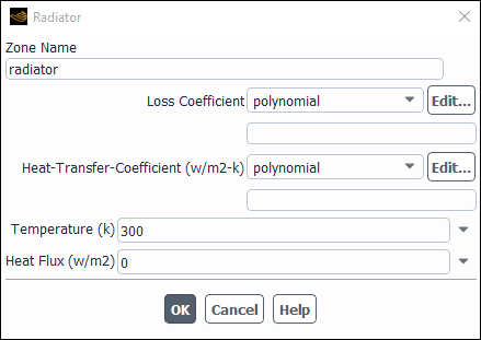
The inputs for a radiator are as follows:
Identify the radiator zone.
Define the pressure loss coefficient.
Define either the heat flux or the heat transfer coefficient and radiator temperature.
If defining the heat flux, specify the Temperature as absolute zero.
Define the discrete phase boundary condition for the radiator (for discrete phase calculations).
Since the radiator is considered to be infinitely thin, it must be modeled as the interface between cells, rather than a cell zone. Therefore the radiator zone is a type of internal face zone (where the faces are line segments in 2D or triangles/quadrilaterals in 3D). If, when you read your mesh into Ansys Fluent, the radiator zone is identified as an interior zone, right-click the zone in the tree and use the Type sub-menu to change it to a radiator zone (for more details, see Changing Cell and Boundary Zone Types).
Once the interior zone has been changed to a radiator zone, you can open the Radiator dialog box and specify the loss coefficient and heat flux information.
To define the pressure loss coefficient  you can specify a polynomial, piecewise-linear, or piecewise-polynomial function of velocity, or a constant
value.
you can specify a polynomial, piecewise-linear, or piecewise-polynomial function of velocity, or a constant
value.
Follow these steps to set a polynomial, piecewise-linear, or piecewise-polynomial function for the pressure loss coefficient:
Choose polynomial, piecewise-linear, or piecewise-polynomial in the drop-down list to the right of Loss Coefficient. (If the function type you want is already selected, you can click the button to open the dialog box where you will define the function.)
In the dialog box that appears for the definition of the Loss Coefficient function (for example, Figure 7.79: Polynomial Profile Dialog Box for Loss Coefficient Definition), enter the appropriate values. These profile input dialog boxes are used the same way as the profile input dialog boxes for temperature-dependent properties. See Defining Properties Using Temperature-Dependent Functions to find out how to use them.
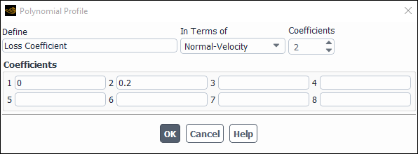
To define a constant loss coefficient, follow these steps:
Choose constant in the Loss Coefficient drop-down list.
Enter the value for
 in the Loss Coefficient field.
This example shows you how to determine the loss coefficient function. Consider the simple two-dimensional duct flow of air through a water-cooled radiator, shown in Figure 7.80: A Simple Duct with a Radiator.
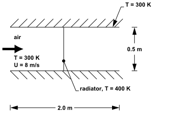
The radiator characteristics must be known empirically. For this case, assume that the radiator to be modeled yields the
test data shown in Table 7.2: Air-side Radiator Data, which was taken with a waterside flow rate of 7 kg/min and an inlet
water temperature of 400.0 K. To compute the loss coefficient, it is helpful to construct a table with values of the
dynamic head,  , as a function of pressure drop,
  , and the ratio of these two values,
  (from Equation 7–142). (The air density, defined in Figure 7.80: A Simple Duct with a Radiator, is 1.0 kg/
  .) The reduced data are shown in Table 7.3: Reduced Radiator Data.
Table 7.2: Air-side Radiator Data
| Velocity (m/s) | Upstream Temp (K) | Downstream Temp (K) | Pressure Drop |
|---|---|---|---|
| 5.0 | 300.0 | 330.0 | 75.0 |
| 10.0 | 300.0 | 322.5 | 250.0 |
| 15.0 | 300.0 | 320.0 | 450.0 |


The loss coefficient is a linear function of the velocity, decreasing as the velocity increases. The form of this relationship is
 | (7–150) |
where  is now the absolute value of the velocity through the radiator.
As mentioned in Radiator Equations, you can either define the actual heat flux  in the Heat Flux field, or set the heat transfer coefficient and radiator temperature
 . All inputs are in the Radiator Dialog Box.
To define the actual heat flux, specify a Temperature of 0 K, and set the
constant Heat Flux value.
To define the radiator temperature, enter the value for  in the Temperature field. To define the Heat-Transfer-Coefficient,
you can specify a polynomial, piecewise-linear, or piecewise-polynomial function of velocity, or a constant value.
in the Temperature field. To define the Heat-Transfer-Coefficient,
you can specify a polynomial, piecewise-linear, or piecewise-polynomial function of velocity, or a constant value.
Follow these steps to set a polynomial, piecewise-linear, or piecewise-polynomial function for the heat transfer coefficient:
Choose polynomial, piecewise-linear, or piecewise-polynomial in the drop-down list to the right of Heat-Transfer-Coefficient. (If the function type you want is already selected, you can click the button to open the dialog box where you will define the function.)
In the dialog box that appears for the definition of the Heat-Transfer-Coefficient function, enter the appropriate values. These profile input dialog boxes are used the same way as the profile input dialog boxes for temperature-dependent properties. See Defining Properties Using Temperature-Dependent Functions to find out how to use them.
To define a constant heat transfer coefficient, follow these steps:
Choose constant in the Heat-Transfer-Coefficient drop-down list.
Enter the value for
 in the Heat-Transfer-Coefficient field.
This example shows you how to determine the function for the heat transfer coefficient. Consider the simple two-dimensional duct flow of air through a water-cooled radiator, shown in Figure 7.80: A Simple Duct with a Radiator.
The data supplied in Table 7.2: Air-side Radiator Data along with values for the air density (1.0 kg/  ) and specific heat (1000 J/kg-K) can be used to obtain the following values for the heat transfer
coefficient
) and specific heat (1000 J/kg-K) can be used to obtain the following values for the heat transfer
coefficient  :
:
| Velocity (m/s) |  (W/ (W/  -K) -K)
|
|---|---|
| 5.0 | 2142.9 |
| 10.0 | 2903.2 |
| 15.0 | 3750.0 |
The heat transfer coefficient obeys a second-order polynomial relationship (fit to the points in the table above) with the velocity, which is of the form
 | (7–151) |
Note that the velocity  is assumed to be the absolute value of the velocity passing through the radiator.
If you are modeling a discrete phase of particles, you can set the fate of particle trajectories at the radiator. See Setting Boundary Conditions for the Discrete Phase for details.
You can use the Surface Integrals Dialog Box to report the pressure drop across the radiator, as described in Surface Integration. There are two steps to this procedure:
Create a surface on each side of the radiator zone. Use the Transform Surface Dialog Box (as described in Transforming Surfaces) to translate the radiator zone slightly upstream and slightly downstream to create two new surfaces.
In the Surface Integrals dialog box, report the average Static Pressure just upstream and just downstream of the radiator. You can then calculate the pressure drop across the radiator.
To check this value against the expected value based on Equation 7–142, you can use the
Surface Integrals dialog box to report the average normal velocity through the radiator. (If the radiator
is not aligned with the  ,
,  , or
, or  axis, you will need to use the Custom Field Function Calculator Dialog Box to generate a
function for the velocity normal to the radiator.) Once you have the average normal velocity, you can use Equation 7–143 to determine the loss coefficient and then Equation 7–142 to calculate
the expected pressure loss.
axis, you will need to use the Custom Field Function Calculator Dialog Box to generate a
function for the velocity normal to the radiator.) Once you have the average normal velocity, you can use Equation 7–143 to determine the loss coefficient and then Equation 7–142 to calculate
the expected pressure loss.
To determine the temperature rise across the radiator, follow the procedure outlined above for the pressure drop to generate surfaces upstream and downstream of the radiator. Then use the Surface Integrals Dialog Box (as for the pressure drop report) to report the average Static Temperature on each surface. You can then calculate the temperature rise across the radiator.
Graphical reports of interest with radiators are as follows:
Contours or profiles of Static Pressure and Static Temperature.
XY plots of Static Pressure and Static Temperature vs position.
Displaying Graphics explains how to generate graphical displays of data.
Important: When generating these plots, be sure to turn off the display of node values so that you can see the different values on each side of the radiator. (If you display node values, the cell values on either side of the radiator will be averaged to obtain a node value, and you will not see, for example, the pressure loss across the radiator.)
Porous jump conditions are used to model a thin “membrane” that has known velocity (pressure-drop) characteristics. It is essentially a 1D simplification of the porous media model available for cell zones. Examples of uses for the porous jump condition include modeling pressure drops through screens and filters, and modeling radiators when you are not concerned with heat transfer. This simpler model should be used whenever possible (instead of the full porous media model) because it is more robust and yields better convergence.
The thin porous medium has a finite thickness over which the pressure change is defined as a combination of Darcy’s Law and an additional inertial loss term:
 | (7–152) |
where  is the laminar fluid viscosity,
  is the permeability of the medium,
  is the pressure-jump coefficient,
  is the velocity normal to the porous face, and
  is the thickness of the medium. Appropriate values for
  and
and  can be calculated using the techniques described in User Inputs for Porous Media.
In a coupled analysis involving Fluent and System Coupling, data can be transferred to and from the porous jump boundary. For more about System Coupling, see Performing System Coupling Simulations Using Fluent. For more information about the data transferred, see Force transferred to System Coupling from a Porous Jump Boundary.
Note:
The porous jump boundary condition considers only the momentum resistance. Diffusion processes are not considered.
In some cases, the pressure-based coupled solver with porous jump boundary conditions may suffer from convergence issues that do not respond to changes in the coupled solver settings. This behavior depends on the specific flow configuration and porous jump boundary condition values. If convergence instability is observed using the coupled pressure-based solver, it is recommended that you change the pressure-velocity coupling to one of the segregated schemes.
Once the porous jump zone has been identified (in the Boundary Conditions task page), you will set all modeling inputs for the porous jump in the Porous Jump Dialog Box (Figure 7.81: The Porous Jump Dialog Box), which is opened from the Boundary Conditions Task Page (as described in Setting Cell Zone and Boundary Conditions ).
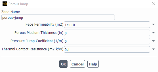
The inputs required for the porous jump model are as follows:
Identify the porous-jump zone.
Set the Face Permeability of the medium (
 in Equation 7–152).
Set the Porous Medium Thickness (
 ).
).Set the Pressure-Jump Coefficient (
 ).
). Note: The unit for the pressure-jump coefficient (C2) is the inverse of length. Should you want to define different units, you can do so by opening the Units dialog box and selecting length-inverse from the Quantities list.
Set the Thermal Contact Resistance.
Define the discrete phase boundary condition for the porous jump (for discrete phase calculations).
If you have enabled the solar load model, define the Solar Boundary Conditions for the porous jump. These settings allow you to define the boundary such that it acts as a semi-transparent surface (with respect to the solar radiation calculation only), and therefore allows a portion of the solar radiation to pass through it. See Solar Ray Tracing for details.
Since the porous jump model is a 1D simplification of the porous media model, the porous-jump zone must be modeled as the interface between cells, rather than a cell zone. Therefore the porous-jump zone is a type of internal face zone (where the faces are line segments in 2D or triangles/quadrilaterals in 3D). If the porous-jump zone is not identified as such by default when you read in the mesh (that is, if it is identified as another type of internal face zone), you can right-click the zone in the tree and use the Type sub-menu to change it to a porous-jump zone (for more details, see Changing Cell and Boundary Zone Types).
After the zone has been changed to a porous jump, you can open the Porous Jump Dialog Box (as described in Setting Cell Zone and Boundary Conditions) and specify the porous jump parameters listed above.
If you are modeling a discrete phase of particles, you can set the fate of particle trajectories at the porous jump. See Setting Boundary Conditions for the Discrete Phase for details.
Postprocessing suggestions for a problem that includes a porous jump are the same as for porous media problems. See Postprocessing for Porous Media.